T-SQL Querying (2015)
Chapter 7. Working with date and time
Working with date and time is one of the more critical topics that anyone who deals with T-SQL at any level needs to know well. That’s because almost every piece of data you store in the database has some kind of date and time element related to it. There are many pitfalls you need to be aware of that can lead to buggy and poorly performing code.
This chapter starts by covering the date and time types Microsoft SQL Server supports, followed by coverage of built-in functions that operate on the inputs of those types. It then covers challenges you face when working with date and time data and provides best practices to handle those. Finally, the chapter covers date and time querying tasks, the inefficiencies in some of the common solutions to those tasks, and creative well-performing solutions.
Date and time data types
The latest version of SQL Server at the date of this writing (SQL Server 2014) supports six date and time data types. The DATETIME and SMALLDATETIME types are longstanding features in the product. The rest of the types—DATE, TIME, DATETIME2, and DATETIMEOFFSET—are later additions that were introduced in SQL Server 2008. Table 7-1 provides the specifications of the supported date and time types.
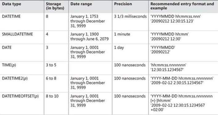
TABLE 7-1 Date and time data types
The rule of thumb in choosing a type is to use the smallest one that covers your needs in terms of date range, precision, functionality, and API support. The smaller the type is, the less storage it uses. With large tables, the saving add up, resulting in fewer reads to process queries, which in turn translates to faster queries.
The more veteran types, DATETIME and SMALLDATETIME, are still quite widely used, especially the former. That’s mainly because of legacy data, code, and habits. People usually don’t rush to alter types of columns and related code because of the complexities involved, unless there’s a compelling reason to do so. Also, when you need to store both date and time and don’t need precision finer than a minute, SMALLDATETIME is still the most economic choice.
In terms of the supported range of dates, for the types DATE, DATETIME2, and DATETIMEOFFSET, SQL Server uses the proleptic Gregorian calendar. This calendar extends support for dates that precede those that are supported by the Gregorian calendar, which was introduced in 1582. For details, see http://en.wikipedia.org/wiki/Proleptic_Gregorian_calendar.
If you do need a separation between date and time, you should use DATE and TIME, respectively. It’s more common to need to store date-only information, like order date, shipped date, invoice date, and so on. The DATE type is the most economic choice for such information. If you need to store time-only information, like business opening and closing times, the TIME type is the most economic option.
One of the trickier parts of working with the DATETIME type is its limited and awkward precision of 3 1/3 milliseconds, rounded to the nearest tick (for example, 0, 3, 7, 10, 13, 17, and so on). If this precision is not sufficient for you, you will have to use one of the other types. For example, DATETIME2 supports a level of precision of up to 100 nanoseconds. Also, the rounding treatment of this type can create problems, as I will describe later in the “Rounding issues” section.
The types TIME, DATETIME2, and DATETIMEOFFSET all support a level of precision of up to 100 nanoseconds. If you don’t need such fine precision, you can specify the level of precision in parentheses as a fraction of a second: 0 means one-second precision, and 7 (the default) means 100-nanosecond precision. Make sure you specify the lowest precision you need explicitly because this can save you up to two bytes of storage per value. For example, DATETIME(3) gives you one-millisecond precision and 7 bytes of storage instead of the maximum of 8 bytes.
As for DATETIMEOFFSET, this type is similar to DATETIME2 in that it stores the combined date and time values with up to 100-nanosecond precision. In addition, it stores the offset from UTC. This is the only type that captures the true meaning of the time when and where it was collected. With all other types, to know the true meaning of the value, you need extra information recorded such as time zone and daylight saving time state. Even though the DATETIMEOFFSET type doesn’t store the actual time zone and daylight saving time state, the value stored does take those into consideration. For example, suppose you need to store the date and time value November 1, 2015 at 1:30 AM, Pacific Daylight Time. The Pacific Time Zone (PTZ) switches from Pacific Daylight Time (PDT) to Pacific Standard Time (PST) on November 1, 2015 at 2:00 AM, setting the clock one hour backward to 1:00 AM. So, November 1, 2015, 1:30 AM, PDT is at an offset of –7 hours from UTC, which at that point is November 1, 2015, 8:30 AM. An hour later, November 1, 2015, 1:30 AM, PST is at an offset of –8 hours from UTC, which at that point is November 1, 2015, 9:30 AM. With the DATETIMEOFFSET type, you can correctly capture the two date and time values collected in PTZ as ‘20151101 01:30:00.0000000 –07:00’ and ‘20151101 01:30:00.0000000 –08:00’. You can also capture the current date and time as a DATETIMEOFFSET value using the SYSDATETIMEOFFSET function. (You’ll read more on date and time functions shortly.) Suppose you ran the following code in 2015 a few seconds before the switch from PDT to PST and a few seconds after:
SELECT SYSDATETIMEOFFSET();
I actually changed my computer clock to a few seconds before the switch and then ran the code before and after the switch. I got the following output before the switch:
----------------------------------
2015-11-01 01:59:43.8788709 -07:00
I got the following output after the switch:
----------------------------------
2015-11-01 01:00:03.4339354 -08:00
As you can see, the true meaning of the date and time values are correctly captured.
As mentioned, if you store a value in one of the other types, like DATETIME2, you need to record extra information to capture the value’s true meaning.
Some people would like to see more time zone–related capabilities in the product, like capturing the time zone name, daylight saving time state, and more.
The date and time types and functions that are supported by SQL Server do not support leap seconds. A leap second is a one-second adjustment that is occasionally applied to UTC to keep it close to mean solar time (the time as reckoned by the sun’s position in the sky). The adjustment compensates for a drift in mean solar time from atomic time as a result of irregularities in the earth’s rotation. For example, on June 30, 2012, UTC inserted a positive leap second to the last minute of the day, so the time in the last second of the day was 23:59:60, followed by midnight. In a similar way, UTC also supports the concept of a negative leap second, where the last second of the day would be 23:59:58, followed by midnight. The date and time types and functions in SQL Server ignore the concept of leap seconds. So you can neither represent a date and time value such as ‘20120630 23:59:60’, nor account for the leap seconds by using functions like DATEADD and DATEDIFF.
As for functions that return the current date and time values like SYSDATETIME, they return the values based on Microsoft Windows time, which also ignores leap seconds. The Windows Time service does receive a packet that includes a leap second from the time server, but in a sense, it ignores it. It doesn’t add or remove a second to the last minute of the day like UTC does; rather, it resolves the one-second time difference created between the local computer’s clock and the correct time in the next time synchronization. This is pretty much like correcting a time difference between the local computer’s clock and the correct time for any other reason, like for the inaccuracies of the internal computer’s clock rate. If the time difference is small, the local clock is adjusted gradually to allow it to converge toward the correct time; if the time difference is larger, it is adjusted immediately. If you need to take leap seconds into consideration in your calculations (for example, if you want to determine the difference in seconds between two UTC date and time values), you need to maintain a leap-seconds table and consult it when making your calculation.
All six supported date and time types represent a point in time. A big missing piece in SQL Server is native support for intervals of date and time in the form of a data type, related functionality, and optimization. Later in the chapter in the “Intervals” section, I will cover the current challenges in creating efficient solutions for common tasks involving date and time intervals.
Date and time functions
This section covers date and time functions supported by SQL Server. I’m going to only briefly go over the available functions and their purpose and spend more time on less trivial aspects. For full details on the functions, consult books online using the following URL:http://msdn.microsoft.com/en-us/library/ms186724(v=sql.120).aspx.
SQL Server supports six functions that return the current date and time:
SELECT
GETDATE() AS [GETDATE],
CURRENT_TIMESTAMP AS [CURRENT_TIMESTAMP],
GETUTCDATE() AS [GETUTCDATE],
SYSDATETIME() AS [SYSDATETIME],
SYSUTCDATETIME() AS [SYSUTCDATETIME],
SYSDATETIMEOFFSET() AS [SYSDATETIMEOFFSET];
GETDATE returns the current date and time of the machine on which the SQL Server instance is installed as a DATETIME value. CURRENT_TIMESTAMP (observe the lack of parentheses) is the same as GETDATE, but it is the standard version of the function. GETUTCDATE returns the current UTC date and time as a DATETIME value. SYSDATETIME and SYSUTCDATETIME are higher-precision versions of GETDATE and GETUTCDATE, respectively, returning the results as DATETIME2 values. Finally, SYSDATETIMEOFFSET returns the current date and time value including the current offset from UTC, taking daylight saving time state into consideration. As an example, in a system set to the Pacific Time Zone, during Pacific Standard Time (PST) the function will return the offset –08:00, whereas during Pacific Daylight Time (PDT) it will return the offset –07:00. Using the SYSDATETIMEOFFSET function is the best way in SQL Server to capture the true meaning of the current date and time where and when the value was collected.
There are no built-in functions returning the current date and the current time. To get those, simply cast the SYSDATETIME function’s result to the DATE and TIME types, respectively, like so:
SELECT
CAST(SYSDATETIME() AS DATE) AS [current_date],
CAST(SYSDATETIME() AS TIME) AS [current_time];
The DATEPART function extracts the specified part of the input date and time value. For example, the following code extracts the month number and the weekday number of the input date:
SELECT
DATEPART(month, '20150212') AS monthnum,
DATEPART(weekday, '20150212') AS weekdaynum;
Note that the weekday number that the function will return depends on the effective language for the connected login. For example, the input date February 12, 2015, is a Thursday. Under us_english, the function will return the weekday number 5, and under British, it will return 4. Later in the chapter in the “Identifying weekdays” section I will provide techniques to control when the week starts as part of the calculation.
The DATEPART function supports a part called TZoffset, which you use to extract the offset of an input DATETIMEOFFSET value from UTC. There’s no part you can use to extract the daylight saving time state, because this information is not stored with the value. There’s no built-in function to get the current daylight saving time state, but there are a number of ways to achieve this.
One option is to store in a table the current system’s time zone offset from UTC. For example, in a system configured with the Pacific Time Zone, you store the value –480 (for 480 minutes behind UTC) regardless of the current daylight saving time state. Then, to get the current daylight saving time state, compare the stored value with the result of the expression DATEPART(TZoffset, SYSDATETIMEOFFSET()). If they are the same, daylight saving time is off; otherwise, it’s on.
Getting the current daylight saving time state without storing time zone info in a table is trickier. You can compute this information by querying the registry, but in SQL Server this requires you to use the undocumented and unsupported extended procedure xp_regread. The registry keyBias in the hive SYSTEM\CurrentControlSet\Control\TimeZoneInformation holds the time bias for the configured time zone. It is specified as the offset in minutes UTC is from the configured time zone. For example, UTC is +480 minutes from Pacific Time, not taking daylight saving time state into consideration. Using the expression DATEPART(TZoffset, SYSDATETIMEOFFSET()), you get the active offset of the local time from UTC, taking daylight saving time states into consideration. So under PST, you get –480 and under PDT you get –420. To get the current daylight saving time state, collect the value of the Bias key into a local variable (call it @bias), and return the result of the computation SIGN(DATEPART(TZoffset, SYSDATETIMEOFFSET()) + @bias). Here’s the code required to achieve this:
DECLARE @bias AS INT;
EXEC master.dbo.xp_regread
'HKEY_LOCAL_MACHINE',
'SYSTEM\CurrentControlSet\Control\TimeZoneInformation',
'Bias',
@bias OUTPUT;
SELECT
SYSDATETIMEOFFSET() currentdatetimeoffset,
DATEPART(TZoffset, SYSDATETIMEOFFSET()) AS currenttzoffset,
SIGN(DATEPART(TZoffset, SYSDATETIMEOFFSET()) + @bias) AS currentdst;
Suppose you ran this code in a system configured with the Pacific Time Zone on May 5, 2015 at noon. Your output would look like this:
currentdatetimeoffset currenttzoffset currentdst
---------------------------------- --------------- -----------
2015-05-05 12:00:00.0000000 -07:00 -420 1
If you’re looking for a supported way to get the current daylight saving time state, you can use a CLR function. Return the result of the IsDaylightSavingTime method, applied to the property Now of the DateTime class. (DateTime.Now returns a DateTime object that is set to the current date and time on this computer.) Here’s the CLR C# code defining such a function called IsDST:
using System;
using System.Data.SqlTypes;
using Microsoft.SqlServer.Server;
public partial class TimeZone
{
[SqlFunction(IsDeterministic = false, DataAccess = DataAccessKind.None)]
public static SqlBoolean IsDST()
{
return DateTime.Now.IsDaylightSavingTime();
}
}
If you’re not familiar with developing and deploying CLR code, see Chapter 9, “Programmable objects,” for details.
Assuming you created a .dll file called C:\Temp\TimeZone\TimeZone\bin\Debug\TimeZone.dll with the assembly, use the following code to deploy it in SQL Server:
USE TSQLV3;
EXEC sys.sp_configure 'CLR Enabled', 1;
RECONFIGURE WITH OVERRIDE;
IF OBJECT_ID(N'dbo.IsDST', N'FS') IS NOT NULL DROP FUNCTION dbo.IsDST;
IF EXISTS(SELECT * FROM sys.assemblies WHERE name = N'TimeZone') DROP ASSEMBLY TimeZone;
CREATE ASSEMBLY TimeZone FROM 'C:\Temp\TimeZone\TimeZone\bin\Debug\TimeZone.dll';
GO
CREATE FUNCTION dbo.IsDST() RETURNS BIT EXTERNAL NAME TimeZone.TimeZone.IsDST;
Once the function is deployed, test it by running the following code:
SELECT
SYSDATETIMEOFFSET() currentdatetimeoffset,
DATEPART(TZoffset, SYSDATETIMEOFFSET()) AS currenttzoffset,
dbo.IsDST() AS currentdst;
Assuming you ran the code on May 5, 2015 and your system’s time zone is configured to Pacific Time, you will get the following output:
currentdatetimeoffset currenttzoffset currentdst
---------------------------------- --------------- ----------
2015-05-05 12:00:00.0000000 -07:00 -420 1
![]() Note
Note
If you manually change the time zone in the system to one with a different daylight saving time state (for example, from Pacific Time to Coordinate Universal Time), the function might not return the correct daylight saving time state because of the caching of the old value. Any of the following actions will flush the cached value: invoking the method System.Globalization.CultureInfo.CurrentCulture.ClearCachedData(), dropping and re-creating the assembly, and recycling the SQL Server service.
The functions DAY, MONTH, and YEAR are simply abbreviations of the DATEPART function for extracting the respective parts of the input value. Here’s an example for using these functions:
SELECT
DAY('20150212') AS theday,
MONTH('20150212') AS themonth,
YEAR('20150212') AS theyear;
The DATENAME function extracts the requested part name from the input value, returning it as a character string. For some parts, the function is language-dependent. For example, the expression DATENAME(month, ‘20150212’) returns February when the effective language isus_english and febbraio when it’s Italian.
The ISDATE function accepts an input character string and indicates whether it’s convertible to the DATETIME type. If for whatever reason you need to store date and time values in a character string column in a table, you can use the ISDATE function in a CHECK constraint to allow only valid values. The following example validates two input values:
SELECT
ISDATE('20150212') AS isdate20150212,
ISDATE('20150230') AS isdate20150230;
This code generates the following output showing that the first input represents a valid date and the second doesn’t:
isdate20150212 isdate20150230
-------------- --------------
1 0
You use the SWITCHOFFSET function to switch the offset of an input DATETIMEOFFSET value to a desired offset. For example, the following code returns the current date and time value in both offset –05:00 and –08:00, adjusted from the current date and time value with the system’s active offset:
SELECT
SWITCHOFFSET(SYSDATETIMEOFFSET(), '-05:00') AS [now as -05:00],
SWITCHOFFSET(SYSDATETIMEOFFSET(), '-08:00') AS [now as -08:00];
For example, if the offset of the input value is +02:00, to return the value with offset –05:00, the function will subtract seven hours from the local time.
The TODATETIMEOFFSET function helps you construct a DATETIMEOFFSET value using a local date and time value and an offset that you provide as inputs. Think of it as a helper function that saves you from messing with the conversion of the inputs to character strings, concatenating them using the right format, and then converting them to DATETIMEOFFSET. Here’s an example for using the function:
SELECT TODATETIMEOFFSET('20150212 00:00:00.0000000', '-08:00');
You can also use the function to merge information from two columns that separately hold the local date and time value and the offset into one DATETIMEOFFSET value, say, as a computed column. For example, suppose you have a table T1 with columns dt holding the local date and time value and offset holding the offset from UTC. The following code will add a computed column called dto that merges those:
ALTER TABLE dbo.T1 ADD dto AS TODATETIMEOFFSET(dt, offset);
The DATEADD function adds or subtracts a number of units of a specified part from a given date and time value. For example, the following expression adds one year to the input date:
SELECT DATEADD(year, 1, '20150212');
There’s no DATESUBTRACT function; to achieve subtraction, simply use a negative number of units.
The DATEDIFF function computes the difference between two date and time values in terms of the specified part. For example, the following expression returns the difference in terms of days between two dates:
SELECT DATEDIFF(day, '20150212', '20150213');
Note that the function ignores any parts in the inputs with a lower level of precision than the specified part. For example, consider the following expression that looks for the difference in years between the two inputs:
SELECT DATEDIFF(year, '20151231 23:59:59.9999999', '20160101 00:00:00.0000000');
The function ignores the parts of the inputs below the year and therefore concludes that the difference is 1 year, even though in practice the difference is only 100 nanoseconds.
Also note that if the inputs are DATETIMEOFFSET values, the difference is always computed in UTC terms, not in local terms, based on the stored source or target offsets. It can certainly be surprising if you’re not aware of this. For example, before you run the following code, try to answer what the result of the calculation should be:
DECLARE
@dto1 AS DATETIMEOFFSET = '20150212 10:30:00.0000000 -08:00',
@dto2 AS DATETIMEOFFSET = '20150213 22:30:00.0000000 -08:00';
SELECT DATEDIFF(day, @dto1, @dto2);
Most people would say the result should be 1, but in practice it is 2. That’s because the difference is done between the UTC values, which are 8 hours ahead of the local values. When adjusted to UTC, @dto1 doesn’t cross a date boundary, but @dto2 does.
If you want the calculation to be done differently, you first need to determine what you’re after exactly. One option is to do the calculation locally when the offsets are the same and return a NULL when they are not. This method is achieved like so:
DECLARE
@dto1 AS DATETIMEOFFSET = '20150212 10:30:00.0000000 -08:00',
@dto2 AS DATETIMEOFFSET = '20150213 22:30:00.0000000 -08:00';
SELECT
CASE
WHEN DATEPART(TZoffset, @dto1) = DATEPART(TZoffset, @dto2)
THEN DATEDIFF(day, CAST(@dto1 AS DATETIME2), CAST(@dto2 AS DATETIME2))
END;
Keep in mind, however, that under the same configured time zone, values can have different offsets at different times depending on the daylight saving time state. As mentioned earlier, during PST they will have the offset –08:00 and during PDT they will have –07:00. So another approach is to use either the source or target offset. Here’s an example using the target’s offset:
DECLARE
@dto1 AS DATETIMEOFFSET = '20150301 23:30:00.0000000 -08:00',
@dto2 AS DATETIMEOFFSET = '20150401 11:30:00.0000000 -07:00'; -- try also with -08:00
SELECT
DATEDIFF(day,
CAST(SWITCHOFFSET(@dto1, DATEPART(TZoffset, @dto2)) AS DATETIME2),
CAST(@dto2 AS DATETIME2));
One of the tricky things about working with the DATEADD and DATEDIFF functions is that they work with four-byte integers, not eight-byte ones. This means that with DATEADD you are limited in the number of units you can add, and with DATEDIFF you are limited in the number of units you can return as the difference. This limitation becomes a problem when you need to express a date and time value as an offset from a certain starting point at some level of precision, and the offset doesn’t fit in a four-byte integer. You have a similar problem when you need to apply the inverse calculation.
As an example, suppose you need to express any DATETIME2 value as an offset in multiples of 100 nanoseconds from January 1, in the year 1. The maximum offset you will need to represent is for the date and time value ‘99991231 23:59:59.9999999’, and it is the integer 3155378975999999999. Clearly, a four-byte integer isn’t sufficient here; rather, you need an eight-byte one (the BIGINT type). What would have been nice is if SQL Server supported BIGDATEADD and BIGDATEDIFF functions (or DATEADD_BIG and DATEDIFF_BIG, similar to COUNT_BIG) that worked with the BIGINT type as well as a 100-nanosecond part for such purposes. You can find and vote for such feature enhancement requests submitted to Microsoft at the following URLs: https://connect.microsoft.com/SQLServer/feedback/details/320998 and https://connect.microsoft.com/SQLServer/feedback/details/783293/.
Meanwhile, you have to resort to awkward and convoluted alternatives of your own, such as the following DATEDIFF_NS100 inline table-valued function (TVF):
USE TSQLV3;
IF OBJECT_ID(N'dbo.DATEDIFF_NS100', N'IF') IS NOT NULL
DROP FUNCTION dbo.DATEDIFF_NS100;
GO
CREATE FUNCTION dbo.DATEDIFF_NS100(@dt1 AS DATETIME2, @dt2 AS DATETIME2) RETURNS TABLE
AS
RETURN
SELECT
CAST(864000000000 AS BIGINT) * (dddiff - subdd) + ns100diff as ns100
FROM ( VALUES( CAST(@dt1 AS TIME), CAST(@dt2 AS TIME),
DATEDIFF(dd, @dt1, @dt2)
) )
AS D(t1, t2, dddiff)
CROSS APPLY ( VALUES( CASE WHEN t1 > t2 THEN 1 ELSE 0 END ) )
AS A1(subdd)
CROSS APPLY ( VALUES( CAST(864000000000 AS BIGINT) * subdd
+ (CAST(10000000 AS BIGINT) * DATEDIFF(ss, '00:00', t2) + DATEPART(ns, t2)/100)
- (CAST(10000000 AS BIGINT) * DATEDIFF(ss, '00:00', t1) + DATEPART(ns, t1)/100) ) )
AS A2(ns100diff);
GO
The function splits the calculation into differences expressed in terms of days, seconds within the day, and remaining nanoseconds—converting each difference to the corresponding multiple of 100 nanoseconds. The reason I use an inline TVF and not a scalar one is performance related. I explain this in Chapter 9 in the section “User-defined functions.”
Use the following code to test the function:
SELECT ns100
FROM dbo.DATEDIFF_NS100('20150212 00:00:00.0000001', '20160212 00:00:00.0000000');
You will get the output 315359999999999.
Sometimes you need to compute the difference not based on just one part, and rather go gradually from the less precise parts to the more precise parts. For example, suppose you want to express the difference between ‘20150212 00:00:00.0000001’ and ‘20160212 00:00:00.0000000’ as 11 months, 30 days, 23 hours, 59 minutes, 59 seconds, and 999999900 nanoseconds. You can achieve this using the following inline TVF DATEDIFFPARTS:
IF OBJECT_ID(N'dbo.DATEDIFFPARTS', N'IF') IS NOT NULL DROP FUNCTION dbo.DATEDIFFPARTS;
GO
CREATE FUNCTION dbo.DATEDIFFPARTS(@dt1 AS DATETIME2, @dt2 AS DATETIME2) RETURNS TABLE
/* The function works correctly provided that @dt2 >= @dt1 */
AS
RETURN
SELECT
yydiff - subyy AS yy,
(mmdiff - submm) % 12 AS mm,
DATEDIFF(day, DATEADD(mm, mmdiff - submm, dt1), dt2) - subdd AS dd,
nsdiff / CAST(3600000000000 AS BIGINT) % 60 AS hh,
nsdiff / CAST(60000000000 AS BIGINT) % 60 AS mi,
nsdiff / 1000000000 % 60 AS ss,
nsdiff % 1000000000 AS ns
FROM ( VALUES( @dt1, @dt2,
CAST(@dt1 AS TIME), CAST(@dt2 AS TIME),
DATEDIFF(yy, @dt1, @dt2),
DATEDIFF(mm, @dt1, @dt2),
DATEDIFF(dd, @dt1, @dt2)
) )
AS D(dt1, dt2, t1, t2, yydiff, mmdiff, dddiff)
CROSS APPLY ( VALUES( CASE WHEN DATEADD(yy, yydiff, dt1) > dt2 THEN 1 ELSE 0 END,
CASE WHEN DATEADD(mm, mmdiff, dt1) > dt2 THEN 1 ELSE 0 END,
CASE WHEN DATEADD(dd, dddiff, dt1) > dt2 THEN 1 ELSE 0 END ) )
AS A1(subyy, submm, subdd)
CROSS APPLY ( VALUES( CAST(86400000000000 AS BIGINT) * subdd
+ (CAST(1000000000 AS BIGINT) * DATEDIFF(ss, '00:00', t2) + DATEPART(ns, t2))
- (CAST(1000000000 AS BIGINT) * DATEDIFF(ss, '00:00', t1) + DATEPART(ns, t1)) ) )
AS A2(nsdiff);
GO
The function computes the year, remaining month, and remaining day differences as yy, mm, and dd, respectively. Those take into consideration a case where one unit of the part needs to be subtracted; this is required when adding the original difference in terms of that part to the source value exceeds the target value (handled in the table expression A1). The difference in terms of the remaining parts (hours, minutes, seconds, and nanoseconds) is computed based on the nanosecond difference (nsdiff) between the time portions of the source and the target (handled in the table expression A2).
Run the following code to test the function:
SELECT yy, mm, dd, hh, mi, ss, ns
FROM dbo.DATEDIFFPARTS('20150212 00:00:00.0000001', '20160212 00:00:00.0000000');
You will get the following output:
yy mm dd hh mi ss ns
--- --- --- --- --- --- ----------
0 11 30 23 59 59 999999900
Recall that earlier I mentioned that the DATEDIFF function ignores the parts in the inputs with a lower level of precision than the specified part. As an example, I explained that the expression DATEDIFF(year, ‘20151231 23:59:59.9999999’, ‘20160101 00:00:00.0000000’) returns a 1-year difference even though in practice the difference is only 100 nanoseconds. You can use the DATEDIFFPARTS function to compute a more precise difference, like so:
SELECT yy, mm, dd, hh, mi, ss, ns
FROM dbo.DATEDIFFPARTS('20151231 23:59:59.9999999', '20160101 00:00:00.0000000');
You will get the following output:
yy mm dd hh mi ss ns
--- --- --- --- --- --- ----------
0 0 0 0 0 0 100
Note that, as the comment in the function’s definition says, the function works correctly provided that @dt2 >= @dt1, assuming you have a way to enforce this using a constraint or by other means. If you can’t guarantee this and need the function to be more generic and robust, you can swap the inputs when @dt2 < @dt1 and add to the output a column called sgn with the sign of the result, like so:
IF OBJECT_ID(N'dbo.DATEDIFFPARTS', N'IF') IS NOT NULL DROP FUNCTION dbo.DATEDIFFPARTS;
GO
CREATE FUNCTION dbo.DATEDIFFPARTS(@dt1 AS DATETIME2, @dt2 AS DATETIME2) RETURNS TABLE
AS
RETURN
SELECT
sgn,
yydiff - subyy AS yy,
(mmdiff - submm) % 12 AS mm,
DATEDIFF(day, DATEADD(mm, mmdiff - submm, dt1), dt2) - subdd AS dd,
nsdiff / CAST(3600000000000 AS BIGINT) % 60 AS hh,
nsdiff / CAST(60000000000 AS BIGINT) % 60 AS mi,
nsdiff / 1000000000 % 60 AS ss,
nsdiff % 1000000000 AS ns
FROM ( VALUES( CASE WHEN @dt1 > @dt2 THEN @dt2 ELSE @dt1 END,
CASE WHEN @dt1 > @dt2 THEN @dt1 ELSE @dt2 END,
CASE WHEN @dt1 < @dt2 THEN 1
WHEN @dt1 = @dt2 THEN 0
WHEN @dt1 > @dt2 THEN -1 END ) ) AS D(dt1, dt2, sgn)
CROSS APPLY ( VALUES( CAST(dt1 AS TIME), CAST(dt2 AS TIME),
DATEDIFF(yy, dt1, dt2),
DATEDIFF(mm, dt1, dt2),
DATEDIFF(dd, dt1, dt2) ) )
AS A1(t1, t2, yydiff, mmdiff, dddiff)
CROSS APPLY ( VALUES( CASE WHEN DATEADD(yy, yydiff, dt1) > dt2 THEN 1 ELSE 0 END,
CASE WHEN DATEADD(mm, mmdiff, dt1) > dt2 THEN 1 ELSE 0 END,
CASE WHEN DATEADD(dd, dddiff, dt1) > dt2 THEN 1 ELSE 0 END ) )
AS A2(subyy, submm, subdd)
CROSS APPLY ( VALUES( CAST(86400000000000 AS BIGINT) * subdd
+ (CAST(1000000000 AS BIGINT) * DATEDIFF(ss, '00:00', t2) + DATEPART(ns, t2))
- (CAST(1000000000 AS BIGINT) * DATEDIFF(ss, '00:00', t1) + DATEPART(ns, t1)) ) )
AS A3(nsdiff);
GO
Use the following code to test the function:
SELECT sgn, yy, mm, dd, hh, mi, ss, ns
FROM dbo.DATEDIFFPARTS('20160212 00:00:00.0000000', '20150212 00:00:00.0000001');
You will get the following output:
sgn yy mm dd hh mi ss ns
---- --- --- --- --- --- --- ----------
-1 0 11 30 23 59 59 999999900
Of course, life would have been much easier had SQL Server supported an INTERVAL type like some of the other relational database management systems (RDBMSs) do. (I am holding my breath in hope of seeing such support in SQL Server in the future.)
SQL Server 2012 added support for a few more date and time functions, which I will describe next.
You get six helper functions that help you construct date and time values of the six types from their numeric components, like so:
SELECT
DATEFROMPARTS(2015, 02, 12),
DATETIME2FROMPARTS(2015, 02, 12, 13, 30, 5, 1, 7),
DATETIMEFROMPARTS(2015, 02, 12, 13, 30, 5, 997),
DATETIMEOFFSETFROMPARTS(2015, 02, 12, 13, 30, 5, 1, -8, 0, 7),
SMALLDATETIMEFROMPARTS(2015, 02, 12, 13, 30),
TIMEFROMPARTS(13, 30, 5, 1, 7);
These functions help you avoid the need to mess with constructing character-string representations of the date and time value. Without these functions, you need to worry about using the right style so that when you convert the character string to the target date and time type, it converts correctly.
The EOMONTH function returns for the given input the respective end-of-month date, typed as DATE. For example, the following code returns the last date of the current month:
SELECT EOMONTH(SYSDATETIME());
This function supports a second optional parameter you use to indicate a month offset. For example, the following code returns the last date of the previous month:
SELECT EOMONTH(SYSDATETIME(), -1);
You use the PARSE function to parse an input string as a specified target type, optionally providing a .NET culture name for the conversion. It actually uses .NET behind the scenes. This function can be used as an alternative to the CONVERT function; you can use it to provide a user-friendly culture name as opposed to the more cryptic style number used with the CONVERT function. For example, suppose you need to convert the character-string value ‘01/02/15’ to a DATE type. With CONVERT, you need to specify style 1 to get US English–based conversion (MDY) and style 3 to get British-based conversion (DMY). Using PARSE, you specify the more user-friendly culture names ‘en-US’ and ‘en-GB’, respectively, like so:
SELECT
PARSE('01/02/15' AS DATE USING 'en-US') AS [US English],
PARSE('01/02/15' AS DATE USING 'en-GB') AS [British];
However, you should be aware that while the PARSE function might be more user friendly to use than CONVERT, it’s significantly more expensive, as I will demonstrate shortly.
One of the tricky parts with all conversion functions (CAST, CONVERT, and PARSE) is that if the conversion fails, the whole query fails. There are cases where you have bad source data and you’re not certain that all inputs will successfully convert to the target type. Suppose that for inputs that don’t convert successfully you want to return a NULL as opposed to letting the entire query fail. It’s not always simple to come up with a CASE expression that applies logic that covers all potential causes for conversion failure. To address this, SQL Server provides you with TRY_ versions of the three conversion functions (TRY_CONVERT, TRY_CAST, and TRY_PARSE). These functions simply return a NULL if the conversion isn’t successful.
As an example, the following code issues two attempts to convert a character string to a DATE:
SELECT TRY_CONVERT(DATE, '20150212', 112) AS try1, TRY_CONVERT(DATE, '20150230', 112) AS try2;
The first conversion is successful, but the second one isn’t. This code doesn’t fail; rather, it returns the following output:
try1 try2
---------- ----------
2015-02-12 NULL
The TRY_ functions seem to perform similarly to their original counterparts.
You use the FORMAT function to convert an input value to a character string based on a .NET format string, optionally specifying a .NET culture name. Like PARSE, it uses .NET behind the scenes and performs badly, as I will demonstrate shortly. As an example, the following code formats the current date and time value as short date (‘d’) using US English and British cultures:
SELECT
FORMAT(SYSDATETIME(), 'd', 'en-US') AS [US English],
FORMAT(SYSDATETIME(), 'd', 'en-GB') AS [British];
Assuming you ran this code on May 8, 2015, you get the following output:
US English British
----------- -----------
5/8/2015 08/05/2015
Here’s an example for formatting the current date and time using the explicit format ‘MM/dd/yyyy’:
SELECT FORMAT(SYSDATETIME(), 'MM/dd/yyyy') AS dt;
As mentioned, the PARSE and FORMAT functions are quite inefficient, especially when compared to using more native functions, which were internally developed with a low-level language and not .NET. I’ll demonstrate this with a performance test. Run the following code to create a temporary table called #T, and fill it with 1,000,000 rows:
SELECT orderdate AS dt, CONVERT(CHAR(10), orderdate, 101) AS strdt
INTO #T
FROM PerformanceV3.dbo.Orders;
The table #T has two columns: dt holds dates as DATE-typed values, and strdt holds dates as CHAR(10)-typed values using US English format.
The first test compares the performance of PARSE with that of CONVERT to parse the values in the column strdt as DATE. To exclude the time it takes to present the values in SQL Server Management Studio (SSMS), I ran the test with results discarded (after enabling the Discard Results After Execution option under Results, Grid, in the Query Options dialog box). Here’s the code testing the PARSE function:
SELECT PARSE(strdt AS DATE USING 'en-US') AS mydt
FROM #T;
It took this code with the PARSE function over three minutes to complete on my system.
Here’s the code testing the CONVERT function to achieve the same task:
SELECT CONVERT(DATE, strdt, 101) AS mydt
FROM #T;
It took this code with the CONVERT function under a second to complete.
The second test compares FORMAT with CONVERT to format the values in dt as character strings using the format ‘MM/dd/yyyy’.
Here’s the code to achieve the task using the FORMAT function, which took 28 seconds to complete:
SELECT FORMAT(dt, 'MM/dd/yyyy') AS mystrdt
FROM #T;
Here’s the code to achieve the task using the CONVERT function, which took under a second to complete:
SELECT CONVERT(CHAR(10), dt, 101) AS mystrdt
FROM #T;
What’s interesting is that you can achieve much better performance than the supplied FORMAT function by implementing your own CLR-based date and time formatting function. You simply invoke the ToString method against the input date and time value, and provide the input format string as input to the method, as in (SqlString)dt.Value.ToString(formatstring.Value). In my test, the query with the user-defined CLR function finished in three seconds; that’s 10 times faster than with the supplied FORMAT function. In short, you better stay away from the supplied PARSE and FORMAT functions and use the suggested alternatives.
When you’re done, run the following code for cleanup:
DROP TABLE #T;
SQL Server 2014 doesn’t add support for any new date and time functions.
Challenges working with date and time
You will encounter many challenges when working with date and time data, and they are related to writing both correct and efficient code. This section covers challenges like working with literals; identifying the weekday of a date; handling date-only and time-only data; handling first, last, previous, and next date calculations; handling search arguments; and dealing with rounding issues.
Literals
Handling date and time literals is an area that tends to cause quite a lot of trouble, often leading to bugs in the code. This section describes the complexities involved with handling date and time literals and provides recommendations and best practices to help you avoid getting into trouble.
For starters, note that although standard SQL defines date and time literals, T-SQL doesn’t support those. The practice in T-SQL is to express those as character strings. Then, based on SQL Server’s implicit conversion rules, which take into consideration things like context and date type precedence, the character string gets converted to the target date and time type. For example, suppose that in the filter WHERE dt = ‘20150212’, the column dt is of a DATE type. SQL Server sees a DATE type of the column on the left side and a VARCHAR type of the literal on the right side, and its implicit conversion rules tell it to convert the literal to DATE.
The part where this conversion gets tricky is in how SQL Server interprets the value. With time literals, there’s no ambiguity, but some date literal formats are ambiguous, with their interpretation being language dependent. That is, their interpretation depends on the effective language of the login running the code (which is set as the login’s default language and can be overwritten at the session level with the SET LANGUAGE and SET DATEFORMAT options). Take the following query as an example:
USE TSQLV3;
SELECT orderid, custid, empid, orderdate
FROM Sales.Orders
WHERE orderdate = '02/12/2015';
Whether SQL Server will interpret the date as February 12, 2015 or December 2, 2015 depends on your effective language. For example, under British your session’s DATEFORMAT setting is set to dmy, and hence the value will be interpreted as December 2, 2015. You can verify this by overwriting the current session’s language using the SET LANGUAGE command, like so:
SET LANGUAGE British;
SELECT orderid, custid, empid, orderdate
FROM Sales.Orders
WHERE orderdate = '02/12/2015';
Apparently, no orders were placed on December 2, 2015, so the output is an empty set:
orderid custid empid orderdate
----------- ----------- ----------- ----------
Try the same query under US English (where DATEFORMAT is set to mdy):
SET LANGUAGE us_english;
SELECT orderid, custid, empid, orderdate
FROM Sales.Orders
WHERE orderdate = '02/12/2015';
This time, the interpretation is February 12, 2015, and the query returns the following output:
orderid custid empid orderdate
----------- ----------- ----------- ----------
10883 48 8 2015-02-12
10884 45 4 2015-02-12
10885 76 6 2015-02-12
As you can see, using an ambiguous format is a bad idea. Different logins running the same code can get different interpretations. Fortunately, a number of formats are considered language neutral, or unambiguous, such as ‘YYYYMMDD’. Try this format under both British and US English:
SET LANGUAGE British;
SELECT orderid, custid, empid, orderdate
FROM Sales.Orders
WHERE orderdate = '20150212';
SET LANGUAGE us_english;
SELECT orderid, custid, empid, orderdate
FROM Sales.Orders
WHERE orderdate = '20150212';
In both cases, you get the same interpretation of February 12, 2015.
If you insist on using a style that, in its raw form, is considered ambiguous, you can get an unambiguous interpretation by applying explicit conversion and providing information about the style you use. You can use the CONVERT function with a style number or the PARSE function with a culture name. For example, the following expressions will give you an mdy interpretation:
SELECT CONVERT(DATE, '02/12/2015', 101);
SELECT PARSE('02/12/2015' AS DATE USING 'en-US');
The following conversions will give you dmy interpretation:
SELECT CONVERT(DATE, '12/02/2015', 103);
SELECT PARSE('12/02/2015' AS DATE USING 'en-GB');
Using the CONVERT function doesn’t incur any extra cost compared to implicit conversion because conversion happens one way or the other. But keep in mind the earlier discussion about the inefficiency of the PARSE function. Using PARSE is going to cost you more.
For your convenience, Table 7-2 provides the formats that are considered unambiguous for the different date and time types.
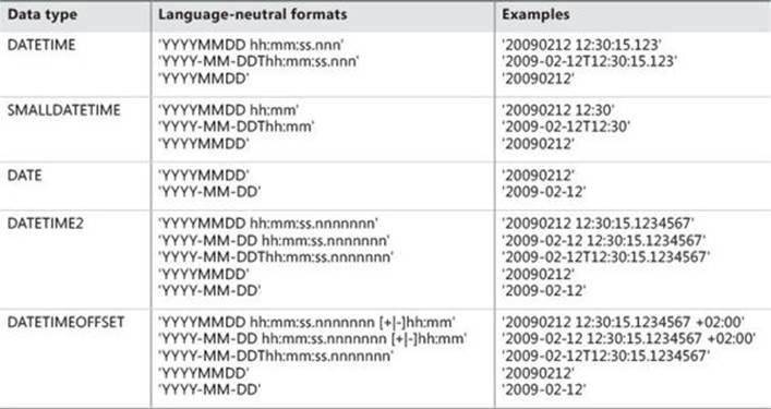
TABLE 7-2 Date and time data type formats
![]() Important
Important
The format ‘YYYY-MM-DD’ is considered unambiguous for the types DATE, DATETIME2, and DATETIMEOFFSET in accordance with the standard. However, for backward-compatibility reasons, it is considered ambiguous for the more veteran types DATETIME and SMALLDATETIME. For example, with the more veteran types, the value ‘2015-02-12’ will be interpreted as December 2, 2015 under British and February 12, 2015 under US English. With the newer types, it’s always going to be interpreted as February 12, 2015. This can lead to trouble if you’re using one of the veteran types and assuming you’ll get a British-like interpretation, and at some point alter the type of the column to one of the newer types, getting a different interpretation. For this reason, I prefer to stick to the format ‘YYYYMMDD’. It’s unambiguous across all types—with and without a time portion added. Generally, it’s recommended to stick to coding habits that give you correct and unambiguous interpretation in all cases.
Identifying weekdays
Suppose that in your application you need to identify the weekday number of an input date. You need to be aware of some complexities involved in such a calculation, and this section provides the details.
To calculate the weekday number of a given date, you can use the DATEPART function with the weekday part (or dw for short), as in DATEPART(weekday, SYSDATETIME()) for today’s weekday number. You need to be aware that this calculation is language dependent. In the previous section, I explained that your effective language determines a related session option called DATEFORMAT, which in turn determines how date literals are interpreted. In a similar way, your language determines a session option called DATEFIRST, which in turn determines what’s considered the first day of the week (1 means Monday, 2 means Tuesday, ..., 7 means Sunday). You can query the effective setting using the @@DATEFIRST function and overwrite it using the SET DATEFIRST command. However, generally changing such language settings is not recommended because there could be calculations in the session that depend on the login’s language perspective. Plus, a cached query plan created with certain language settings cannot be reused by a session with different language settings.
Suppose today is a Thursday and you are computing today’s weekday number using the expression DATEPART(weekday, SYSDATETIME()). If you are connected with US English as your language, SQL Server sets your session’s DATEFIRST setting to 7 (indicating Sunday is the first day of the week); therefore, the expression returns the weekday number 5. If you are connected with British, SQL Server sets DATEFIRST to 1 (indicating Monday is the first day of the week); therefore, the expression returns the weekday number 4. If you explicitly set DATEFIRST to, say,2 (indicating Tuesday is the first day of the week), the expression returns 3. This is illustrated in Figure 7-1, with the arrow marking the DATEFIRST setting and x being the 1-based ordinal representing the result of the expression.
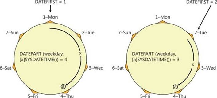
FIGURE 7-1 Language-dependent weekday.
You might run into cases where you need the weekday-number computation to assume your chosen first day of the week, ignoring the effective one. You do not want to overwrite any of the existing session’s language-related settings; rather, you want to somehow control this in the calculation itself. I can suggest a couple of methods to achieve this. I’ll refer to one method as the diff and modulo method and the other as the compensation method. For the sake of the example, suppose you want to consider Monday as the first day of the week in your calculation.
With the diff and modulo method you choose a date from the past that falls on the same weekday as the one you want to consider as the first day of the week. For this purpose, it’s convenient to use dates from the week of the base date (starting with January 1, 1900). That’s because the day parts and respective weekdays during this week are nicely aligned with the numbers and respective weekdays that DATEFIRST uses (1 for Monday, 2 for Tuesday, and so on). As an aside, curiously, for January 1, 1 was also a Monday. So, to consider Monday as the first day of the week, use the date January 1, 1900. Compute the difference in terms of days between that date and the target date (call this difference diff). The computation diff % 7 (% is modulo in T-SQL) will give you 0 for a target date whose weekday is a Monday (because diff is a multiplication of 7 in such a case), 1 for a Tuesday, and so on. Because you want to get 1 for the first day of the week, 2 for the second, and so on, simply add 1 to the computation. Here’s the complete expression in T-SQL giving you the weekday number of today’s date when considering Monday as the first day of the week:
SELECT DATEDIFF(day, '19000101', SYSDATETIME()) % 7 + 1;
To consider Sunday as the first day of the week, use the value ‘19000107’ as the starting point. If there’s some reason for you to consider Tuesday as the first day of the week, use the value ‘19000102’ as the starting point, and so on.
Another method to compute the weekday number with control over when the week starts is what I refer to as the compensation method. You use the DATEPART function with the weekday part, but instead of applying the function to the original input date, you apply it to an adjusted input date to compensate for the effect of changes in the DATEFIRST setting. Adjusting the input date by moving it @@DATEFIRST days forward neutralizes the effect of direct or indirect changes to the DATEFIRST setting.
To understand how this works, first make sure you have some coffee beside you, and then consider the following.
Let a be the original input date, and let b be the effective DATEFIRST setting (also the output of @@DATEFIRST). Let x be the original computation DATEPART(weekday, a), which is language dependent. To get a language-neutral computation, use DATEPART(weekday, DATEADD(day, b, a)). If b changes by a certain delta (such as a different language resulting in a different DATEFIRST setting), both the starting point for the calculation and the adjusted date change by the same delta, meaning that the calculation’s result remains the same. In other words, adding b (@@DATEFIRST) days to the date you’re checking compensates for any direct or indirect changes to DATEFIRST.
Now you know that regardless of the login’s language and the effective DATEFIRST setting, the computation DATEPART(weekday, DATEADD(day, @@DATEFIRST, @input)) will always return the same output for the same input. By default, the calculation behaves as if Sunday is the first day of the week. This means it will always return 1 for a Sunday, 2 for a Monday, and so on. Try it. If you want to consider a different weekday as the first day of the week, you need to further adjust the input by subtracting a constant number of days (call it c). Luckily, c and the weekday it represents are aligned with the numbers and respective weekdays DATEFIRST uses (1 for Monday, 2 for Tuesday, and so on). So, if you want to consider Monday as the first day of the week, use the expression DATEPART(weekday, DATEADD(day, @@DATEFIRST – 1, @input)). You can test the calculation with today’s date as input by using the following code:
SELECT DATEPART(weekday, DATEADD(day, @@DATEFIRST - 1, SYSDATETIME()));
The compensation method is illustrated in Figure 7-2, using today’s date as input, assuming today is a Thursday. Remember a is the input date, b is @@DATEFIRST, c is the constant you need to subtract (1 for Monday), and x is the result of the original computationDATEPART(weekday, a).
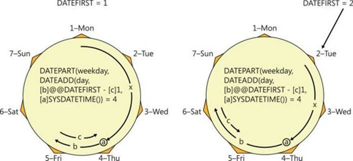
FIGURE 7-2 Language-neutral weekday.
The illustration to the left represents an environment with DATEFIRST set to 1 (where normally Monday is the first day of the week), and the illustration to the right represents an environment with DATEFIRST set to 2 (Tuesday is the first day of the week). Observe how in both cases the result is 4 assuming Monday is the first day of the week for the calculation.
Handling date-only or time-only data with DATETIME and SMALLDATETIME
As mentioned earlier, the more veteran types DATETIME and SMALLDATETIME are still quite widely used, especially the former, for historic and other reasons. The question is, how do you handle date-only and time-only data with these types, considering that they contain both elements? The recommended practice is that when you need to store the date only, you store the date with midnight as the time; and when you need to store time only, you store the time with the base date (January 1, 1900) as the date.
If you’re wondering why you specifically use midnight and the base date and not other choices, there’s a reason for this. When SQL Server converts a character string that contains the date only to a date and time type, it assumes midnight as the time. As an example, say you have a query with the filter WHERE dt = ‘20150212’, and the dt column is of a DATETIME type. SQL Server will implicitly convert the literal character string to DATETIME, assuming midnight as the time. If you stored all values in the dt column with midnight as the time, this filter will correctly return the rows where the date is February 12, 2015.
As an example for time-only data, say you have a query with the filter WHERE tm = ‘12:00:00.000’ and the tm column is of a DATETIME type. SQL Server will implicitly convert the literal character string to DATETIME, assuming the base date as the date. If you stored all values in thetm column with the base date as the date, this filter will correctly return the rows where the time is midnight.
Based on the recommended practice, you need to be able to take an input date and time value, like the SYSDATETIME function, and convert it to DATETIME or SMALLDATETIME, setting the time to midnight to capture date-only data or setting the date to the base date to capture time-only data. To capture date-only data, simply convert the input to DATE and then to DATETIME (or SMALLDATETIME), like so:
SELECT CAST(CAST(SYSDATETIME() AS DATE) AS DATETIME);
There’s a slightly more complex way to set the time part of the input to midnight, but it’s worthwhile to know it because the concept can be used in other calculations, as I will demonstrate in the next section. The method involves using a starting point that is a date from the past with midnight as the time. I like to use January 1, 1900 at midnight for this purpose. You compute the difference in terms of days between that starting point and the input value (call that difference diff). Then you add diff days to the same starting point you used to compute the difference, and you get the target date at midnight as the result. Here’s the complete calculation applied to SYSDATETIME as the input:
SELECT DATEADD(day, DATEDIFF(day, '19000101', SYSDATETIME()), '19000101');
To capture time-only data, convert the input to TIME and then to DATETIME (or SMALLDATETIME), like so:
SELECT CAST(CAST(SYSDATETIME() AS TIME) AS DATETIME);
First, last, previous, and next date calculations
This section covers calculations such as finding the date of the first or last day in a period, the date of the last or next occurrence of a certain weekday, and so on. All calculations that I’ll cover are with respect to some given date and time value. I’ll use the SYSDATETIME function as the given value, but you can change SYSDATETIME to any date and time value.
First or last day of a period
This section covers calculations of the first and last date in a period, such as the month or year, with respect to some given reference date and time value.
Earlier I provided the following expression to set the time part of a given date and time value to midnight:
SELECT DATEADD(day, DATEDIFF(day, '19000101', SYSDATETIME()), '19000101');
You can use similar logic to calculate the date of the first day of the month. You need to make sure you use an anchor date that is a first day of a month and use the month part instead of the day part, like so:
SELECT DATEADD(month, DATEDIFF(month, '19000101', SYSDATETIME()), '19000101');
This expression calculates the difference in terms of whole months between some first day of a month and the reference date. Call that difference diff. The expression then adds diff months to the anchor date, producing the date of the first day of the month corresponding to the given reference date.
An alternative method to compute the first day of the month is to use the DATEFROMPARTS function, like so:
SELECT DATEFROMPARTS(YEAR(SYSDATETIME()), MONTH(SYSDATETIME()), 1);
To return the date of the last day of the month, you can use the previous calculation I showed for beginning of month, but with an anchor date that is an end of a month, like so:
SELECT DATEADD(month, DATEDIFF(month, '18991231', SYSDATETIME()), '18991231');
Note that it’s important to use an anchor date that is a 31st of some month, such as December, so that if the target month has 31 days the calculation works correctly.
Specifically with the end of month calculation, you don’t need to work that hard because T-SQL supports the EOMONTH function described earlier:
SELECT EOMONTH(SYSDATETIME());
To calculate the date of the first day of the year, use an anchor that is a first day of some year, and specify the year part, like so:
SELECT DATEADD(year, DATEDIFF(year, '19000101', SYSDATETIME()), '19000101');
Or you could use the DATEFROMPARTS function, like so:
SELECT DATEFROMPARTS(YEAR(SYSDATETIME()), 1, 1);
To calculate the date of the last day of the year, use an anchor date that is the last day of some year:
SELECT DATEADD(year, DATEDIFF(year, '18991231', SYSDATETIME()), '18991231');
Or, again, you could use the DATEFROMPARTS function, like so:
SELECT DATEFROMPARTS(YEAR(SYSDATETIME()), 12, 31);
Previous or next weekday
This section covers calculations that return a next or previous weekday with respect to a given date and time value. I use the word respective to describe this sort of calculation.
Suppose you need to calculate the latest Monday before or on a given reference date and time. The calculation needs to be inclusive of the reference date. That is, if the reference date is a Monday, return the reference date; otherwise, return the latest Monday before the reference date. You can use the following expression to achieve this:
SELECT DATEADD(
day,
DATEDIFF(
day,
'19000101', -- Base Monday date
SYSDATETIME()) /7*7,
'19000101'); -- Base Monday date
The expression calculates the difference in terms of days between some anchor date that is a Monday and the reference date. Call that difference diff.
As I mentioned earlier, it’s convenient to use dates in the range January 1, 1900, and January 7, 1900, as anchor dates because they represent the weekdays Monday through Sunday, respectively. The day parts of the suggested anchor dates (1 through 7) are aligned with the integers used in SQL Server to represent the first day of the week; therefore, it’s easy to remember which day of the week each date in the range represents.
The expression then rounds the value down to the nearest multiple of 7 by dividing diff by 7 using integer division, and then multiplying it by 7. Call the result floor_diff. Note that the calculation of floor_diff will work correctly only when the result of DATEDIFF is nonnegative. So make sure you use an anchor date that is earlier than the reference date. The expression then adds floor_diff days to the anchor date, producing the latest occurrence of a Monday, inclusive. Remember that by inclusive I mean that if the reference date is a Monday, the calculation is supposed to return the reference date.
Here’s the expression formatted in one line of code:
SELECT DATEADD(day, DATEDIFF(day, '19000101', SYSDATETIME()) /7*7, '19000101');
Similarly, to return the date of the last Tuesday, use an anchor date that is a Tuesday:
SELECT DATEADD(day, DATEDIFF(day, '19000102', SYSDATETIME()) /7*7, '19000102');
And to return the date of the last Sunday, use an anchor date that is a Sunday:
SELECT DATEADD(day, DATEDIFF(day, '19000107', SYSDATETIME()) /7*7, '19000107');
To make the calculation exclusive of the reference date—meaning that you’re after the last occurrence of a weekday before the reference date (as opposed to on or before)—simply subtract a day from the reference date. For example, the following expression returns the date of the last occurrence of a Monday before the reference date:
SELECT DATEADD(day, DATEDIFF(day, '19000101', DATEADD(day, -1, SYSDATETIME())) /7*7,
'19000101');
To return the next occurrence of a weekday in an inclusive manner (on or after the reference date), subtract a day from the reference date and add 7 days to floor_diff. For example, the following expression returns the next occurrence of a Monday on or after the reference date:
SELECT DATEADD(day, DATEDIFF(day, '19000101', DATEADD(day, -1, SYSDATETIME())) /7*7 + 7,
'19000101');
Like before, replace the anchor date if you need to handle a different weekday—for example, Tuesday:
SELECT DATEADD(day, DATEDIFF(day, '19000102', DATEADD(day, -1, SYSDATETIME())) /7*7 + 7,
'19000102');
Or Sunday:
SELECT DATEADD(day, DATEDIFF(day, '19000107', DATEADD(day, -1, SYSDATETIME())) /7*7 + 7,
'19000107');
To make the calculation exclusive, meaning the next occurrence of a weekday after the reference date (as opposed to on or after), simply skip the step of subtracting a day from the anchor date. For example, the following expression returns the next occurrence of a Monday after the reference date:
SELECT DATEADD(day, DATEDIFF(day, '19000101', SYSDATETIME()) /7*7 + 7, '19000101');
This calculation is for the next occurrence of a Tuesday, exclusive:
SELECT DATEADD(day, DATEDIFF(day, '19000102', SYSDATETIME()) /7*7 + 7, '19000102');
This calculation is for the next occurrence of a Sunday, exclusive:
SELECT DATEADD(day, DATEDIFF(day, '19000107', SYSDATETIME()) /7*7 + 7, '19000107');
First or last weekday
In this section, I’ll describe calculations that return the first and last occurrences of a certain weekday in a period such as a month or year. To calculate the first occurrence of a certain weekday in a month, you need to combine two types of calculations I described earlier. One is the calculation of the first day of the month:
SELECT DATEADD(month, DATEDIFF(month, '19000101', SYSDATETIME()), '19000101');
The other is the calculation of the next occurrence of a weekday, inclusive—Monday, in this example:
SELECT DATEADD(day, DATEDIFF(day, '19000101', DATEADD(day, -1, SYSDATETIME())) /7*7 + 7,
'19000101');
The trick is to simply use the first day of the month calculation as the reference date within the next-weekday-occurrence calculation. For example, the following expression returns the first occurrence of a Monday in the reference month:
SELECT DATEADD(day, DATEDIFF(day, '19000101',
-- first day of month
DATEADD(month, DATEDIFF(month, '19000101', SYSDATETIME()), '19000101')
-1) /7*7 + 7, '19000101');
To handle a different weekday, replace the anchor date in the part of the expression that calculates the next occurrence of a weekday—not in the part that calculates the first month day. The following expression returns the date of the first occurrence of a Tuesday in the reference month:
SELECT DATEADD(day, DATEDIFF(day, '19000102',
-- first day of month
DATEADD(month, DATEDIFF(month, '19000101', SYSDATETIME()), '19000101')
-1) /7*7 + 7, '19000102');
To calculate the date of the last occurrence of a weekday in the reference month, you need to combine two calculations as well. One is the calculation of the last day of the reference month:
SELECT DATEADD(month, DATEDIFF(month, '18991231', SYSDATETIME()), '18991231');
The other is the calculation of the previous occurrence of a weekday, inclusive—Monday, in this example:
SELECT DATEADD(day, DATEDIFF(day, '19000101', SYSDATETIME()) /7*7, '19000101');
Simply use the last day of the month calculation as the reference date in the last-weekday calculation. For example, the following expression returns the last occurrence of a Monday in the reference month:
SELECT DATEADD(day, DATEDIFF(day, '19000101',
-- last day of month
DATEADD(month, DATEDIFF(month, '18991231', SYSDATETIME()), '18991231')
) /7*7, '19000101');
To address a different weekday, substitute the anchor date in the last weekday calculation with the applicable one. For example, the following expression returns the last occurrence of a Tuesday in the reference month:
SELECT DATEADD(day, DATEDIFF(day, '19000102',
-- last day of month
DATEADD(month, DATEDIFF(month, '18991231', SYSDATETIME()), '18991231')
) /7*7, '19000102');
In a manner similar to calculating the first and last occurrences of a weekday in the reference month, you can calculate the first and last occurrence of a weekday in the reference year. Simply substitute the first-month-day or last-month-day calculation with the first-year-day or last-year-day calculation. Following are a few examples.
The first occurrence of a Monday in the reference year:
SELECT DATEADD(day, DATEDIFF(day, '19000101',
-- first day of year
DATEADD(year, DATEDIFF(year, '19000101', SYSDATETIME()), '19000101')
-1) /7*7 + 7, '19000101');
The first occurrence of a Tuesday in the reference year:
SELECT DATEADD(day, DATEDIFF(day, '19000102',
-- first day of year
DATEADD(year, DATEDIFF(year, '19000101', SYSDATETIME()), '19000101')
-1) /7*7 + 7, '19000102');
The last occurrence of a Monday in the reference year:
SELECT DATEADD(day, DATEDIFF(day, '19000101',
-- last day of year
DATEADD(year, DATEDIFF(year, '18991231', SYSDATETIME()), '18991231')
) /7*7, '19000101');
The last occurrence of a Tuesday in the reference year:
SELECT DATEADD(day, DATEDIFF(day, '19000102',
-- last day of year
DATEADD(year, DATEDIFF(year, '18991231', SYSDATETIME()), '18991231')
) /7*7, '19000102');
Search argument
One of the most fundamental concepts in query tuning is that of a search argument (SARG). It’s not really unique to working with date and time data, but it is very common with such data. Suppose that you have a query with a filter in the form WHERE <column> <operator> <value> and a supporting index on the filtered column. As long as you don’t apply manipulation to the filtered column, SQL Server can rely on the index order—for example, to consider performing a seek followed by a range scan in the index. If the index is not a covering one, of course there would be the question of whether the selectivity of the filter is high enough to justify using the index, but the point is that the potential is there. If you do apply manipulation to the column, besides some exceptional cases, this might result in SQL Server not relying on the index order and using less optimal access methods like full scans.
As mentioned, the issue of SARGablility is not really unique to date and time data but is quite common in that scenario, because you often filter data based on date and time. A classic example is filtering range-of-date and time values like a whole day, week, month, quarter, year, and so on. To allow optimal index usage, you should get into the habit of expressing the range filter without manipulating the filtered column. As an example, the following two queries are logically equivalent—both filtering the entire order year 2014:
USE PerformanceV3;
SELECT orderid, orderdate, filler
FROM dbo.Orders
WHERE YEAR(orderdate) = 2014;
SELECT orderid, orderdate, filler
FROM dbo.Orders
WHERE orderdate >= '20140101'
AND orderdate < '20150101';
There’s a clustered index defined on the orderdate column, so clearly the optimal plan here is to perform a seek followed by a range scan of the qualifying rows in the index. Figure 7-3 shows the actual plans you do get for these queries.
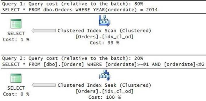
FIGURE 7-3 Non-SARG versus SARG.
The predicate in the first query is non SARGable. The optimizer doesn’t try to be smart and understand the meaning of what you’re doing; rather, it just resorts to a full scan. With the second query, the predicate is SARGable, allowing an efficient seek and partial scan in the index.
As mentioned, there are exceptions where SQL Server will consider a predicate that applies manipulation to the filtered column as SARGable. An example for such an exception is when the predicate converts the column to the DATE type, as in the following query:
SELECT orderid, orderdate, filler
FROM dbo.Orders
WHERE CAST(orderdate AS DATE) = '20140212';
Microsoft added logic to the optimizer to consider such a predicate as SARGable, and hence it chooses here to perform a seek and a range scan in the index. The problem is, this example is the exception and not the norm.
If you’re an experienced database practitioner, it’s likely that other people mimic your coding practices without always fully understanding them. For this reason, as a general rule, you should prefer the form without manipulation whenever possible because that’s the one that is more likely to be SARGable. So instead of using the predicate form in the preceding query, it’s recommended to use the following form:
SELECT orderid, orderdate, filler
FROM dbo.Orders
WHERE orderdate >= '20140212'
AND orderdate < '20140213';
Rounding issues
When you convert a character-string value to a date and time type, or convert one from a higher level of precision to a lower one, you need to be aware of how SQL Server handles such conversions. Some find SQL Server’s treatment surprising.
One of the common pitfalls occurs when converting a character-string value to the DATETIME type. To demonstrate this, I’ll use the following sample data:
USE TSQLV3;
IF OBJECT_ID(N'Sales.MyOrders', N'U') IS NOT NULL DROP TABLE Sales.MyOrders;
GO
SELECT * INTO Sales.MyOrders FROM Sales.Orders;
ALTER TABLE Sales.MyOrders ALTER COLUMN orderdate DATETIME NOT NULL;
CREATE CLUSTERED INDEX idx_cl_od ON Sales.MyOrders(orderdate);
Suppose you need to filter the orders where the order date falls within a certain date and time range. Imagine that the time part in the stored values wasn’t necessarily midnight and you want to filter a range like a whole day, month, year, and so on. For example, filter only the orders placed on January 1, 2015. A common yet incorrect way for people to express the filter is using the BETWEEN predicate, like so:
SELECT orderid, orderdate, custid, empid
FROM Sales.MyOrders
WHERE orderdate BETWEEN '20150101' AND '20150101 23:59:59.999';
When using this form, people think that 999 is the last expressible millisecond part of the second. However, recall that the precision of the DATETIME type is 3 1/3 milliseconds, rounded to the nearest tick. So the only valid values for the last digit of the milliseconds part are 0, 3, and 7. Any other value gets rounded to the closest supported one. This means that the value specified as the end delimiter in the preceding query is rounded up to midnight in the next day. This causes the query to return the following output:
orderid orderdate custid empid
----------- ----------------------- ----------- -----------
10808 2015-01-01 00:00:00.000 55 2
10809 2015-01-01 00:00:00.000 88 7
10810 2015-01-01 00:00:00.000 42 2
10811 2015-01-02 00:00:00.000 47 8
10812 2015-01-02 00:00:00.000 66 5
Observe that even though you were looking for only orders placed on January 1, 2015, you’re also getting the ones from the 2nd. For this reason, the recommended practice is to express your range as greater than or equal to midnight of the first date in the range and less than midnight of the date immediately following the last date in the range. In our example, you should change your filter like so:
SELECT orderid, orderdate, custid, empid
FROM Sales.MyOrders
WHERE orderdate >= '20150101'
AND orderdate < '20150102';
And this time you get the correct result:
orderid orderdate custid empid
----------- ---------- ----------- -----------
10808 2015-01-01 55 2
10809 2015-01-01 88 7
10810 2015-01-01 42 2
If you follow this practice, your code will work correctly with all date and time types, whether the values include a relevant time portion or not. It’s always good to get used to forms that work correctly in all cases.
Back to our example with the DATETIME column, to return orders placed today manipulate the result of the SYSDATETIME function to compute today at midnight and tomorrow at midnight as the delimiters of the closed-open interval, like so:
SELECT orderid, orderdate, custid, empid
FROM Sales.MyOrders
WHERE orderdate >= CAST(CAST(SYSDATETIME() AS DATE) AS DATETIME)
AND orderdate < DATEADD(day, 1, CAST(CAST(SYSDATETIME() AS DATE) AS DATETIME));
When you’re done, run the following code for cleanup:
IF OBJECT_ID(N'Sales.MyOrders', N'U') IS NOT NULL DROP TABLE Sales.MyOrders;
You might not be aware that SQL Server applies similar rounding logic also when converting from a higher precision date and time value to a lower precision one. For example, when you convert the result of the SYSDATETIME function (returns a DATETIME2 value) to SMALLDATETIME (minute precision), SQL Server doesn’t floor the value to the bottom of the minute; rather, it rounds the value to the closest minute. This means the value is rounded to the beginning of the minute before the half-minute point and to the next minute on or beyond that point. If you want to apply flooring instead of rounding logic, subtract 30 seconds before converting the value. The following code returns the result of the SYSDATETIME function, demonstrating both the rounding and flooring of the value:
SELECT
SYSDATETIME() AS currentdatetime,
CAST(SYSDATETIME() AS SMALLDATETIME) AS roundedtominute,
CAST(DATEADD(ss, -30, SYSDATETIME()) AS SMALLDATETIME) AS flooredtominute;
Suppose you ran this code when SYSDATETIME returns ‘2015-02-12 13:47:53.7996475’. You will get the following output:
currentdatetime roundedtominute flooredtominute
--------------------------- ----------------------- -----------------------
2015-02-12 13:47:53.7996475 2015-02-12 13:48:00 2015-02-12 13:47:00
The same rounding logic applies with any conversion from a higher precision date and time value to a lower one. For example, convert the result of SYSDATETIME to DATETIME(0), and you get rounding to the closest second. If you want to floor the value to the beginning of the second, subtract 500 milliseconds before converting. Here’s the code demonstrating both rounding and flooring with a granularity of a second:
SELECT
SYSDATETIME() AS currentdatetime,
CAST(SYSDATETIME() AS DATETIME2(0)) AS roundedtosecond,
CAST(DATEADD(ms, -500, SYSDATETIME()) AS DATETIME2(0)) AS flooredtosecond;
Again, assume you ran this code when SYSDATETIME returns ‘2015-02-12 13:47:53.7996475’. You will get the following output:
currentdatetime roundedtosecond flooredtosecond
--------------------------- --------------------------- ---------------------------
2015-02-12 13:47:53.7996475 2015-02-12 13:47:54 2015-02-12 13:47:53
Querying date and time data
This section covers the handling of querying tasks involving date and time data. It starts by providing a method to group data by week, and then provides solutions to various querying tasks involving date and time intervals.
Grouping by the week
Suppose you need to query the Sales.OrderValues view, group the rows by the order week (based on the order date), and return for each group the count of orders and total order values. As it turns out, the task is not as trivial as it might have seemed at the beginning. The main challenge is to compute a common week identifier for all dates that are associated with the same week. If you’re thinking of the DATEPART function with the week part (or wk or ww for short), this part gives you the week number in the year. If a week starts in one year and ends in another, the first few days will give you a different week number than the last few days. You need a different solution.
The solution I like to use is to compute for each date the respective start-of-week date, and then use that as my week identifier. The first step in the calculation is to compute the weekday number of the input date (call it wd). This is done using the DATEPART function with the weekday part: DATEPART(weekday, orderdate). Remember that this calculation is language dependent; it reflects the effective DATEFIRST setting based on the language of the login running the code. If you want the login’s perspective to determine when the week starts, you have your final wdvalue and therefore you’re done with the first step. If you need the calculation itself to control where the week starts, you have two different methods to achieve this as I explained earlier—the diff and modulo method, and the compensation method. For example, using the compensation method and considering Monday as the first day of the week, use the expression DATEPART(weekday, DATEADD(day, @@DATEFIRST –1, orderdate)).
Now that you have wd, the second step is to compute the distance of the input date from the respective start-of-week date (call it dist). Fortunately, that’s a simple calculation: a date with wd = N is at a distance of N – 1 days from the respective start-of-week date. For example, a date withwd = 3 is 2 days away from the respective start-of-week date. So the expression to compute dist is wd – 1.
The third and last step is to compute the respective start-of-week date (call it startofweek). That’s done by subtracting dist days from orderdate using the following expression: DATEADD(day, –dist, orderdate). You now have your week identifier and can use it as the only element in the grouping set of your grouped query.
Here’s the complete solution code:
USE TSQLV3;
SELECT
startofweek,
DATEADD(day, 6, startofweek) AS endofweek,
SUM(val) AS totalval,
COUNT(*) AS numorders
FROM Sales.OrderValues
CROSS APPLY ( VALUES( DATEPART(weekday, DATEADD(day, @@DATEFIRST -1, orderdate)) ) ) AS A1(wd)
CROSS APPLY ( VALUES( wd - 1 ) ) AS A2(dist)
CROSS APPLY ( VALUES( DATEADD(day, -dist, orderdate) ) ) AS A3(startofweek)
GROUP BY startofweek;
Observe that to also return the end-of-week date (call it endofweek), you simply add six days to startofweek. This query generates the following output:
startofweek endofweek totalval numorders
----------- ---------- --------- -----------
2013-07-01 2013-07-07 2303.40 2
2013-07-08 2013-07-14 10296.48 6
2013-07-15 2013-07-21 5306.03 6
2013-07-22 2013-07-28 4675.99 5
2013-07-29 2013-08-04 8160.00 6
...
2015-04-06 2015-04-12 21074.05 17
2015-04-13 2015-04-19 52976.83 17
2015-04-20 2015-04-26 15460.63 16
2015-04-27 2015-05-03 21720.42 17
2015-05-04 2015-05-10 12885.07 11
Intervals
An interval in mathematics is the set of values between some lower and upper values. A date and time interval is, therefore, the set of date and time values between some lower and upper values, with the granularity being based on the data type’s precision. The need to store and manipulate date and time intervals in databases is quite common. They represent things like sessions, chats, phone calls, validity periods, appointments, contracts, projects, patients’ visits to hospitals, and so on.
Common querying tasks related to intervals include identifying intervals that intersect with an input one, computing the maximum number of concurrent intervals, packing intervals, and others. Creating correct solutions for such tasks is not all that difficult. There are fairly simple classic solutions. But as it turns out, creating solutions that are both correct and perform well is far from being trivial. Achieving good performance is tricky mainly because of the fundamental optimization challenges I described in Chapter 2, “Query tuning,” concerning filters with multiple range predicates. Here you will see practical examples where this problem manifests itself. Fortunately, there are efficient solutions, although they are not as simple as the classic ones.
To demonstrate how to solve common tasks involving date and time intervals, I will use sample data representing mobile phone accounts and phone call sessions. Run the following code to create and populate the Accounts and Sessions tables in tempdb with a small set of sample data:
SET NOCOUNT ON;
USE tempdb;
IF OBJECT_ID('dbo.Sessions') IS NOT NULL DROP TABLE dbo.Sessions;
IF OBJECT_ID('dbo.Accounts') IS NOT NULL DROP TABLE dbo.Accounts;
CREATE TABLE dbo.Accounts
(
actid INT NOT NULL,
CONSTRAINT PK_Accounts PRIMARY KEY(actid)
);
GO
INSERT INTO dbo.Accounts(actid) VALUES(1), (2), (3);
CREATE TABLE dbo.Sessions
(
sessionid INT NOT NULL IDENTITY(1, 1),
actid INT NOT NULL,
starttime DATETIME2(0) NOT NULL,
endtime DATETIME2(0) NOT NULL,
CONSTRAINT PK_Sessions PRIMARY KEY(sessionid),
CONSTRAINT CHK_endtime_gteq_starttime
CHECK (endtime >= starttime)
);
GO
INSERT INTO dbo.Sessions(actid, starttime, endtime) VALUES
(1, '20151231 08:00:00', '20151231 08:30:00'),
(1, '20151231 08:30:00', '20151231 09:00:00'),
(1, '20151231 09:00:00', '20151231 09:30:00'),
(1, '20151231 10:00:00', '20151231 11:00:00'),
(1, '20151231 10:30:00', '20151231 12:00:00'),
(1, '20151231 11:30:00', '20151231 12:30:00'),
(2, '20151231 08:00:00', '20151231 10:30:00'),
(2, '20151231 08:30:00', '20151231 10:00:00'),
(2, '20151231 09:00:00', '20151231 09:30:00'),
(2, '20151231 11:00:00', '20151231 11:30:00'),
(2, '20151231 11:32:00', '20151231 12:00:00'),
(2, '20151231 12:04:00', '20151231 12:30:00'),
(3, '20151231 08:00:00', '20151231 09:00:00'),
(3, '20151231 08:00:00', '20151231 08:30:00'),
(3, '20151231 08:30:00', '20151231 09:00:00'),
(3, '20151231 09:30:00', '20151231 09:30:00');
A phone call session is an interval defined by the delimiters starttime and endtime with a granularity of a second using the type DATETIME2(0). I will leave the aspect of whether each of the delimiters is an open (exclusive) or closed (inclusive) one undefined so that you can define it on a case-by-case basis, depending on what real-life scenario you need the sample data to represent for you.
Use the small set of sample data created by the preceding code to verify the correctness of the solutions. For performance testing, you can use the following code, which creates a large set of sample data with 50 accounts and 10,000,000 intervals:
-- 10,000,000 intervals
DECLARE
@num_accounts AS INT = 50,
@sessions_per_account AS INT = 200000,
@start_period AS DATETIME2(3) = '20120101',
@end_period AS DATETIME2(3) = '20160101',
@max_duration_in_seconds AS INT = 3600; -- 1 hour
TRUNCATE TABLE dbo.Sessions;
TRUNCATE TABLE dbo.Accounts;
INSERT INTO dbo.Accounts(actid)
SELECT A.n AS actid
FROM TSQLV3.dbo.GetNums(1, @num_accounts) AS A;
WITH C AS
(
SELECT A.n AS actid,
DATEADD(second,
ABS(CHECKSUM(NEWID())) %
(DATEDIFF(s, @start_period, @end_period) - @max_duration_in_seconds),
@start_period) AS starttime
FROM TSQLV3.dbo.GetNums(1, @num_accounts) AS A
CROSS JOIN TSQLV3.dbo.GetNums(1, @sessions_per_account) AS I
)
INSERT INTO dbo.Sessions WITH (TABLOCK) (actid, starttime, endtime)
SELECT actid, starttime,
DATEADD(second,
ABS(CHECKSUM(NEWID())) % (@max_duration_in_seconds + 1),
starttime) AS endtime
FROM C;
Feel free to change the parameters for the sample data if you want to test the solutions with different data characteristics.
Intersection
An interval intersection test checks whether two intervals have any form of intersection. James F. Allen defines 13 relations between intervals, which are known as Allen’s interval algebra. (For details, see http://www.ics.uci.edu/~alspaugh/cls/shr/allen.html.) Out of the 13, 11 relations represent different forms of intersection. Those are all of Allen’s relations except before and after.
As an example, suppose you get as inputs an account id (@actid) and a closed interval [@s, @e] (with @s for start and @e for end), and your task is to return all account intervals from the Sessions table that intersect with the input one. The classic way in SQL to identify intersection is actually quite straightforward, using the predicates starttime <= @e AND endtime >= @s. These two range predicates are specified in addition to the equality predicate actid = @actid. The problem is that this classic method is often very inefficient in T-SQL. Recall the discussion about multiple range predicates in Chapter 2. Whether you create an index on the key list (actid, starttime, endtime) or (actid, endtime, starttime), only one range predicate can be used as a seek predicate (in addition to any equality predicates against leading keys). All rows that satisfy the seek predicates are scanned, and then the remaining range predicates are applied to the scanned rows as residual predicates.
You could be lucky if most queries target a limited period at the edge of the entire period covered by your data, constituting a small percentage of it. For example, usually for billing purposes you need to look for intervals that intersect only with a very recent period (last month/week). But then it’s very easy to fall into a trap from an indexing standpoint. The intuitive key order for most people to define in the index is (starttime, endtime); that’s following the equality column actid, of course. Remember that when you have multiple range predicates in your filter, you want the more selective one to appear first so that the range scan in the index leaf needs to scan a smaller range. Now think about it; which of the predicates is more selective when querying a recent period: starttime <= @e or endtime >= @s? Clearly, it’s the latter. But with an index on (starttime,endtime), your leading range key is the far less selective one, so the range scan will end up scanning most rows for the account in question.
To demonstrate this, first create the intuitive but less efficient index by running the following code:
CREATE UNIQUE INDEX idx_start_end ON dbo.Sessions(actid, starttime, endtime, sessionid);
Suppose you need to look for active sessions for account ID 1, during the hour between 11:00 AM and noon in the last day recorded (December 31, 2015). You issue the following query (RECOMPILE is used to apply parameter embedding):
DECLARE
@actid AS INT = 1,
@s AS DATETIME2(0) = '20151231 11:00:00',
@e AS DATETIME2(0) = '20151231 12:00:00';
SELECT sessionid, actid, starttime, endtime
FROM dbo.Sessions
WHERE actid = @actid
AND starttime <= @e
AND endtime >= @s
OPTION(RECOMPILE);
Here’s the output you get with the small set of sample data just to verify the validity of the code:
sessionid actid starttime endtime
---------- ------ -------------------- --------------------
4 1 2015-12-31 10:00:00 2015-12-31 11:00:00
5 1 2015-12-31 10:30:00 2015-12-31 12:00:00
6 1 2015-12-31 11:30:00 2015-12-31 12:30:00
Figure 7-4 illustrates how much data needs to be scanned in the leaf of the intuitive yet less efficient index (to the left) versus the less intuitive but more efficient one (to the right).
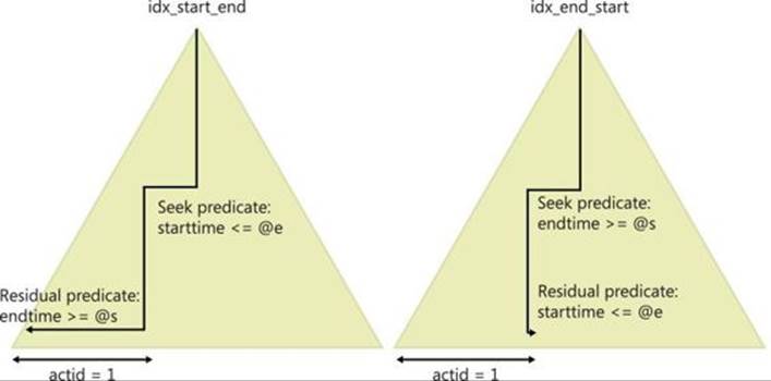
FIGURE 7-4 Indexing strategies for interval intersection queries.
The figure shows which range predicate is applied as a seek predicate for determining how many rows need to be scanned in the index leaf, and which predicate is applied as a residual predicate and evaluated against all remaining rows. As you can see, with an index on (starttime,endtime) most rows for account ID 1 need to be scanned, whereas with an index on (endtime, starttime) only a small percentage needs to be scanned.
Figure 7-5 shows the actual plan I got for the query against the large set of sample data.
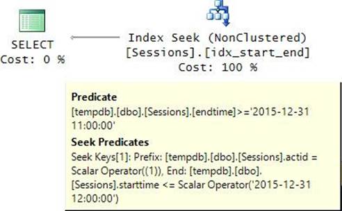
FIGURE 7-5 Interval intersection with index idx_start_end.
Observe that the less selective predicate starttime <= ‘2015-12-31 12:00:00’ appears as a seek predicate and the more selective one endtime >= ‘2015-12-31 11:00:00’ appears as a residual predicate. I populated the table with 200,000 rows per account, and with about 300 rows fitting in a page, you get about 650 pages used per account. With the current index idx_start_end, most of those pages need to be scanned. When I ran this intersection query against the large set of sample data, it performed 648 logical reads.
The conclusion is that you’re better off creating the index with the more selective column endtime appearing before the less selective column starttime, like so:
CREATE UNIQUE INDEX idx_end_start ON dbo.Sessions(actid, endtime, starttime, sessionid);
Rerun the query:
DECLARE
@actid AS INT = 1,
@s AS DATETIME2(0) = '20151231 11:00:00',
@e AS DATETIME2(0) = '20151231 12:00:00';
SELECT sessionid, actid, starttime, endtime
FROM dbo.Sessions
WHERE actid = @actid
AND starttime <= @e
AND endtime >= @s
OPTION(RECOMPILE);
This time, you get the plan in Figure 7-6, showing the more selective column used as a seek predicate and the less selective one used as a residual predicate.
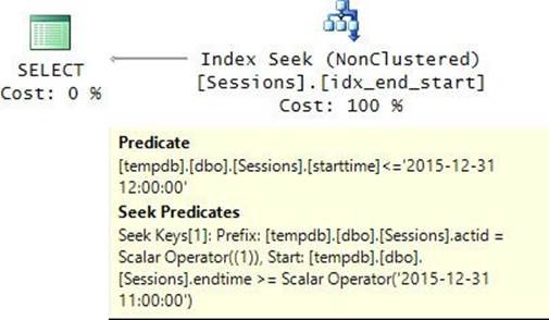
FIGURE 7-6 Interval intersection with index idx_end_start.
When I ran this query on my system, it performed only four logical reads!
When you’re done testing intersection queries, run the following code to drop the index idx_end_start (and keep the index idx_start_end for later examples):
DROP INDEX idx_end_start ON dbo.Sessions;
So, when you’re lucky enough to have most intersection queries applied to recent periods in your data, it’s easy to get good performance as long as you create the right index. However, if in your environment intersection queries can be applied to any period, you’re in trouble. Whether you create the index with starttime before endtime or the other way around, on average, every query will result in scanning half the rows for the account. The sample data I use has 200,000 rows per partition (account), so scanning half the rows is not necessarily a disaster, but what if you have millions per partition?
There’s a solution for intersection queries that works well in the more general cases. It is based on an ingenious model called the Relational Interval Tree (RI-tree) model. It was crafted by Hans-Peter Kriegel, Marco Pötke, and Thomas Seidl from the University of Munich, with further optimizations by Laurent Martin. The implementation of this model involves: (1) adding a column to the table representing what’s called the fork node in the model, (2) two B-tree-based indexes based on (forknode, starttime, key) and (forknode, endtime, key), and (3) new intersection queries that unify three disjoint sets of intersecting intervals, each using no more than one range predicate. This model and the improvements are downright beautiful and quite an impressive accomplishment. If you have the need to perform intersection queries in your application and you currently suffer from performance problems, it is certainly worthwhile getting familiar with it. You can find the details about the model, improvements, and implementation in SQL Server in the following resources:
![]() “Interval Queries in SQL Server” by Itzik Ben-Gan (http://sqlmag.com/t-sql/sql-server-interval-queries)
“Interval Queries in SQL Server” by Itzik Ben-Gan (http://sqlmag.com/t-sql/sql-server-interval-queries)
![]() “Managing Intervals Efficiently in Object-Relational Databases” by Hans-Peter Kriegel, Marco Pötke, and Thomas Seidl (http://www.dbs.ifi.lmu.de/Publikationen/Papers/VLDB2000.pdf)
“Managing Intervals Efficiently in Object-Relational Databases” by Hans-Peter Kriegel, Marco Pötke, and Thomas Seidl (http://www.dbs.ifi.lmu.de/Publikationen/Papers/VLDB2000.pdf)
![]() “A Static Relational Interval Tree” by Laurent Martin (http://www.solidq.com/static-relational-interval-tree/)
“A Static Relational Interval Tree” by Laurent Martin (http://www.solidq.com/static-relational-interval-tree/)
![]() “Advanced interval queries with the Static Relational Interval Tree” by Laurent Martin (http://www.solidq.com/advanced-interval-queries-static-relational-interval-tree/)
“Advanced interval queries with the Static Relational Interval Tree” by Laurent Martin (http://www.solidq.com/advanced-interval-queries-static-relational-interval-tree/)
![]() “Using the Static Relational Interval Tree with time intervals” by Laurent Martin (http://www.solidq.com/using-static-relational-interval-tree-time-intervals/)
“Using the Static Relational Interval Tree with time intervals” by Laurent Martin (http://www.solidq.com/using-static-relational-interval-tree-time-intervals/)
Max concurrent intervals
Finding the maximum number of concurrent intervals is a classic task. With our Sessions table, you need to compute for each account the maximum number of sessions that were active concurrently. Such calculations are usually done for reasons like figuring out peak use for capacity planning, billing purposes, and so on.
As usual, you need to know whether the interval delimiters are closed (exclusive) or open (inclusive). You need to know this to tell which intervals are considered active during any given point in time ts. For example, for a closed, closed interval [starttime, endtime] the interval is active during ts if ts >= starttime AND ts <= endtime. For a closed, open interval [starttime, endtime] the interval is active during ts if ts >= starttime AND ts < endtime. For the sake of this example, I’ll assume the latter (closed, open intervals).
For the small set of sample data, your solution should generate the following output:
actid mx
----------- -----------
1 2
2 3
3 2
I’ll start with a traditional yet inefficient set-based solution that is based on a subquery, and then I’ll continue with much more efficient solutions that are based on window functions.
The traditional subquery-based solution will benefit from the index idx_start_end you created earlier. If your Sessions table currently doesn’t have this index, create it by running the following code:
CREATE UNIQUE INDEX idx_start_end ON dbo.Sessions(actid, starttime, endtime, sessionid);
The solution starts by identifying the points in time when the maximum number of intervals potentially falls. If you follow the arrow of time, the count of active intervals changes only when an interval starts or ends. In between events, the count remains the same. Furthermore, every time an interval starts, the count increases; whereas every time an interval ends, the count decreases. Therefore, the maximum count has to fall on one of the start events. So the solution starts by defining a CTE called P that returns start-event time stamps (call the column ts) when the maximum count potentially falls:
WITH P AS -- time points
(
SELECT actid, starttime AS ts FROM dbo.Sessions
)
SELECT actid, ts FROM P;
The second step is to define a CTE called C with a query against P. The query uses a subquery to count the number of active intervals at ts for the same account based on the predicate I provided earlier. Here’s the code implementing this step:
WITH P AS -- time points
(
SELECT actid, starttime AS ts FROM dbo.Sessions
),
C AS -- counts
(
SELECT actid, ts,
(SELECT COUNT(*)
FROM dbo.Sessions AS S
WHERE P.actid = S.actid
AND P.ts >= S.starttime
AND P.ts < S.endtime) AS cnt
FROM P
)
SELECT actid, ts, cnt FROM C;
This code generates the following output using the small set of sample data:
actid ts cnt
------ -------------------- ----
1 2015-12-31 08:00:00 1
1 2015-12-31 08:30:00 1
1 2015-12-31 09:00:00 1
1 2015-12-31 10:00:00 1
1 2015-12-31 10:30:00 2
1 2015-12-31 11:30:00 2
2 2015-12-31 09:00:00 3
2 2015-12-31 08:30:00 2
2 2015-12-31 08:00:00 1
2 2015-12-31 11:00:00 1
2 2015-12-31 11:32:00 1
2 2015-12-31 12:04:00 1
3 2015-12-31 08:00:00 2
3 2015-12-31 08:00:00 2
3 2015-12-31 08:30:00 2
3 2015-12-31 09:30:00 0
![]() Note
Note
If you’re wondering how it can be that there are 0 active intervals at the last time stamp for account 3, that’s because the sample data has a degenerate interval with the same start time and end time. I wanted to include such an interval for examples involving closed, closed intervals like with the intersection test I discussed in the previous section. Currently, there’s a CHECK constraint that enforces the predicate endtime >= starttime to allow degenerate intervals. In practice, when your table will represent closed, open intervals and you won’t want to allow empty ones, your constraint will enforce this with the predicate endtime > starttime.
The third and final step is to group the rows from C by account and return the maximum count per account, like so:
WITH P AS -- time points
(
SELECT actid, starttime AS ts FROM dbo.Sessions
),
C AS -- counts
(
SELECT actid, ts,
(SELECT COUNT(*)
FROM dbo.Sessions AS S
WHERE P.actid = S.actid
AND P.ts >= S.starttime
AND P.ts < S.endtime) AS cnt
FROM P
)
SELECT actid, MAX(cnt) AS mx
FROM C
GROUP BY actid;
This solution is pretty simple and straightforward, so from a logical standpoint it’s alright. The problem is that it gets optimized very inefficiently even with the optimal index idx_start_end in place. The plan for this solution is shown in Figure 7-7.
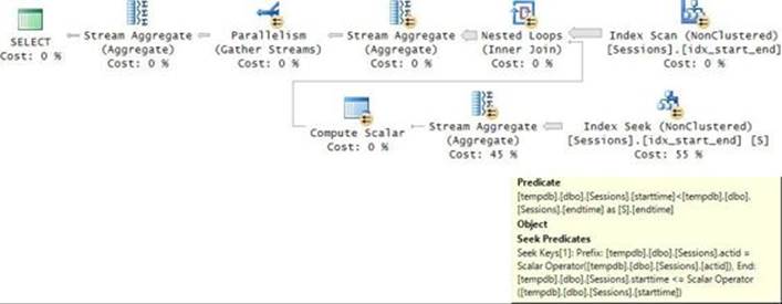
FIGURE 7-7 Plan for a traditional solution to the Max Concurrent Intervals task.
The outer branch of the Nested Loops join scans the index to get the time stamps against which you will compute the counts. You have as many time stamps as the number of intervals because those time stamps are the start points of all intervals. For each time stamp, the inner branch of the Nested Loops join performs a seek and a range scan in the index based on the predicate in the subquery: P.actid = S.actid AND P.ts >= S.starttime AND P.ts < S.endtime. Therein lies the problem. Thinking of the predicates from the perspective of the interval delimiters, you have two range predicates: S.starttime <= P.ts AND S.endtime > P.ts. On average, per time stamp, the Index Seek operator will scan about half the number of rows for the current account in the index leaf. With N rows per account, this means N2/2 rows are going to be scanned in total. Our table has 200,000 rows per account. This translates to 20,000,000,000 rows processed per account. On my system, it took about 11 minutes and 30 seconds to process one account. With 50 accounts, it takes the query about 10 hours to complete. What’s misleading in the plan that prevents you from seeing the excessive work is that the Index Seek operator doesn’t tell you how many rows it scanned; rather, it tells you how many rows it returned after applying all predicates.
When you’re done testing this solution, drop the index idx_start_end:
DROP INDEX idx_start_end ON dbo.Sessions;
There are much more efficient solutions to the Max Concurrent Intervals task, based on window functions. I’ll first provide a solution that is based on a window aggregate function with a frame, so it is supported only in SQL Server 2012 and later. I’ll then show a solution that is based on the ROW_NUMBER function, which is supported in earlier versions. Both solutions will benefit from the following indexes, which hold separate start and end events:
CREATE UNIQUE INDEX idx_start ON dbo.Sessions(actid, starttime, sessionid);
CREATE UNIQUE INDEX idx_end ON dbo.Sessions(actid, endtime, sessionid);
The first step in the solution is to generate the chronological sequence of events based on the order in which they happened. You mark start events with a +1 event type, meaning that the event increases the count of active intervals, and end events with a –1 because it decreases the count. Because the intervals in our example are open, closed ones, in cases where end and start events happen at the same time, you position end events before start events so that the count first drops before increasing. You achieve this by using type (ascending) as the tiebreaker after ts when you order the events. The following code implements the first step as a CTE called C1.
WITH C1 AS
(
SELECT actid, starttime AS ts, +1 AS type
FROM dbo.Sessions
UNION ALL
SELECT actid, endtime AS ts, -1 AS type
FROM dbo.Sessions
)
SELECT actid, ts, type
FROM C1
ORDER BY actid, ts, type;
This code generates the following output (only events for account 2 are shown):
actid ts type
----------- --------------------------- -----------
...
2 2015-12-31 08:00:00 1
2 2015-12-31 08:30:00 1
2 2015-12-31 09:00:00 1
2 2015-12-31 09:30:00 -1
2 2015-12-31 10:00:00 -1
2 2015-12-31 10:30:00 -1
2 2015-12-31 11:00:00 1
2 2015-12-31 11:30:00 -1
2 2015-12-31 11:32:00 1
2 2015-12-31 12:00:00 -1
2 2015-12-31 12:04:00 1
2 2015-12-31 12:30:00 -1
...
The second step computes the count of active intervals after each event simply as the running total type over time. Here’s the code implementing the second step as a CTE called C2:
WITH C1 AS
(
SELECT actid, starttime AS ts, +1 AS type
FROM dbo.Sessions
UNION ALL
SELECT actid, endtime AS ts, -1 AS type
FROM dbo.Sessions
),
C2 AS
(
SELECT *,
SUM(type) OVER(PARTITION BY actid
ORDER BY ts, type
ROWS UNBOUNDED PRECEDING) AS cnt
FROM C1
)
SELECT actid, ts, type, cnt FROM C2;
This step generates the following output (for account 2):
actid ts type cnt
------ -------------------- ----- ----
...
2 2015-12-31 08:00:00 1 1
2 2015-12-31 08:30:00 1 2
2 2015-12-31 09:00:00 1 3
2 2015-12-31 09:30:00 -1 2
2 2015-12-31 10:00:00 -1 1
2 2015-12-31 10:30:00 -1 0
2 2015-12-31 11:00:00 1 1
2 2015-12-31 11:30:00 -1 0
2 2015-12-31 11:32:00 1 1
2 2015-12-31 12:00:00 -1 0
2 2015-12-31 12:04:00 1 1
2 2015-12-31 12:30:00 -1 0
...
Then the final step is just to group the rows from C2 by account and return the maximum count for each group, like so:
WITH C1 AS
(
SELECT actid, starttime AS ts, +1 AS type
FROM dbo.Sessions
UNION ALL
SELECT actid, endtime AS ts, -1 AS type
FROM dbo.Sessions
),
C2 AS
(
SELECT *,
SUM(type) OVER(PARTITION BY actid
ORDER BY ts, type
ROWS UNBOUNDED PRECEDING) AS cnt
FROM C1
)
SELECT actid, MAX(cnt) AS mx
FROM C2
GROUP BY actid;
The execution plan for this query is shown in Figure 7-8.
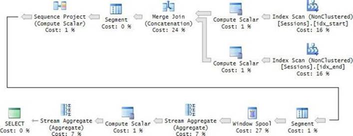
FIGURE 7-8 Plan for a solution with a window aggregate function to the Max Concurrent Intervals task.
The plan is quite efficient. The indexes idx_start and idx_end are both scanned in order; the rows are merged, preserving the order. Then both the window aggregate and the group aggregate are computed based on that order. No sort operations are applied in the plan. The query took 44 seconds to complete on my system and has linear scaling. That’s not too bad considering that the traditional solution with the subquery took 10 hours to complete.
Another solution to the task is based on the ROW_NUMBER function. It has two advantages over the solution with the window aggregate. Remember that window aggregates with a frame option are available only in SQL Server 2012 and later, whereas window ranking functions were available earlier. Also, window aggregate functions use the Window Spool operator to spool the frame of rows, which is extra work. The ROW_NUMBER function uses streaming operators to handle the computation with no spooling. So handling the task with the ROW_NUMBER function results in better performance.
The solution based on the ROW_NUMBER function starts similarly to the solution based on the window aggregate. It generates the chronological sequence of events by unifying start and end events. In addition, it computes two row numbers: one that counts how many start events happened until the current start event (call it s), and another computing how many start and end events happened until the current start or end event (call it se). You compute the ordinal s in the query that returns start events, and you return a NULL as a placeholder in the parallel column in the query that returns end events. You define a CTE called C1 representing the unified chronological sequence of events including the ordinal s. Then you query C1 and compute the ordinal se against the unified events. You define a CTE called C2 based on this query, giving you the unified chronological sequence of events, including both ordinals s and se. Here’s the code implementing the first step:
WITH C1 AS
(
SELECT actid, starttime AS ts, +1 AS type, sessionid,
ROW_NUMBER() OVER(PARTITION BY actid ORDER BY starttime, sessionid) AS s
FROM dbo.Sessions
UNION ALL
SELECT actid, endtime AS ts, -1 AS type, sessionid, NULL AS s
FROM dbo.Sessions
),
C2 AS
(
SELECT *,
ROW_NUMBER() OVER(PARTITION BY actid ORDER BY ts, type, sessionid) AS se
FROM C1
)
SELECT sessionid, actid, ts, type, s, se FROM C2;
This code generates the following output (only events for account 2 are shown here):
sessionid actid ts type s se
---------- ------ --------------------- ----- ----- ---
...
7 2 2015-12-31 08:00:00 1 1 1
8 2 2015-12-31 08:30:00 1 2 2
9 2 2015-12-31 09:00:00 1 3 3
9 2 2015-12-31 09:30:00 -1 NULL 4
8 2 2015-12-31 10:00:00 -1 NULL 5
7 2 2015-12-31 10:30:00 -1 NULL 6
10 2 2015-12-31 11:00:00 1 4 7
10 2 2015-12-31 11:30:00 -1 NULL 8
11 2 2015-12-31 11:32:00 1 5 9
11 2 2015-12-31 12:00:00 -1 NULL 10
12 2 2015-12-31 12:04:00 1 6 11
12 2 2015-12-31 12:30:00 -1 NULL 12
...
Recall that the maximum count necessarily falls on one of the start events; that’s why it’s not interesting to compute counts near end events. You now know for each start event how many start events happened so far (s) and how many start and end events happened so far (se). Based on these two, you compute how many end events happened so far simply as se – s. Then the count of active intervals is the count of start events so far (s) minus the count of end events so far (se – s), namely s – (se – s). You compute this count (call it cnt) in a query against the CTE C2. Then the final step is to group the rows by account and compute the maximum count per group, like so:
WITH C1 AS
(
SELECT actid, starttime AS ts, +1 AS type, sessionid,
ROW_NUMBER() OVER(PARTITION BY actid ORDER BY starttime, sessionid) AS s
FROM dbo.Sessions
UNION ALL
SELECT actid, endtime AS ts, -1 AS type, sessionid, NULL AS s
FROM dbo.Sessions
),
C2 AS
(
SELECT *,
ROW_NUMBER() OVER(PARTITION BY actid ORDER BY ts, type, sessionid) AS se
FROM C1
)
SELECT actid, MAX(cnt) AS mx
FROM C2
CROSS APPLY ( VALUES( s - (se - s) ) ) AS A(cnt)
GROUP BY actid;
The plan for this query is shown in Figure 7-9.
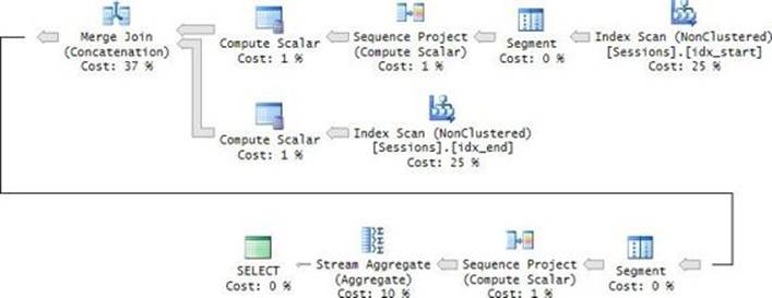
FIGURE 7-9 Plan for a solution with a ROW_NUMBER function to the Max Concurrent Intervals task.
The two indexes idx_start and idx_end are scanned in order. The ordinal s is computed by the Segment and Sequence Project operators based on the order of the start events. The start and end events are merged, preserving the order. Another pair of Segment and Sequence Project operators compute the ordinal se based on that order. Finally, a Stream Aggregate operator handles the group count, still relying on that order. No explicit sort operations are required. The advantage of this plan is that there’s no spooling, unlike in the plan for the previous solution. The Sequence Project operator, which computes the row numbers, is a streaming operator. It would certainly be nice to see future improvements in SQL Server’s optimization of aggregate window functions handling common calculations like running totals with streaming operators instead of spooling ones. This plan completed in 17 seconds on my system.
You can further improve the performance of the solution by enabling parallel treatment for different accounts. Encapsulate the logic for a single account in an inline TVF, like so:
IF OBJECT_ID(N'dbo.MaxConcurrent', N'IF') IS NOT NULL
DROP FUNCTION dbo.MaxConcurrent;
GO
CREATE FUNCTION dbo.MaxConcurrent( @actid AS INT ) RETURNS TABLE
AS
RETURN
WITH C1 AS
(
SELECT starttime AS ts, +1 AS type, sessionid,
ROW_NUMBER() OVER(ORDER BY starttime, sessionid) AS s
FROM dbo.Sessions
WHERE actid = @actid
UNION ALL
SELECT endtime AS ts, -1 AS type, sessionid, NULL AS s
FROM dbo.Sessions
WHERE actid = @actid
),
C2 AS
(
SELECT *,
ROW_NUMBER() OVER(ORDER BY ts, type, sessionid) AS se
FROM C1
)
SELECT MAX(cnt) AS mx
FROM C2
CROSS APPLY ( VALUES( s - (se - s) ) ) AS A(cnt);
GO
Query the Accounts table, and using the CROSS APPLY operator apply the inline TVF to each account, like so (trace flag 8649 is used to get a parallel plan for demonstration purposes):
SELECT A.actid, C.mx
FROM dbo.Accounts AS A
CROSS APPLY dbo.MaxConcurrent(A.actid) AS C
OPTION(QUERYTRACEON 8649);
I got the plan shown in Figure 7-10 for this query.
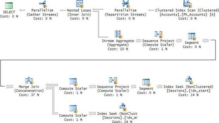
FIGURE 7-10 Solution to the Max Concurrent Intervals task with improved parallelism.
The outer branch of the Nested Loops join scans the Accounts table with a parallel scan, and then it uses the Repartition Streams operator to distribute the work to the different threads using a round-robin algorithm. This results in the inner branch of the Nested Loops join doing work for one account per thread from the outer branch. So even though each account is handled by one thread, multiple accounts are handled in parallel. This plan took eight seconds to complete on my system. That’s quite amazing compared to the 10-hour run time of the first solution.
Packing intervals
Packing is another classic task involving intervals. The idea is to merge all intervals that intersect into one packed interval. With our sample data, you’re supposed to pack the intervals in the Sessions table per account so that you get the contiguous intervals in which each account had active sessions, never mind how many.
For example, suppose a certain account has the following intervals: [p1, p4), [p2, p3), [p4, p7), [p9, p12), and [p12, p14). The packed intervals are [p1, p7) and [p9, p14). Observe that if one interval starts when another ends, the two are packed together. Following is the desired result for packing the intervals represented by the small set of sample data in the Sessions table:
actid starttime endtime
----------- --------------------------- ---------------------------
1 2015-12-31 08:00:00 2015-12-31 09:30:00
1 2015-12-31 10:00:00 2015-12-31 12:30:00
2 2015-12-31 08:00:00 2015-12-31 10:30:00
2 2015-12-31 11:00:00 2015-12-31 11:30:00
2 2015-12-31 11:32:00 2015-12-31 12:00:00
2 2015-12-31 12:04:00 2015-12-31 12:30:00
3 2015-12-31 08:00:00 2015-12-31 09:00:00
3 2015-12-31 09:30:00 2015-12-31 09:30:00
Like with the Max Concurrent Intervals task, the Packing task also has older, traditional solutions that perform very badly and much faster, newer solutions based on window functions. I’ll spare you from going over the traditional solutions and jump straight to the efficient ones. Indexing guidelines are the same as before—namely, create separate indexes for start and end events. If you currently don’t have the indexes idx_start and idx_end defined on the Sessions table, run the following code to create those:
CREATE UNIQUE INDEX idx_start ON dbo.Sessions(actid, starttime, sessionid);
CREATE UNIQUE INDEX idx_end ON dbo.Sessions(actid, endtime, sessionid);
You handle the Packing task based on concepts similar to the ones used in the solutions for the Max Concurrent Intervals task, but with a few extra complexities on top. Also, with packing you rely on computing counts of active intervals, and you can compute those counts either using a window aggregate function or using the ROW_NUMBER function. I’ll first describe the solution using a window aggregate.
The first step is to generate a unified chronological sequence of events with a +1 type marking start events and a –1 type marking end events. You define a CTE called C1 based on the query that implements this step.
The second step is to compute the count of active intervals by applying a running sum of the type column. However, there are two things that are different about the running sum calculation in the Packing task compared to the Max Concurrent Intervals task. One is that in the window order clause you use type DESC as the tiebreaker after ts for start and end events that happen at the same time. That’s because when packing intervals, you want such events to be part of the same packed interval, and by placing start events before end events, you ensure that the count doesn’t drop to zero during a packed interval. The second thing that is different is that when the event is a start event, you need to subtract 1 from the count because for packing purposes, it needs to reflect how many intervals were active before the event was applied. With end events, you actually do need the count to reflect the state after the event was applied, so there’s no need to subtract anything in such a case. The subtraction logic can be handled with a CASE expression. You define a CTE called C2 based on the query that implements the second step. Here’s the code handling the first two steps:
WITH C1 AS
(
SELECT sessionid, actid, starttime AS ts, +1 AS type
FROM dbo.Sessions
UNION ALL
SELECT sessionid, actid, endtime AS ts, -1 AS type
FROM dbo.Sessions
),
C2 AS
(
SELECT *,
SUM(type) OVER(PARTITION BY actid
ORDER BY ts, type DESC
ROWS UNBOUNDED PRECEDING)
- CASE WHEN type = 1 THEN 1 ELSE 0 END AS cnt
FROM C1
)
SELECT sessionid, actid, ts, type, cnt FROM C2;
This code generates the following output for account 2:
sessionid actid ts type cnt
---------- ------ -------------------- ----------- -----------
...
7 2 2015-12-31 08:00:00 1 0
8 2 2015-12-31 08:30:00 1 1
9 2 2015-12-31 09:00:00 1 2
9 2 2015-12-31 09:30:00 -1 2
8 2 2015-12-31 10:00:00 -1 1
7 2 2015-12-31 10:30:00 -1 0
10 2 2015-12-31 11:00:00 1 0
10 2 2015-12-31 11:30:00 -1 0
11 2 2015-12-31 11:32:00 1 0
11 2 2015-12-31 12:00:00 -1 0
12 2 2015-12-31 12:04:00 1 0
12 2 2015-12-31 12:30:00 -1 0
...
The third step is to filter only events that represent start and end points of a packed interval. Those are the events where cnt is zero. Once filtered, each consecutive pair of events represents a packed interval. You need to compute a pair identifier (call it p) so that you can handle each pair as a group. For this purpose, you compute a row number (call it rn), and then p is computed as FLOOR( (rn + 1) / 2 ).
![]() Note
Note
In T-SQL, you don’t need to explicitly floor the result of the calculation because with integer inputs, you will get integer division. But in other platforms, like Oracle, you get numeric division by default, and the FLOOR function is required for the calculation to be correct. Because I wanted the solution to be more portable, I used this form even though in SQL Server the FLOOR function is unnecessary.
You define a CTE called C3 based on the query that implements this step.
Finally, you query C3, group the rows by the account and pair identifier, and then return the minimum time stamp as the start of the packed interval and the maximum time stamp as the end. Here’s the complete solution code:
WITH C1 AS
(
SELECT sessionid, actid, starttime AS ts, +1 AS type
FROM dbo.Sessions
UNION ALL
SELECT sessionid, actid, endtime AS ts, -1 AS type
FROM dbo.Sessions
),
C2 AS
(
SELECT *,
SUM(type) OVER(PARTITION BY actid
ORDER BY ts, type DESC
ROWS UNBOUNDED PRECEDING)
- CASE WHEN type = 1 THEN 1 ELSE 0 END AS cnt
FROM C1
),
C3 AS
(
SELECT *,
FLOOR((ROW_NUMBER() OVER(PARTITION BY actid ORDER BY ts) + 1) / 2) AS p
FROM C2
WHERE cnt = 0
)
SELECT actid, MIN(ts) AS starttime, max(ts) AS endtime
FROM C3
GROUP BY actid, p;
This query took 54 seconds to complete on my system.
Just like with the Max Concurrent Intervals task, with the Packing task you can compute the count of concurrent intervals using the ROW_NUMBER function more efficiently than using a window aggregate function. For packing purposes, you will need to apply a few adjustments to the previous calculations, but the general idea is pretty similar.
One adjustment is to the calculation of the ordinal se, which counts start and end events. Remember that for packing purposes, in case start and end events happen at the same time, they are considered part of the same packed interval. For this reason, in the window order clause of the ROW_NUMBER function computing se, you specify type DESC (as opposed to the ascending direction used before) as the tiebreaker after ts, not allowing the count to drop to zero during a packed interval.
Another adjustment is to the calculation of the counts near start events (what was called cnt before and will now be referred to as cs). For packing purposes, you need the count to reflect the state before the start event was applied. So you need to subtract 1 from the previous calculation, giving you s – (se – s) – 1.
Another adjustment is that, unlike in the previous task where you needed counts only near start events, with packing you also need the counts near end events (call the column ce). For this purpose, you will apply a symmetric calculation to cs. This means you will compute a row number counting end events (call it e) in the query retrieving end events, and you will use a NULL as a placeholder in the query retrieving start events. Then you will compute ce based on e and se as (se – e) – e.
Once you have cs and ce computed, you handle the filtering of only events representing start and end points of packed intervals by using the predicate cs = 0 OR ce = 0. The rest of the solution is the same as in the solution based on the window aggregate function; namely, you compute the pair identifier (p), group the rows by account and pair identifier, and return the minimum and maximum time stamps as the start and end of the packed interval.
Here’s the complete solution code:
WITH C1 AS
(
SELECT sessionid, actid, starttime AS ts, +1 AS type,
ROW_NUMBER() OVER(PARTITION BY actid ORDER BY starttime, sessionid) AS s,
NULL AS e
FROM dbo.Sessions
UNION ALL
SELECT sessionid, actid, endtime AS ts, -1 AS type,
NULL AS s,
ROW_NUMBER() OVER(PARTITION BY actid ORDER BY endtime, sessionid) AS e
FROM dbo.Sessions
),
C2 AS
(
SELECT *,
ROW_NUMBER() OVER(PARTITION BY actid ORDER BY ts, type DESC, sessionid) AS se
FROM C1
),
C3 AS
(
SELECT *,
FLOOR((ROW_NUMBER() OVER(PARTITION BY actid ORDER BY ts) + 1) / 2) AS p
FROM C2
CROSS APPLY ( VALUES(s - (se - s) - 1, (se - e) - e) ) AS A(cs, ce)
WHERE cs = 0 OR ce = 0
)
SELECT actid, MIN(ts) AS starttime, MAX(ts) AS endtime
FROM C3
GROUP BY actid, p;
The plan for this solution is shown in Figure 7-11.
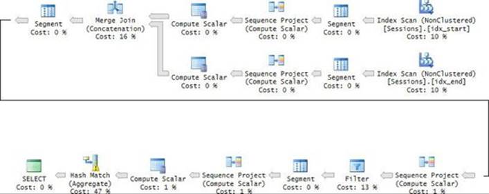
FIGURE 7-11 Plan for a solution based on ROW_NUMBER to the Packing task.
This solution completed in 26 seconds on my system.
Just like with the previous task, with the Packing task you can further improve parallelism handling by encapsulating the work for a single account in an inline TVF and then applying the TVF to the Accounts table using the APPLY operator. Run the following code to define the inline TVF:
IF OBJECT_ID(N'dbo.PackedIntervals', N'IF') IS NOT NULL DROP FUNCTION dbo.PackedIntervals;
GO
CREATE FUNCTION dbo.PackedIntervals( @actid AS INT ) RETURNS TABLE
AS
RETURN
WITH C1 AS
(
SELECT sessionid, starttime AS ts, +1 AS type,
ROW_NUMBER() OVER(ORDER BY starttime, sessionid) AS s,
NULL AS e
FROM dbo.Sessions
WHERE actid = @actid
UNION ALL
SELECT sessionid, endtime AS ts, -1 AS type,
NULL AS s,
ROW_NUMBER() OVER(ORDER BY endtime, sessionid) AS e
FROM dbo.Sessions
WHERE actid = @actid
),
C2 AS
(
SELECT *,
ROW_NUMBER() OVER(ORDER BY ts, type DESC, sessionid) AS se
FROM C1
),
C3 AS
(
SELECT *,
FLOOR((ROW_NUMBER() OVER(ORDER BY ts) + 1) / 2) AS p
FROM C2
CROSS APPLY ( VALUES(s - (se - s) - 1, (se - e) - e) ) AS A(cs, ce)
WHERE cs = 0 OR ce = 0
)
SELECT MIN(ts) AS starttime, MAX(ts) AS endtime
FROM C3
GROUP BY p;
GO
Then use the following query to apply the TVF to the Accounts table (again, TF 8649 is used to force parallelism for demonstration purposes):
SELECT A.actid, P.starttime, P.endtime
FROM dbo.Accounts AS A
CROSS APPLY dbo.PackedIntervals(A.actid) AS P
OPTION(QUERYTRACEON 8649);
Figure 7-12 has the plan that I got for this query on my system.
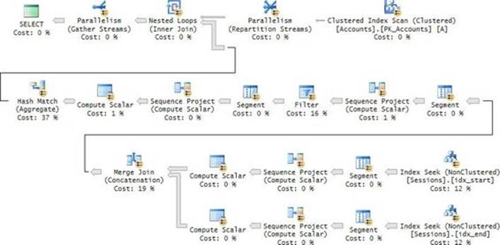
FIGURE 7-12 Plan for a solution to the Packing task with improved parallelism.
This query took only 10 seconds to complete on my system.
Conclusion
As you can see, there’s a lot of trickiness in dealing with date and time data. There are pitfalls related to different language conventions, rounding problems, nonSARGable filters, and limitations of the implementation. Fortunately, there are solutions you can use to handle date and time related tasks correctly and efficiently, even though some of those solutions are more complex and require some creativity. This chapter gave you an appreciation of the importance of following best practices and the tools to do your job well as far as handling of date and time data is concerned.