CCNP Routing and Switching ROUTE 300-101 Official Cert Guide (2015)
Part I. Fundamental Routing Concepts
Chapter 1. Characteristics of Routing Protocols
This chapter covers the following subjects:
![]() Routing Protocol Fundamentals: This section offers an overview of the role that routing plays in an enterprise network and contrasts various types of routing protocols.
Routing Protocol Fundamentals: This section offers an overview of the role that routing plays in an enterprise network and contrasts various types of routing protocols.
![]() Network Technology Fundamentals: This section distinguishes between different types of network traffic flows and network architectures.
Network Technology Fundamentals: This section distinguishes between different types of network traffic flows and network architectures.
![]() TCP/IP Fundamentals: This section reviews the fundamental characteristics of IP, ICMP, TCP, and UDP.
TCP/IP Fundamentals: This section reviews the fundamental characteristics of IP, ICMP, TCP, and UDP.
![]() Network Migration Strategies: This section offers a collection of design considerations for making changes to a network.
Network Migration Strategies: This section offers a collection of design considerations for making changes to a network.
One of the most fundamental technologies in network is routing. Routing, at its essence, is concerned with forwarding packets from their source on one subnet to their destination on another subnet. Of course, a multitude of options and protocols are available for making this happen. In fact, routing is the theme of this entire book, the focus of Cisco’s ROUTE course, and the accompanying ROUTE exam (300-101).
This chapter launches the discussion of routing by providing a conceptual introduction. Specifically, this chapter begins with a discussion of routing protocol fundamentals, followed by the basics of network technology and the TCP/IP suite of protocols.
The chapter then concludes with a design discussion revolving around how to accommodate the inevitable changes your network will undergo. For example, you will be given a collection of strategies for changing routing protocols in your network or migrating from IPv4 to IPv6.
“Do I Know This Already?” Quiz
The “Do I Know This Already?” quiz allows you to assess whether you should read the entire chapter. If you miss no more than one of these eight self-assessment questions, you might want to move ahead to the “Exam Preparation Tasks” section. Table 1-1 lists the major headings in this chapter and the “Do I Know This Already?” quiz questions covering the material in those headings so that you can assess your knowledge of these specific areas. The answers to the “Do I Know This Already?” quiz appear in Appendix A.
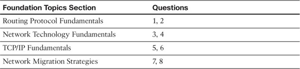
Table 1-1 “Do I Know This Already?” Foundation Topics Section-to-Question Mapping
1. Which of the following features prevents a route learned on one interface from being advertised back out of that interface?
a. Poison Reverse
b. Summarization
c. Split Horizon
d. Convergence
2. Identify the distance-vector routing protocols from the following. (Choose the two best answers.)
a. IS-IS
b. EIGRP
c. RIP
d. OSPF
e. BGP
3. Select the type of network communication flow that is best described as “one-to-nearest.”
a. Unicast
b. Multicast
c. Broadcast
d. Anycast
4. An NBMA network has which of the following design issues? (Choose the two best answers.)
a. Split Horizon issues
b. Bandwidth issues
c. Quality of service issues
d. Designated router issues
5. Which of the following best defines TCP MSS?
a. The total data in a TCP segment, including only the TCP header
b. The total data in a TCP segment, not including any headers
c. The total data in a TCP segment, including only the IP and TCP headers
d. The total data in a TCP segment, including the Layer 2, IP, and TCP headers
6. A network segment has a bandwidth of 10 Mbps, and packets experience an end-to-end latency of 100 ms. What is the bandwidth-delay product of the network segment?
a. 100,000,000 bits
b. 10,000,000 bits
c. 1,000,000 bits
d. 100,000 bits
7. When migrating from a PVST+ to Rapid-PVST+, which PVST+ features can be disabled, because similar features are built into Rapid-PVST+? (Choose the two best answers.)
a. UplinkFast
b. Loop Guard
c. BackboneFast
d. PortFast
8. Cisco EVN uses what type of trunk to carry traffic for all virtual networks between two physical routers?
a. VNET
b. ISL
c. dot1Q
d. 802.10
Foundation Topics
Routing Protocol Fundamentals
Routing occurs when a router or some other Layer 3 device (for example, a multilayer switch) makes a forwarding decision based on network address information (that is, Layer 3 information). A fundamental question, however, addressed throughout this book, is from where does the routing information originate?
A router could know how to reach a network by simply having one of its interfaces directly connect that network. Perhaps you statically configured a route, telling a router exactly how to reach a certain destination network. However, for large enterprises, the use of static routes does not scale well. Therefore, dynamic routing protocols are typically seen in larger networks (and many small networks, too). A dynamic routing protocol allows routers configured for that protocol to exchange route information and update that information based on changing network conditions.
The first topic in this section explores the role of routing in an enterprise network. Then some of the characteristics of routing protocols are presented, to help you decide which routing protocol to use in a specific environment and to help you better understand the nature of routing protocols you find already deployed in a network.
The Role of Routing in an Enterprise Network
An enterprise network typically interconnects multiple buildings, has connectivity to one or more remote offices, and has one or more connections to the Internet. Figure 1-1 identifies some of the architectural layers often found in an enterprise network design:
![]() Building Access: This layer is part of the Campus network and is used to provide user access to the network. Security (especially authentication) is important at this layer, to verify that a user should have access to the network. Layer 2 switching is typically used at this layer, in conjunction with VLANs.
Building Access: This layer is part of the Campus network and is used to provide user access to the network. Security (especially authentication) is important at this layer, to verify that a user should have access to the network. Layer 2 switching is typically used at this layer, in conjunction with VLANs.
![]() Building Distribution: This layer is part of the Campus network that aggregates building access switches. Multilayer switches are often used here.
Building Distribution: This layer is part of the Campus network that aggregates building access switches. Multilayer switches are often used here.
![]() Campus Backbone: This layer is part of the Campus network and is concerned with the high-speed transfer of data through the network. High-end multilayer switches are often used here.
Campus Backbone: This layer is part of the Campus network and is concerned with the high-speed transfer of data through the network. High-end multilayer switches are often used here.
![]() Edge Distribution: This layer is part of the Campus network and serves as the ingress and egress point for all traffic into and out of the Campus network. Routers or multilayer switches are appropriate devices for this layer.
Edge Distribution: This layer is part of the Campus network and serves as the ingress and egress point for all traffic into and out of the Campus network. Routers or multilayer switches are appropriate devices for this layer.
![]() Internet Gateways: This layer contains routers that connect the Campus network out to the Internet. Some enterprise networks have a single connection out to the Internet, while others have multiple connections out to one or more Internet Service Providers (ISP).
Internet Gateways: This layer contains routers that connect the Campus network out to the Internet. Some enterprise networks have a single connection out to the Internet, while others have multiple connections out to one or more Internet Service Providers (ISP).
![]() WAN Aggregation: This layer contains routers that connect the Campus network out to remote offices. Enterprises use a variety of WAN technologies to connect to remote offices (for example, Multiprotocol Label Switching [MPLS]).
WAN Aggregation: This layer contains routers that connect the Campus network out to remote offices. Enterprises use a variety of WAN technologies to connect to remote offices (for example, Multiprotocol Label Switching [MPLS]).
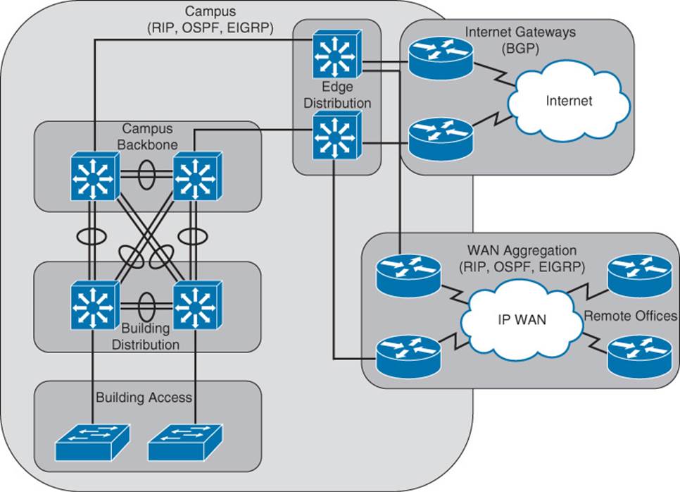
Figure 1-1 Typical Components of an Enterprise Network
Routing protocols used within the Campus network and within the WAN aggregation layer are often versions of Routing Information Protocol (RIP), Open Shortest Path First (OSPF), or Enhanced Interior Gateway Routing Protocol (EIGRP). However, when connecting out to the Internet, Border Gateway Protocol (BGP) is usually the protocol of choice for enterprises having more than one Internet connection.
An emerging industry trend is to connect a campus to a remote office over the Internet, as opposed to using a traditional WAN technology. Of course, the Internet is considered an untrusted network, and traffic might need to traverse multiple routers on its way from the campus to a remote office. However, a technology called Virtual Private Networks (VPN) allows a logical connection to be securely set up across an Internet connection. Chapter 2, “Remote Site Connectivity,” examines VPNs in more detail.
Routing Protocol Selection
As you read through this book, you will learn about the RIPv2, RIPng, OSPFv2, OSPFv3, EIGRP, BGP, and MP-BGP routing protocols. With all of these choices (and even more) available, a fundamental network design consideration becomes which routing protocol to use in your network. As you learn more about these routing protocols, keeping the following characteristics in mind can help you do a side-by-side comparison of protocols:
![]() Scalability
Scalability
![]() Vendor interoperability
Vendor interoperability
![]() IT staff’s familiarity with protocol
IT staff’s familiarity with protocol
![]() Speed of convergence
Speed of convergence
![]() Capability to perform summarization
Capability to perform summarization
![]() Interior or exterior routing
Interior or exterior routing
![]() Type of routing protocol
Type of routing protocol
This section of the chapter concludes by taking a closer look at each of these characteristics.
Scalability
How large is your network now, and how large is it likely to become? The answers to those questions can help determine which routing protocols not to use in your network. For example, while you could use statically configured routes in a network with just a couple of routers, such a routing solution does not scale well to dozens of routers.
While all the previously mentioned dynamic routing protocols are capable of supporting most medium-sized enterprise networks, you should be aware of any limitations. For example, all versions of RIP have a maximum hop count (that is, the maximum number of routers across which routing information can be exchanged) of 15 routers. BGP, on the other hand, is massively scalable. In fact, BGP is the primary routing protocol used on the Internet.
Vendor Interoperability
Will you be using all Cisco routers in your network, or will your Cisco routers need to interoperate with non-Cisco routers? A few years ago, the answer to this question could be a deal-breaker for using EIGRP, because EIGRP was a Cisco-proprietary routing protocol.
However, in early 2013, Cisco announced that it was releasing EIGRP to the Internet Engineering Task Force (IETF) standards body as an Informational RFC. As a result, any networking hardware vendor can use EIGRP on its hardware. If you are working in an environment with routers from multiple vendors, you should ensure that your Cisco router has an appropriate Cisco IOS feature set to support your desired routing protocol and that the third-party router(s) also support that routing protocol.
IT Staff’s Familiarity with Protocol
You and the IT staff at your company (or your customer’s company) might be much more familiar with one routing protocol than another. Choosing the routing protocol with which the IT staff is more familiar could reduce downtime (because of faster resolutions to troubleshooting issues). Also, if the IT staff is more familiar with the inner workings of one routing protocol, they would be more likely to take advantage of the protocol’s nontrivial features and tune the protocol’s parameters for better performance.
Speed of Convergence
A benefit of dynamic routing protocols over statically configured routes is the ability of a dynamic routing protocol to reroute around a network failure. For example, consider Figure 1-2. Router R1’s routing protocol might have selected the path through Router R3 as the best route to reach the 192.168.1.0 /24 network connected to Router R4. However, imagine that a link failure occurred on the Fast Ethernet link between Routers R3 and R4. Router R1’s routing protocol should be able to reroute around the link failure by sending packets destined for the 192.168.1.0 /24 network through Router R2.
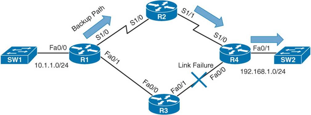
Figure 1-2 Routing Protocol Convergence
After this failover occurs, and the network reaches a steady-state condition (that is, the routing protocol is aware of current network conditions and forwards traffic based on those conditions), the network is said to be a converged network. The amount of time for the failover to occur is called the convergence time.
Some routing protocols have faster convergence times than others. RIP and BGP, for example, might take a few minutes to converge, depending on the network topology. By contrast, OSPF and EIGRP can converge in just a few seconds.
Capability to Perform Summarization
Large enterprise networks can have routing tables with many route entries. The more entries a router maintains in its routing table, the more router CPU resources are required to calculate the best path to a destination network. Fortunately, many routing protocols support the ability to do network summarization, although the summarization options and how summarization is performed do differ.
Network summarization allows multiple routes to be summarized in a single route advertisement. Not only does summarization reduce the number of entries in a router’s routing table, but it also reduces the number of network advertisements that need to be sent.
Figure 1-3 shows an example of route summarization. Specifically, Router R1 is summarizing the 10.0.0.0 /24, 10.0.1.0 /24, 10.0.2.0 /24, and 10.0.3.0 /24 networks into a single network advertisement of 10.0.0.0 /22. Notice that the first two octets (and therefore the first 16 bits) of all the networks are the same. Also, as shown in the figure, the first 6 bits in the third octet are the same for all the networks. Therefore, all the networks have the first 22 bits (that is, 16 bits in the first two octets plus 6 bits in the third octet) in common. By using those 22 bits and setting the remaining bits to 0s, you find the network address, 10.0.0.0 /22.

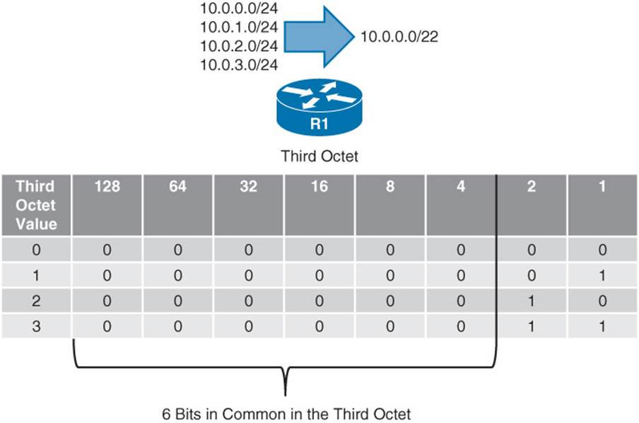
Figure 1-3 Network Summarization
Interior or Exterior Routing
An autonomous system (AS) is a network under a single administrative control. Your company’s network, as an example, might be in a single AS. When your company connects out to two different ISPs, they are each in their own AS. Figure 1-4 shows such a topology.
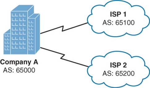
Figure 1-4 Interconnection of Autonomous Systems
In Figure 1-4, Company A is represented with an AS number of 65000. ISP 1 is using an AS number of 65100, and ISP 2 has an AS number of 65200.
When selecting a routing protocol, you need to determine where the protocol will run. Will it run within an autonomous system or between autonomous systems? The answer to that question determines whether you need an interior gateway protocol (IGP) or an exterior gateway protocol (EGP):
![]() IGP: An IGP exchanges routes between routers in a single AS. Common IGPs include OSPF and EIGRP. Although less popular, RIP and IS-IS are also considered IGPs. Also, be aware that BGP is used as an EGP; however, you can use interior BGP (iBGP) within an AS.
IGP: An IGP exchanges routes between routers in a single AS. Common IGPs include OSPF and EIGRP. Although less popular, RIP and IS-IS are also considered IGPs. Also, be aware that BGP is used as an EGP; however, you can use interior BGP (iBGP) within an AS.
![]() EGP: Today, the only EGP in use is BGP. However, from a historical perspective, be aware that there was once another EGP, which was actually named Exterior Gateway Protocol (EGP).
EGP: Today, the only EGP in use is BGP. However, from a historical perspective, be aware that there was once another EGP, which was actually named Exterior Gateway Protocol (EGP).
Routing Protocol Categories
Another way to categorize a routing protocol is based on how it receives, advertises, and stores routing information. The three fundamental approaches are distance-vector, link-state, and path-vector.
Distance-Vector
A distance-vector routing protocol sends a full copy of its routing table to its directly attached neighbors. This is a periodic advertisement, meaning that even if there have been no topological changes, a distance-vector routing protocol will, at regular intervals, re-advertise its full routing table to its neighbors.
Obviously, this periodic advertisement of redundant information is inefficient. Ideally, you want a full exchange of route information to occur only once and subsequent updates to be triggered by topological changes.
Another drawback to distance-vector routing protocols is the time they take to converge, which is the time required for all routers to update their routing table in response to a topological change in a network. Hold-down timers can speed the convergence process. After a router makes a change to a route entry, a hold-down timer prevents any subsequent updates for a specified period of time. This approach helps stop flapping routes (which are routes that oscillate between being available and unavailable) from preventing convergence.
Yet another issue with distance-vector routing protocols is the potential of a routing loop. To illustrate, consider Figure 1-5. In this topology, the metric being used is hop count, which is the number of routers that must be crossed to reach a network. As one example, Router R3’s routing table has a route entry for network 10.1.1.0 /24 available off of Router R1. For Router R3 to reach that network, two routers must be transited (Routers R2 and R1). As a result, network 10.1.1.0 /24 appears in Router R3’s routing table with a metric (hop count) of 2.
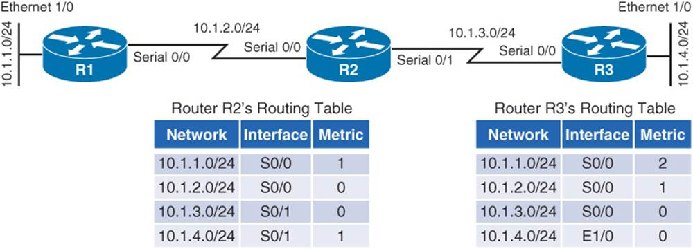
Figure 1-5 Routing Loop: Before Link Failure
Continuing with the example, imagine that interface Ethernet 1/0 on Router R3 goes down. As shown in Figure 1-6, Router R3 loses its directly connected route (with a metric of 0) to network 10.1.4.0 /24; however, Router R2 had a route to 10.1.4.0 /24 in its routing table (with a metric of 1), and this route was advertised to Router R3. Router R3 adds this entry for 10.1.4.0 to its routing table and increments the metric by 1.
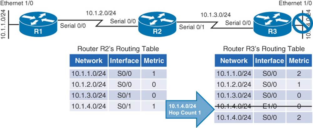
Figure 1-6 Routing Loop: After Link Failure
The problem with this scenario is that the 10.1.4.0 /24 entry in Router R2’s routing table was because of an advertisement that Router R2 received from Router R3. Now, Router R3 is relying on that route, which is no longer valid. The routing loop continues as Router R3 advertises its newly learned route of 10.1.4.0 /24 with a metric of 2 to its neighbor, Router R2. Because Router R2 originally learned the 10.1.4.0 /24 network from Router R3, when it sees Router R3 advertising that same route with a metric of 2, the network gets updated in Router R2’s routing table to have a metric of 3, as shown in Figure 1-7.
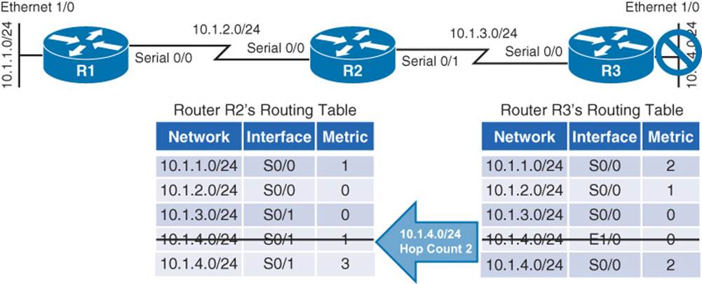
Figure 1-7 Routing Loop: Routers R2 and R3 Incrementing the Metric for 10.1.4.0 /24
The metric for the 10.1.4.0 /24 network continues to increment in the routing tables for both Routers R2 and R3, until the metric reaches a value considered to be an unreachable value (for example, 16 in the case of RIP). This process is referred to as a routing loop.
Distance-vector routing protocols typically use one of two approaches for preventing routing loops:
![]() Split Horizon: The Split Horizon feature prevents a route learned on one interface from being advertised back out of that same interface.
Split Horizon: The Split Horizon feature prevents a route learned on one interface from being advertised back out of that same interface.
![]() Poison Reverse: The Poison Reverse feature causes a route received on one interface to be advertised back out of that same interface with a metric considered to be infinite.
Poison Reverse: The Poison Reverse feature causes a route received on one interface to be advertised back out of that same interface with a metric considered to be infinite.
Having either approach applied to the previous example would have prevented Router R3 from adding the 10.1.4.0 /24 network into its routing table based on an advertisement from Router R2.
Routing protocols falling under the distance-vector category include
![]() Routing Information Protocol (RIP): A distance-vector routing protocol that uses a metric of hop count. The maximum number of hops between two routers in an RIP-based network is 15. Therefore, a hop count of 16 is considered to be infinite. Also, RIP is an IGP. Three primary versions of RIP exist. RIPv1 periodically broadcasts its entire IP routing table, and it supports only fixed-length subnet masks. RIPv2 supports variable-length subnet masks, and it uses multicasts (to a multicast address of 224.0.0.9) to advertise its IP routing table, as opposed to broadcasts. RIP next generation (RIPng) supports the routing of IPv6 networks, while RIPv1 and RIPv2 support the routing of IPv4 networks.
Routing Information Protocol (RIP): A distance-vector routing protocol that uses a metric of hop count. The maximum number of hops between two routers in an RIP-based network is 15. Therefore, a hop count of 16 is considered to be infinite. Also, RIP is an IGP. Three primary versions of RIP exist. RIPv1 periodically broadcasts its entire IP routing table, and it supports only fixed-length subnet masks. RIPv2 supports variable-length subnet masks, and it uses multicasts (to a multicast address of 224.0.0.9) to advertise its IP routing table, as opposed to broadcasts. RIP next generation (RIPng) supports the routing of IPv6 networks, while RIPv1 and RIPv2 support the routing of IPv4 networks.
![]() Enhanced Interior Gateway Routing Protocol (EIGRP): A Cisco-proprietary protocol until early 2013, EIGRP has been popular in Cisco-only networks; however, other vendors can now implement EIGRP on their routers.
Enhanced Interior Gateway Routing Protocol (EIGRP): A Cisco-proprietary protocol until early 2013, EIGRP has been popular in Cisco-only networks; however, other vendors can now implement EIGRP on their routers.
EIGRP is classified as an advanced distance-vector routing protocol, because it improves on the fundamental characteristics of a distance-vector routing protocol. For example, EIGRP does not periodically send out its entire IP routing table to its neighbors. Instead it uses triggered updates, and it converges quickly. Also, EIGRP can support multiple routed protocols (for example, IPv4 and IPv6). EIGRP can even advertise network services (for example, route plan information for a unified communications network) using the Cisco Service Advertisement Framework (SAF).
By default, EIGRP uses bandwidth and delay in its metric calculation; however, other parameters can be considered. These optional parameters include reliability, load, and maximum transmission unit (MTU) size.
The algorithm EIGRP uses for its route selection is not Dijkstra’s Shortest Path First algorithm (as used by OSPF). Instead, EIGRP uses Diffusing Update Algorithm (DUAL).
Link-State
Rather than having neighboring routers exchange their full routing tables with one another, a link-state routing protocol allows routers to build a topological map of a network. Then, similar to a global positioning system (GPS) in a car, a router can execute an algorithm to calculate an optimal path (or paths) to a destination network.
Routers send link-state advertisements (LSA) to advertise the networks they know how to reach. Routers then use those LSAs to construct the topological map of a network. The algorithm run against this topological map is Dijkstra’s Shortest Path First algorithm.
Unlike distance-vector routing protocols, link-state routing protocols exchange full routing information only when two routers initially form their adjacency. Then, routing updates are sent in response to changes in the network, as opposed to being sent periodically. Also, link-state routing protocols benefit from shorter convergence times, as compared to distance-vector routing protocols (although convergence times are comparable to EIGRP).
Routing protocols that can be categorized as link-state routing protocols include
![]() Open Shortest Path First (OSPF): A link-state routing protocol that uses a metric of cost, which is based on the link speed between two routers. OSPF is a popular IGP, because of its scalability, fast convergence, and vendor interoperability.
Open Shortest Path First (OSPF): A link-state routing protocol that uses a metric of cost, which is based on the link speed between two routers. OSPF is a popular IGP, because of its scalability, fast convergence, and vendor interoperability.
![]() Intermediate System–to–Intermediate System (IS-IS): This link-state routing protocol is similar in its operation to OSPF. It uses a configurable, yet dimensionless, metric associated with an interface and runs Dijkstra’s Shortest Path First algorithm. Although using IS-IS as an IGP offers the scalability, fast convergence, and vendor interoperability benefits of OSPF, it has not been as widely deployed as OSPF.
Intermediate System–to–Intermediate System (IS-IS): This link-state routing protocol is similar in its operation to OSPF. It uses a configurable, yet dimensionless, metric associated with an interface and runs Dijkstra’s Shortest Path First algorithm. Although using IS-IS as an IGP offers the scalability, fast convergence, and vendor interoperability benefits of OSPF, it has not been as widely deployed as OSPF.
Path-Vector
A path-vector routing protocol includes information about the exact path packets take to reach a specific destination network. This path information typically consists of a series of autonomous systems through which packets travel to reach their destination. Border Gateway Protocol (BGP) is the only path-vector protocol you are likely to encounter in a modern network.
Also, BGP is the only EGP in widespread use today. In fact, BGP is considered to be the routing protocol that runs the Internet, which is an interconnection of multiple autonomous systems.
BGP’s path selection is not solely based on AS hops, however. BGP has a variety of other parameters that it can consider. Interestingly, none of those parameters are based on link speed. Also, although BGP is incredibly scalable, it does not quickly converge in the event of a topological change. The current version of BGP is BGP version 4 (BGP-4). However, an enhancement to BGP-4, called Multiprotocol BGP (MP-BGP), supports the routing of multiple routed protocols, such as IPv4 and IPv6.
Summary of Categories
As a reference, Table 1-2 categorizes the previously listed routing protocols, based on their type and whether they are primarily an IGP or an EGP.
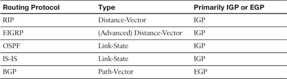
Table 1-2 Routing Protocol Characteristics
Note that a network can simultaneously support more than one routing protocol through the process of route redistribution. For example, a router could have one of its interfaces participating in an OSPF area of the network and have another interface participating in an EIGRP area of the network. This router could then take routes learned through OSPF and inject those routes into the EIGRP routing process. Similarly, EIGRP-learned routes could be redistributed into the OSPF routing process.
Network Technology Fundamentals
When designing a new network or analyzing an existing network, the ability to determine how traffic flows through that network is a necessary skill. Traffic flow is determined both by the traffic type (for example, unicast, multicast, broadcast, or anycast) and the network architecture type (for example, point-to-point, broadcast, and nonbroadcast multiaccess [NMBA]). This section provides you with the basic characteristics of these network technologies.
Network Traffic Types
Traffic can be sent to a single network host, all hosts on a subnet, or a select grouping of hosts that requested to receive the traffic. These traffic types include unicast, broadcast, multicast, and anycast.
Older routing protocols, such as RIPv1 and IGRP (the now-antiquated predecessor to EIGRP), used broadcasts to advertise routing information; however, most modern IGPs use multicasts for their route advertisements.
Note
BGP establishes a TCP session between peers. Therefore, unicast transmissions are used for BGP route advertisement.
Unicast
Most network traffic is unicast in nature, meaning that traffic travels from a single source device to a single destination device. Figure 1-8 illustrates an example of a unicast transmission. In IPv4 networks, unicast addresses are made up of Class A, B, and C addresses. IPv6 networks instead use global unicast addresses, which begin with the 2000::/3 prefix.
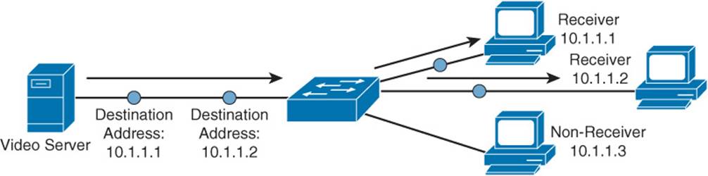
Figure 1-8 Sample IPv4 Unicast Transmission
Broadcast
Broadcast traffic travels from a single source to all destinations in a subnet (that is, a broadcast domain). A broadcast address of 255.255.255.255 might seem that it would reach all hosts on an interconnected network. However, 255.255.255.255 targets all devices on a single network, specifically the network local to the device sending a packet destined for 255.255.255.255. Another type of broadcast address is a directed broadcast address, which targets all devices in a remote network. For example, the address 172.16.255.255 /16 is a directed broadcast targeting all devices in the 172.16.0.0 /16 network. Figure 1-9 illustrates an example of a broadcast transmission.
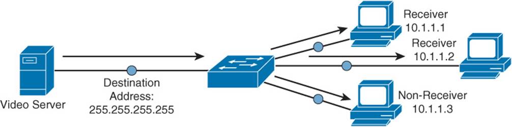
Figure 1-9 Sample IPv4 Broadcast Transmission
Note
Broadcasts are used in IPv4 networks, but not in IPv6 networks.
Multicast
Multicast technology provides an efficient mechanism for a single host to send traffic to multiple, yet specific, destinations. For example, imagine a network with 100 users. Twenty of those users want to receive a video stream from a video server. With a unicast solution, the video server would have to send 20 individual streams, one stream for each recipient. Such a solution could consume a significant amount of network bandwidth and put a heavy processor burden on the video server.
With a broadcast solution, the video server would only have to send the video stream once; however, the stream would be received by every device on the local subnet, even devices not wanting to receive it. Even though those devices do not want to receive the video stream, they still have to pause what they are doing and take time to check each of these unwanted packets.
As shown in Figure 1-10, multicast offers a compromise, allowing the video server to send the video stream only once, and only sending the video stream to devices on the network that want to receive the stream.
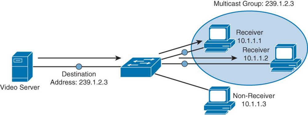
Figure 1-10 Sample IPv4 Multicast Transmission
What makes this possible in IPv4 networks is the use of a Class D address. A Class D address, such as 239.1.2.3, represents the address of a multicast group. The video server could, in this example, send a single copy of each video stream packet destined for 239.1.2.3. Devices wanting to receive the video stream can join the multicast group. Based on the device request, switches and routers in the topology can then dynamically determine out of which ports the video stream should be forwarded.
Note
In IPv6 networks, multicast addresses have a prefix of ff00::/8.
Anycast
With anycast, a single IPv6 address is assigned to multiple devices, as depicted in Figure 1-11. The communication flow is one-to-nearest (from the perspective of a router’s routing table).
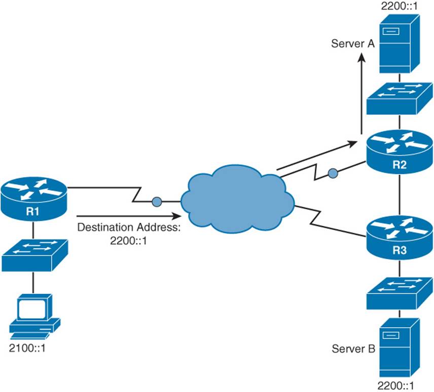
Figure 1-11 IPv6 Anycast Example
In Figure 1-11, a client with an IPv6 address of 2100::1 wants to send traffic to a destination IPv6 address of 2200::1. Notice that two servers (Server A and Server B) have an IPv6 address of 2200::1. In the figure, the traffic destined for 2200::1 is sent to Server A through Router R2, because the network on which Server A resides appears to be closer than the network on which Server B resides, from the perspective of Router R1’s IPv6 routing table.
Note
Anycast is an IPv6 concept and is not found in IPv4 networks. Also, note that IPv6 anycast addresses are not unique from IPv6 unicast addresses.
Network Architecture Types
Another set of network technologies that impact routing, and determine traffic flow, deal with network architecture types (for example, point-to-point, broadcast, and NBMA). For design and troubleshooting purposes, you should be familiar with the characteristics of each.
Point-to-Point Network
A very basic network architecture type is a point-to-point network. As seen in Figure 1-12, a point-to-point network segment consists of a single network link interconnecting two routers. This network type is commonly found on serial links.
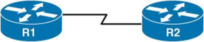
Figure 1-12 Point-to-Point Network Type
Broadcast Network
A broadcast network segment uses an architecture in which a broadcast sent from one of the routers on the network segment is propagated to all other routers on that segment. An Ethernet network, as illustrated in Figure 1-13, is a common example of a broadcast network.
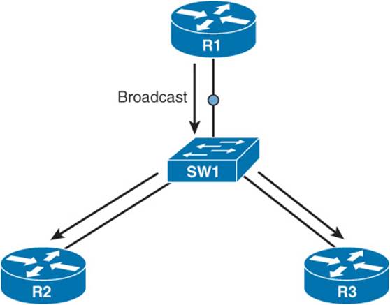
Figure 1-13 Broadcast Network Type
NBMA
As its name suggests, a nonbroadcast multiaccess (NBMA) network does not support broadcasts. As a result, if an interface on a router connects to two other routers, as depicted in Figure 1-14, individual messages must be sent to each router.
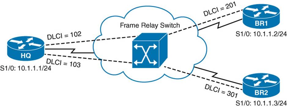
Figure 1-14 NBMA Network Type
The absence of broadcast support also implies an absence of multicast support. This can lead to an issue with dynamic routing protocols (such as OSPF and EIGRP) that dynamically form neighborships with neighboring routers discovered through multicasts. Because neighbors cannot be dynamically discovered, neighboring IP addresses must be statically configured. Examples of NBMA networks include ATM and Frame Relay.
The requirement for static neighbor configuration is not the only routing protocol issue stemming from an NBMA network. Consider the following:

![]() Split Horizon issues: Distance-vector routing protocols (RIP and EIGRP, for example) can use the previously mentioned Split Horizon rule, which prevents routes learned on one interface from being advertised back out of that same interface. Consider Figure 1-14 again. Imagine that Router BR2 advertised a route to Router HQ, and Router HQ had Split Horizon enabled for its S 1/0 interface. That condition would prevent Router HQ from advertising that newly learned route to Router BR1, because it would be advertising that route out the same interface on which it was learned. Fortunately, in situations like this, you can administratively disable Split Horizon.
Split Horizon issues: Distance-vector routing protocols (RIP and EIGRP, for example) can use the previously mentioned Split Horizon rule, which prevents routes learned on one interface from being advertised back out of that same interface. Consider Figure 1-14 again. Imagine that Router BR2 advertised a route to Router HQ, and Router HQ had Split Horizon enabled for its S 1/0 interface. That condition would prevent Router HQ from advertising that newly learned route to Router BR1, because it would be advertising that route out the same interface on which it was learned. Fortunately, in situations like this, you can administratively disable Split Horizon.
![]() Designated router issues: Recall from your CCNA studies that a broadcast network (for example, an Ethernet network) OSPF elects a designated router (DR), with which all other routers on a network segment form an adjacency. Interestingly, OSPF attempts to elect a DR on an NMBA network, by default. Once again considering Figure 1-14, notice that only Router HQ has a direct connection to the other routers; therefore, Router HQ should be the DR. This election might not happen without administrative intervention, however. Specifically, in such a topology, you would need to set the OSPF Priority to 0 on both Routers BR1 and BR2, which prevents them from participating in a DR election.
Designated router issues: Recall from your CCNA studies that a broadcast network (for example, an Ethernet network) OSPF elects a designated router (DR), with which all other routers on a network segment form an adjacency. Interestingly, OSPF attempts to elect a DR on an NMBA network, by default. Once again considering Figure 1-14, notice that only Router HQ has a direct connection to the other routers; therefore, Router HQ should be the DR. This election might not happen without administrative intervention, however. Specifically, in such a topology, you would need to set the OSPF Priority to 0 on both Routers BR1 and BR2, which prevents them from participating in a DR election.
TCP/IP Fundamentals
Recall from your CCNA studies that the Internet layer of the TCP/IP stack maps to Layer 3 (that is, the network layer) of the Open Systems Interconnection (OSI) model. While multiple routed protocols (for example, IP, IPX, and AppleTalk) reside at the OSI model’s network layer, Internet Protocol (IP) has become the de-facto standard for network communication.
Sitting just above IP, at the transport layer (of both the TCP/IP and OSI models) is Transmission Control Protocol (TCP) and User Datagram Protocol (UDP). This section reviews the basic operation of the TCP/IP suite of protocols, as their behavior is the foundation of the routing topics in the remainder of this book.
IP Characteristics
Figure 1-15 shows the IP version 4 packet header format.
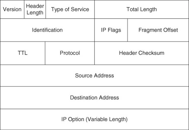
Figure 1-15 IP Version 4 Packet Header Format
The functions of the fields in an IPv4 header are as follows:
![]() Version field: The Version field indicates IPv4 (with a value of 0100).
Version field: The Version field indicates IPv4 (with a value of 0100).
![]() Header Length field: The Header Length field (commonly referred to as the Internet Header Length (IHL) field) is a 4-bit field indicating the number of 4-byte words in the IPv4 header.
Header Length field: The Header Length field (commonly referred to as the Internet Header Length (IHL) field) is a 4-bit field indicating the number of 4-byte words in the IPv4 header.
![]() Type of Service field: The Type of Service (ToS) field (commonly referred to as the ToS Byte or DHCP field) has 8 bits used to set quality of service (QoS) markings. Specifically, the 6 leftmost bits are used for the Differentiated Service Code Point (DSCP) marking, and the 2 rightmost bits are used for Explicit Congestion Notification (an extension of Weighted Random Early Detection (WRED), used for flow control).
Type of Service field: The Type of Service (ToS) field (commonly referred to as the ToS Byte or DHCP field) has 8 bits used to set quality of service (QoS) markings. Specifically, the 6 leftmost bits are used for the Differentiated Service Code Point (DSCP) marking, and the 2 rightmost bits are used for Explicit Congestion Notification (an extension of Weighted Random Early Detection (WRED), used for flow control).
![]() Total Length field: The Total Length field is a 16-bit value indicating the size of the packet (in bytes).
Total Length field: The Total Length field is a 16-bit value indicating the size of the packet (in bytes).
![]() Identification field: The Identification field is a 16-bit value used to mark fragments that came from the same packet.
Identification field: The Identification field is a 16-bit value used to mark fragments that came from the same packet.
![]() IP Flags field: The IP Flags field is a 3-bit field, where the first bit is always set to a 0. The second bit (the Don’t Fragment [DF] bit) indicates that a packet should not be fragmented. The third bit (the More Fragments [MF] bit) is set on all of a packet’s fragments, except the last fragment.
IP Flags field: The IP Flags field is a 3-bit field, where the first bit is always set to a 0. The second bit (the Don’t Fragment [DF] bit) indicates that a packet should not be fragmented. The third bit (the More Fragments [MF] bit) is set on all of a packet’s fragments, except the last fragment.
![]() Fragment Offset field: The Fragment Offset field is a 13-bit field that specifies the offset of a fragment from the beginning of the first fragment in a packet, in 8-byte units.
Fragment Offset field: The Fragment Offset field is a 13-bit field that specifies the offset of a fragment from the beginning of the first fragment in a packet, in 8-byte units.
![]() Time to Live (TTL) field: The Time to Live (TTL) field is an 8-bit field that is decremented by 1 every time the packet is routed from one IP network to another (that is, passes through a router). If the TTL value ever reaches 0, the packet is discarded from the network. This behavior helps prevent routing loops.
Time to Live (TTL) field: The Time to Live (TTL) field is an 8-bit field that is decremented by 1 every time the packet is routed from one IP network to another (that is, passes through a router). If the TTL value ever reaches 0, the packet is discarded from the network. This behavior helps prevent routing loops.
![]() Protocol field: The Protocol field is an 8-bit field that specifies the type of data encapsulated in the packet. TCP and UDP are common protocols identified by this field.
Protocol field: The Protocol field is an 8-bit field that specifies the type of data encapsulated in the packet. TCP and UDP are common protocols identified by this field.
![]() Header Checksum field: The Header Checksum field is a 16-bit field that performs error checking for a packet’s header. Interestingly, this error checking is performed for UDP segments, in addition to TCP segments, even though UDP is itself an “unreliable” protocol.
Header Checksum field: The Header Checksum field is a 16-bit field that performs error checking for a packet’s header. Interestingly, this error checking is performed for UDP segments, in addition to TCP segments, even though UDP is itself an “unreliable” protocol.
![]() Source Address field: The 32-bit Source Address field indicates the source of an IPv4 packet.
Source Address field: The 32-bit Source Address field indicates the source of an IPv4 packet.
![]() Destination Address field: The 32-bit Destination Address field indicates the destination of an IPv4 packet.
Destination Address field: The 32-bit Destination Address field indicates the destination of an IPv4 packet.
![]() IP Option field: The IP Option field is a seldom-used field that can specify a variety of nondefault packet options. If the IP Option field is used, its length varies based on the options specified.
IP Option field: The IP Option field is a seldom-used field that can specify a variety of nondefault packet options. If the IP Option field is used, its length varies based on the options specified.
An IPv6 packet header, as seen in Figure 1-16, is simpler in structure than the IPv4 packet header.
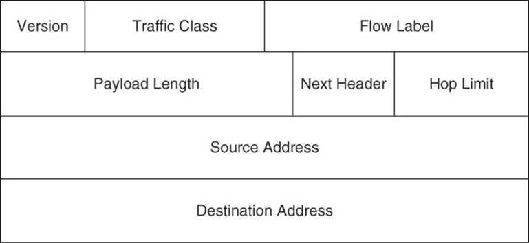
Figure 1-16 IP Version 6 Packet Header Format
The purposes of the fields found in an IPv6 header are as follows:
![]() Version field: Like an IPv4 header, an IPv6 header has a Version field, indicating IPv6 (with a value of 0110).
Version field: Like an IPv4 header, an IPv6 header has a Version field, indicating IPv6 (with a value of 0110).
![]() Traffic Class field: The Traffic Class field is the same size, performs the same functions, and takes on the same values as the Type of Service field in an IPv4 header.
Traffic Class field: The Traffic Class field is the same size, performs the same functions, and takes on the same values as the Type of Service field in an IPv4 header.
![]() Flow Label field: The 20-bit Flow Label field can be used to instruct a router to use a specific outbound connection for a traffic flow (if a router has multiple outbound connections). By having all packets in the same flow use the same connection, the probability of packets arriving at their destination out of order is reduced.
Flow Label field: The 20-bit Flow Label field can be used to instruct a router to use a specific outbound connection for a traffic flow (if a router has multiple outbound connections). By having all packets in the same flow use the same connection, the probability of packets arriving at their destination out of order is reduced.
![]() Payload Length field: The Payload Length field is a 16-bit field indicating the size (in bytes) of the payload being carried by an IPv6 packet.
Payload Length field: The Payload Length field is a 16-bit field indicating the size (in bytes) of the payload being carried by an IPv6 packet.
![]() Next Header field: The Next Header field, similar to the Protocol field in an IPv4 header, indicates the type of header encapsulated in the IPv6 header. Typically, this 8-bit header indicates a specific transport layer protocol.
Next Header field: The Next Header field, similar to the Protocol field in an IPv4 header, indicates the type of header encapsulated in the IPv6 header. Typically, this 8-bit header indicates a specific transport layer protocol.
![]() Hop Limit field: The 8-bit Hop Limit field replaces, and performs the same function as, the IPv4 header’s TTL field. Specifically, it is decremented at each router hop until it reaches 0, at which point the packet is discarded.
Hop Limit field: The 8-bit Hop Limit field replaces, and performs the same function as, the IPv4 header’s TTL field. Specifically, it is decremented at each router hop until it reaches 0, at which point the packet is discarded.
![]() Source Address field: Similar to the IPv4 header’s 32-bit Source Address field, the IPv6 Source Address field is 128 bits in size and indicates the source of an IPv6 packet.
Source Address field: Similar to the IPv4 header’s 32-bit Source Address field, the IPv6 Source Address field is 128 bits in size and indicates the source of an IPv6 packet.
![]() Destination Address field: Similar to the IPv4 header’s 32-bit Destination Address field, the IPv6 Destination Address field is 128 bits in size and indicates the destination of an IPv6 packet.
Destination Address field: Similar to the IPv4 header’s 32-bit Destination Address field, the IPv6 Destination Address field is 128 bits in size and indicates the destination of an IPv6 packet.
Routing Review
As a review from your CCNA studies, recall how the fields in an IP header are used to route a packet from one network to another. While the process is similar for IPv6, the following example considers IPv4.
In the topology shown in Figure 1-17, PC1 needs to send traffic to Server1. Notice that these devices are on different networks. So, the question becomes, “How does a packet from a source IP address of 192.168.1.2 get forwarded to a destination IP address of 192.168.3.2?”
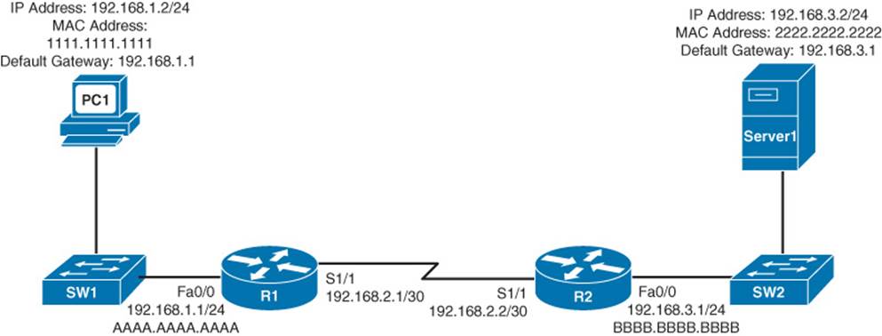
Figure 1-17 Basic Routing Topology
The answer is routing, as summarized in the following steps:
Step 1. PC1 compares its IP address and subnet mask of 192.168.1.2 /24 with the destination IP address and subnet mask of 192.168.3.2 /24. PC1 concludes that the destination IP address resides on a remote subnet. Therefore, PC1 needs to send the packet to its default gateway, which could have been manually configured on PC1 or dynamically learned through Dynamic Host Configuration Protocol (DHCP). In this example, PC1 has a default gateway of 192.168.1.1 (Router R1). However, to construct a Layer 2 frame, PC1 also needs the MAC address of its default gateway. PC1 sends an Address Resolution Protocol (ARP) request for Router R1’s MAC address. After PC1 receives an ARP reply from Router R1, PC1 adds Router R1’s MAC address to its ARP cache. PC1 now sends its data in a frame destined for Server1, as shown in Figure 1-18.
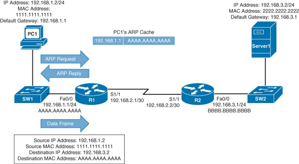
Figure 1-18 Basic Routing: Step 1
Note
ARP uses broadcasts, which are not supported by IPv6. Therefore, IPv6 exchanges Neighbor Discovery messages with adjacent devices to perform functions similar to ARP.
Step 2. Router R1 receives the frame sent from PC1 and interrogates the IP header. An IP header contains a Time to Live (TTL) field, which is decremented once for each router hop. Therefore, Router R1 decrements the packet’s TTL field. If the value in the TTL field is reduced to 0, the router discards the frame and sends a time exceeded Internet Control Message Protocol (ICMP) message back to the source. Assuming that the TTL is not decremented to 0, Router R1 checks its routing table to determine the best path to reach network 192.168.3.0 /24. In this example, Router R1’s routing table has an entry stating that network 192.168.3.0 /24 is accessible through interface Serial 1/1. Note that ARPs are not required for serial interfaces, because these interface types do not have MAC addresses. Router R1, therefore, forwards the frame out of its Serial 1/1 interface, as shown in Figure 1-19.
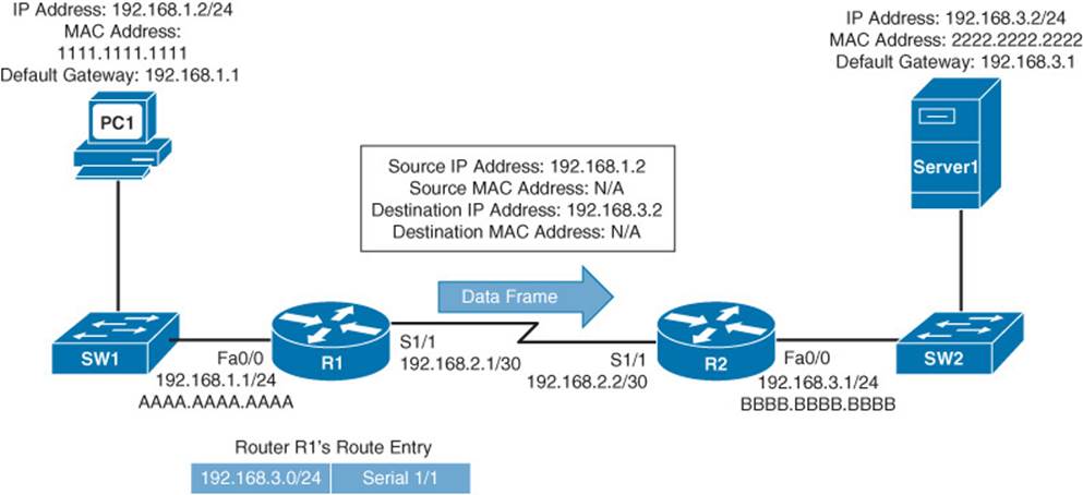
Figure 1-19 Basic Routing: Step 2
Step 3. When Router R2 receives the frame, it decrements the TTL in the IP header, just as Router R1 did. Again, assuming that the TTL did not get decremented to 0, Router R2 interrogates the IP header to determine the destination network. In this case, the destination network of 192.168.3.0 /24 is directly attached to Router R2’s Fast Ethernet 0/0 interface. Similar to how PC1 sent out an ARP request to determine the MAC address of its default gateway, Router R2 sends an ARP request to determine the MAC address of Server1. After an ARP Reply is received from Server1, Router R2 forwards the frame out of its Fast Ethernet 0/0 interface to Server1, as illustrated in Figure 1-20.
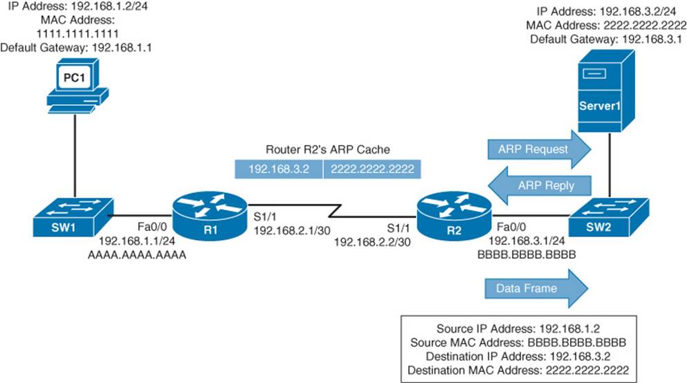
Figure 1-20 Basic Routing: Step 3
Asymmetric Routing
Many times, routing operations are impacted by Layer 2 switching in a network. As an example, consider a situation, as depicted in Figure 1-21, where a VLAN is spread across multiple access layer switches, and a First-Hop Redundancy Protocol (FHRP) (for example, HSRP, VRRP, or GLBP) is being used on multilayer switches at the distribution layer.
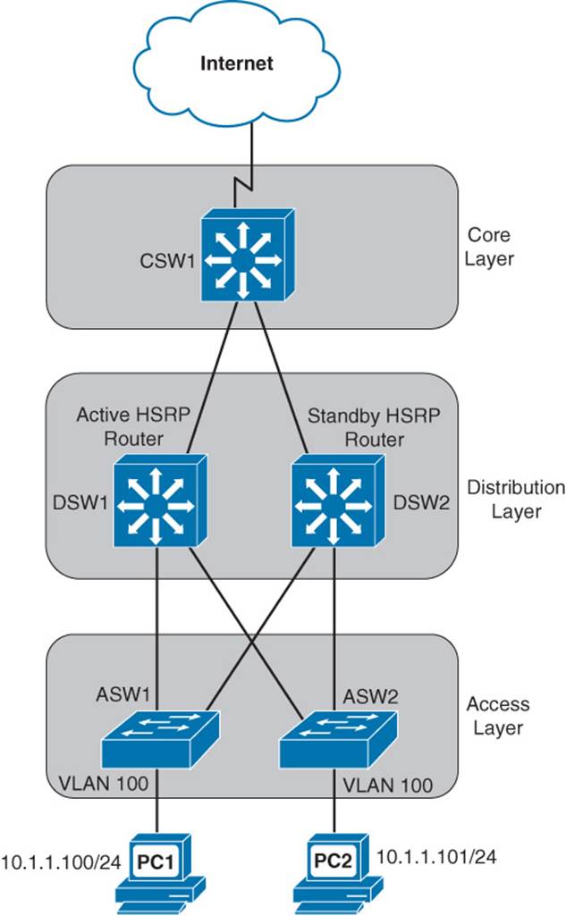
Figure 1-21 Topology with Asymmetric Routing
In the figure, notice that VLAN 100 (that is, 10.1.1.0 /24) exists on both switches ASW1 and ASW2 at the access layer. Also, notice that there are two multilayer switches (that is, DSW1 and DSW2) at the distribution layer with an HSRP configuration to provide default gateway redundancy to hosts in VLAN 100. The multilayer switch in the core layer (that is, CSW1) supports equal-cost load balancing between DSW1 and DSW2.
Focusing on the HSRP configuration, imagine that DSW1 is the active HSRP “router” and DSW2 is the standby HSRP “router.” Next, imagine that PC1 sends traffic out to the Internet. The traffic flows through ASW1, DSW1 (the active HSRP router), and CSW1, as shown in Figure 1-22.
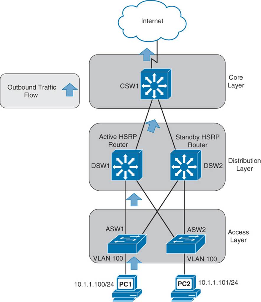
Figure 1-22 Unidirectional Outbound Traffic
A challenge with this common scenario can occur with the return traffic, as illustrated in Figure 1-23. The return traffic flows from the Internet and into CSW1, which then load-balances between DSW1 and DSW2. When the path through DSW1 is used, the MAC address of PC1 is known to DSW1’s ARP cache (because it just saw PC1’s MAC address being used as the source MAC address in a packet going out to the Internet). However, when the path through DSW2 is used, DSW2 might not have PC1’s MAC address in its ARP cache (because PC1 isn’t normally using DSW2 as its default gateway). As a result, DSW2 floods this unknown unicast traffic out all its other ports. This issue is known as asymmetric routing, because traffic might leave through one path (for example, through DSW1) and return through a different path (for example, through DSW2). Another name given to this issue is unicast flooding, because of the potential for a backup FHRP router or multilayer switch to flood unknown unicast traffic for returning traffic.
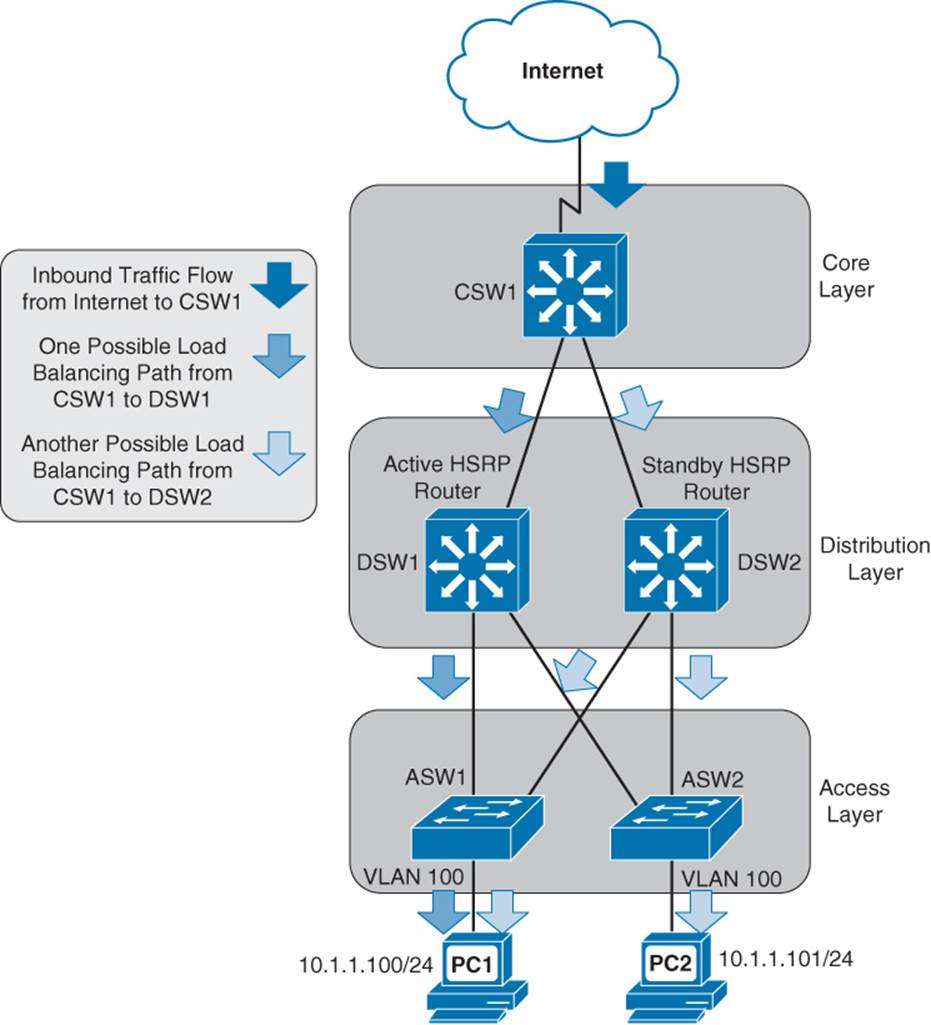
Figure 1-23 Unidirectional Flooding of Inbound Traffic
Cisco recommends that you do not span a VLAN across more than one access layer switch to avoid such an issue. However, if a particular design requires the spanning of a VLAN across multiple access layer switches, the best-practice recommendation from Cisco is that you adjust the FHRP device’s ARP timer to be equal to or less than the Content Addressable Memory (CAM) aging time. Otherwise, the CAM table entry for the end station will time out before the ARP entry times out, meaning that the FHRP device knows (from its ARP cache) the MAC address corresponding to the destination IP address, and therefore does not need to ARP for the MAC address. However, if the CAM entry has timed out, the FHRP device needs to flood the traffic to make sure that it gets to the intended destination. With an ARP timer equal to or less than the CAM aging time, there will never be an ARP entry for a MAC address not also stored in the CAM table. As a result, if the FHRP device’s ARP entry has timed out, it will use ARP to get the MAC address of the destination IP address, thus causing the CAM table to learn the appropriate egress port.
Maximum Transmission Unit
A Maximum Transmission Unit (MTU), in the context of Cisco routers, typically refers to the largest packet size supported on a router interface; 1500 bytes is a common value. Smaller MTU sizes result in more overhead, because more packets (and therefore more headers) are required to transmit the same amount of data. However, if you are sending data over slower link speeds, large MTU values could cause delay for latency-sensitive traffic.
Note
Latency is the time required for a packet to travel from its source to destination. Some applications, such as Voice over IP (VoIP), are latency sensitive, meaning that they do not perform satisfactorily if the latency of their packets is too high. For example, the G.114 recommendation states that the one-way latency for VoIP traffic should not exceed 150 ms.Latency is a factor in the calculation of the bandwidth-delay product. Specifically, the bandwidth-delay product is a measurement of the maximum number of bits that can be on a network segment at any one time, and it is calculated by multiplying the segment’s bandwidth (in bits/sec) by the latency packets experience as they cross the segment (in sec). For example, a network segment with a bandwidth of 768 kbps and an end-to-end latency of 100 ms would have a bandwidth-delay product of 76,800 bits (that is 768,000 * 0.1 = 76,800).
ICMP Messages
Another protocol residing alongside IP at Layer 3 of the OSI model is Internet Control Message Protocol (ICMP). ICMP is most often associated with the Ping utility, used to check connectivity with a remote network address (using ICMP Echo Request and ICMP Echo Reply messages).
Note
There is some debate in the industry about where ICMP fits into the OSI model. Although it is generally considered to be a Layer 3 protocol, be aware that ICMP is encapsulated inside of an IP packet, and some of its messages are based on Layer 4 events.
ICMP does have other roles beyond Ping. By using a variety of message types, ICMP can be used by network devices (for example, routers) to provide information to one another. Figure 1-24 shows the structure of an ICMP packet header.
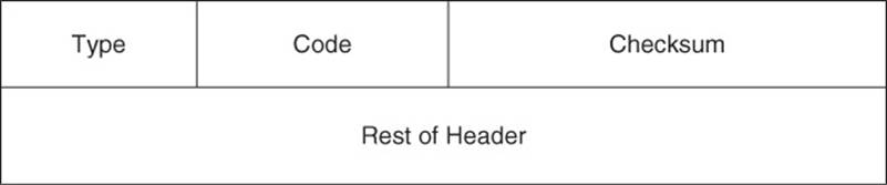
Figure 1-24 ICMP Packet Header Format
The purposes of the fields found in an ICMP packet header are as follows:
![]() Type: The 1-byte Type field contains a number indicating the specific type of ICMP message. Here are a few examples: A Type 0 is an Echo Reply message, a Type 3 is a Destination Unreachable message, a Type 5 is a Redirect message, and a Type 8 is an ICMP Echo Requestmessage.
Type: The 1-byte Type field contains a number indicating the specific type of ICMP message. Here are a few examples: A Type 0 is an Echo Reply message, a Type 3 is a Destination Unreachable message, a Type 5 is a Redirect message, and a Type 8 is an ICMP Echo Requestmessage.
![]() Code: The 1-byte Code field further defines the ICMP type. For example, there are 16 codes for Destination Unreachable ICMP messages. Here are a couple of examples: A code of 0 means that the destination network is unreachable, while a code of 1 means that the destination host is unreachable.
Code: The 1-byte Code field further defines the ICMP type. For example, there are 16 codes for Destination Unreachable ICMP messages. Here are a couple of examples: A code of 0 means that the destination network is unreachable, while a code of 1 means that the destination host is unreachable.
![]() Checksum: The 2-byte Checksum field performs error checking.
Checksum: The 2-byte Checksum field performs error checking.
![]() Rest of Header: The 4-byte Rest of Header field is 4 bytes in length, and its contents are dependent on the specific ICMP type.
Rest of Header: The 4-byte Rest of Header field is 4 bytes in length, and its contents are dependent on the specific ICMP type.
While ICMP has multiple messages types and codes, for purposes of the ROUTE exam, you should primarily be familiar with the two following ICMP message types:
![]() Destination Unreachable: If a packet enters a router destined for an address that the router does not know how to reach, the router can let the sender know by sending a Destination Unreachable ICMP message back to the sender.
Destination Unreachable: If a packet enters a router destined for an address that the router does not know how to reach, the router can let the sender know by sending a Destination Unreachable ICMP message back to the sender.
![]() Redirect: A host might have routing information indicating that to reach a particular destination network, packets should be sent to a certain next-hop IP address. However, if network conditions change and a different next-hop IP address should be used, the original next-hop router can let the host know to use a different path by sending the host a Redirect ICMP message.
Redirect: A host might have routing information indicating that to reach a particular destination network, packets should be sent to a certain next-hop IP address. However, if network conditions change and a different next-hop IP address should be used, the original next-hop router can let the host know to use a different path by sending the host a Redirect ICMP message.
TCP Characteristics
TCP is commonly touted as being a reliable transport mechanism, as compared to its unreliable counterpart, UDP. Examination of the TCP segment header format, as shown in Figure 1-25, provides valuable insight into how this reliability happens.
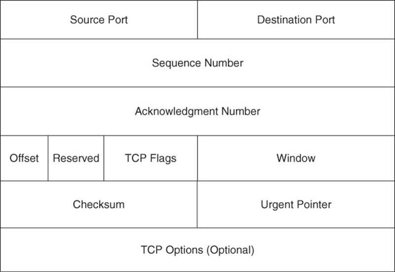
Figure 1-25 TCP Segment Header Format
The purposes of the fields found in a TCP segment header are as follows:
![]() Source Port field: The Source Port field is a 16-bit field indicating the sending port number.
Source Port field: The Source Port field is a 16-bit field indicating the sending port number.
![]() Destination Port field: The Destination Port field is a 16-bit field indicating the receiving port number.
Destination Port field: The Destination Port field is a 16-bit field indicating the receiving port number.
![]() Sequence Number field: The Sequence Number field is a 32-bit field indicting the amount of data sent during a TCP session. The sending party can be assured that the receiving party really received the data, because the receiving party uses the sequence number as the basis for the acknowledgment number in the next segment it sends back to the sender. Specifically, the acknowledgment number in that segment equals the received sequence number plus 1. Interestingly, at the beginning of a TCP session, the initial sequence number can be any number in the range 0–4,294,967,295 (that is, the range of numbers that can be represented by 32 bits). However, when you are doing troubleshooting and performing a packet capture of a TCP session, the initial sequence number might appear to be a relative sequence number of 0. The use of a relative sequence number can often make data easier to interpret while troubleshooting.
Sequence Number field: The Sequence Number field is a 32-bit field indicting the amount of data sent during a TCP session. The sending party can be assured that the receiving party really received the data, because the receiving party uses the sequence number as the basis for the acknowledgment number in the next segment it sends back to the sender. Specifically, the acknowledgment number in that segment equals the received sequence number plus 1. Interestingly, at the beginning of a TCP session, the initial sequence number can be any number in the range 0–4,294,967,295 (that is, the range of numbers that can be represented by 32 bits). However, when you are doing troubleshooting and performing a packet capture of a TCP session, the initial sequence number might appear to be a relative sequence number of 0. The use of a relative sequence number can often make data easier to interpret while troubleshooting.
![]() Acknowledgment Number field: The 32-bit Acknowledgment Number field is used by the recipient of a segment to request the next segment in the TCP session. The value of this field is calculated by adding 1 to the previously received sequence number.
Acknowledgment Number field: The 32-bit Acknowledgment Number field is used by the recipient of a segment to request the next segment in the TCP session. The value of this field is calculated by adding 1 to the previously received sequence number.
![]() Offset field: The Offset field is a 4-bit field that specifies the offset between the data in a TCP segment and the start of the segment, in units of 4-byte words.
Offset field: The Offset field is a 4-bit field that specifies the offset between the data in a TCP segment and the start of the segment, in units of 4-byte words.
![]() Reserved field: The 3-bit Reserved field is not used, and each of the 3 bits are set to a value of 0.
Reserved field: The 3-bit Reserved field is not used, and each of the 3 bits are set to a value of 0.
![]() TCP Flags field: The TCP Flags field is comprised of 9 flag bits (also known as control bits), which indicate a variety of segment parameters.
TCP Flags field: The TCP Flags field is comprised of 9 flag bits (also known as control bits), which indicate a variety of segment parameters.
![]() Window field: The 16-bit Window field specifies the number of bytes a sender is willing to transmit before receiving an acknowledgment from the receiver.
Window field: The 16-bit Window field specifies the number of bytes a sender is willing to transmit before receiving an acknowledgment from the receiver.
![]() Checksum field: The Checksum field is a 16-bit field that performs error checking for a segment.
Checksum field: The Checksum field is a 16-bit field that performs error checking for a segment.
![]() Urgent Pointer field: The 16-bit Urgent Pointer field indicates that last byte of a segment’s data that was considered urgent. The field specifies the number of bytes between the current sequence number and that urgent data byte.
Urgent Pointer field: The 16-bit Urgent Pointer field indicates that last byte of a segment’s data that was considered urgent. The field specifies the number of bytes between the current sequence number and that urgent data byte.
![]() TCP Options field: The optional TCP Options field can range in size from 0 to 320 bits (as long as the number of bits is evenly divisible by 32), and the field can contain a variety of TCP segment parameters.
TCP Options field: The optional TCP Options field can range in size from 0 to 320 bits (as long as the number of bits is evenly divisible by 32), and the field can contain a variety of TCP segment parameters.
Three-Way Handshake
The process of setting up a TCP session involves a three-way handshake, as listed in the following steps and as illustrated in Figure 1-26.
Step 1. The session initiator sends a Synchronization (SYN) message to the target host.
Step 2. The target host acknowledges receipt of the SYN message with an Acknowledgment (ACK) message and also sends a SYN message of its own.
Step 3. The session initiator receives the SYN messages from the target host and acknowledges receipt by sending an ACK message.
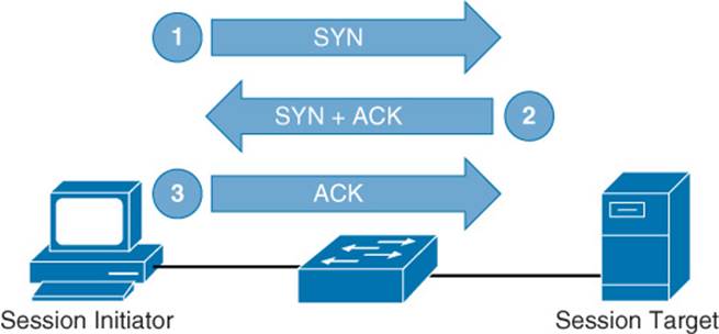
Figure 1-26 TCP Three-Way Handshake
TCP Sliding Window
TCP communication uses windowing, meaning that one or more segments are sent at one time, and a receiver can acknowledge the receipt of all the segments in a window with a single acknowledgment. In some cases, as illustrated in Figure 1-27, TCP uses a sliding window, where the window size begins with one segment. If there is a successful acknowledgment of that one segment (that is, the receiver sends an ACK asking for the next segment), the window size doubles to two segments. Upon successful receipt of those two segments, the next window contains four segments. This exponential increase in window size continues until the receiver does not acknowledge successful receipt of all segments within a certain time period (known as the round-trip time [RTT], which is sometimes called real transfer time), or until a configured maximum window size is reached.
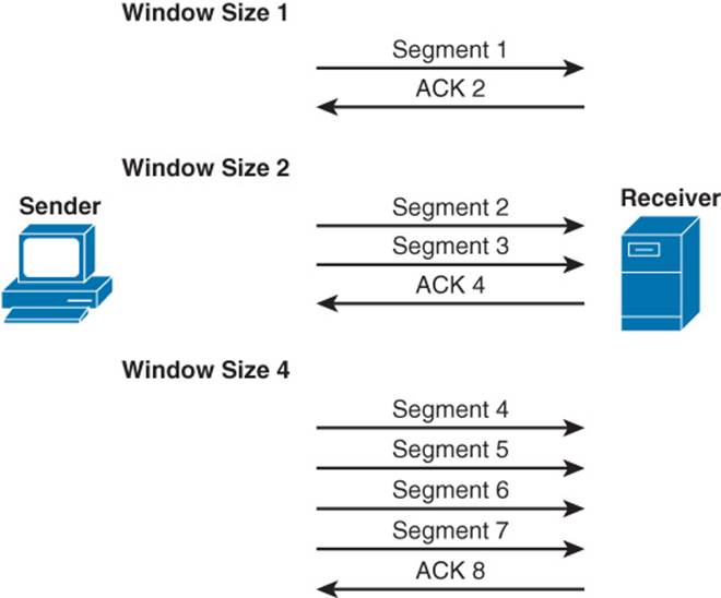
Figure 1-27 TCP Sliding Window
The TCP Maximum Segment Size (MSS) is the amount of data that can be contained in a single TCP segment. The value is dependent on the current TCP window size.
Note
The term Maximum Segment Size (MSS) seems to imply the size of the entire Layer 4 segment (that is, including Layer 2, Layer 3, and Layer 4 headers). However, MSS only refers to the amount of data in a segment.
If a single TCP flow drops a packet, that flow might experience TCP slow start, meaning that the window size is reduced to one segment. The window size then grows exponentially until it reaches one-half of its congestion window size (that is, the window size when congestion was previously experienced). At that point, the window size begins to grow linearly instead of exponentially.
If a router interface’s output queue fills to capacity, all TCP flows can simultaneously start to drop packets, causing all TCP flows to experience slow start. This condition, called global synchronization or TCP synchronization, results in a very inefficient use of bandwidth, because of all TCP flows having reduced window sizes and therefore spending more time waiting for acknowledgments.
Note
To prevent global synchronization, Cisco IOS supports a feature called Weighted Random Early Detection (WRED), which can pseudo-randomly drop packets from flows based on the number of packets currently in a queue and the quality of service (QoS) markings on the packets. By dropping packets before the queue fills to capacity, the global synchronization issue is avoided.
Out-of-Order Delivery
In many routed environments, a router has more than one egress interface that can reach a destination IP address. If load balancing is enabled in such a scenario, some packets in a traffic flow might go out one interface, while other packets go out of another interface. With traffic flowing out of multiple interfaces, there is a chance that the packets will arrive out of order. Fortunately, TCP can help prevent out-of-order packets by either sequencing them in the correct order or by requesting the retransmission of out-of-order packets.
UDP Characteristics
Figure 1-28 presents the structure of a UDP segment header. Because UDP is considered to be a connectionless, unreliable protocol, it lacks the sequence numbering, window size, and acknowledgment numbering present in the header of a TCP segment. Rather the UDP segment’s header contains only source and destination port numbers, a UDP checksum (which is an optional field used to detect transmission errors), and the segment length (measured in bytes).
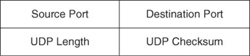
Figure 1-28 UDP Segment Header Format
Because a UDP segment header is so much smaller than a TCP segment header, UDP becomes a good candidate for the transport layer protocol serving applications that need to maximize bandwidth and do not require acknowledgments (for example, audio or video streams). In fact, the primary protocol used to carry voice and video traffic, Real-time Transport Protocol (RTP), is a Layer 4 protocol that is encapsulated inside of UDP.
If RTP is carrying interactive voice or video streams, the latency between the participants in a voice and/or video call should ideally be no greater than 150 ms. To help ensure that RTP experiences minimal latency, even during times of congestion, Cisco recommends a queuing technology called Low Latency Queuing (LLQ). LLQ allows one or more traffic types to be buffered in a priority queue, which is serviced first (up to a maximum bandwidth limit) during times of congestion. Metaphorically, LLQ works much like a carpool lane found in highway systems in larger cities. With a carpool lane, if you are a special type of traffic (for example, a vehicle with two or more passengers), you get to drive in a separate lane with less congestion. However, the carpool lane is not the autobahn (a German highway without a speed limit). You are still restricted as to how fast you can go.
With LLQ, you can treat special traffic types (for example, voice and video using RTP) in a special way, by placing them in a priority queue. Traffic in the priority queue (much like a carpool lane) gets to go ahead of nonpriority traffic; however, there is a bandwidth limit (much like a speed limit) that traffic in the priority queue cannot exceed. Therefore, priority traffic does not starve out nonpriority traffic.
Network Migration Strategies
As networks undergo expansion or as new technologies are introduced, network engineers need to understand the implications of the changes being made. This section identifies a few key areas where change is likely to occur (if it has not already occurred) in enterprise networks.
Routing Protocol Changes
The primary focus of this book is on routing protocols. As you read through the subsequent chapters covering protocols such as RIPng, OSPF, EIGRP, and BGP, be on the lookout for protocol-specific parameters that need to match between neighboring devices.
As one example, in Chapter 4, “Fundamental EIGRP Concepts,” you will read about EIGRP K-values and how they must match between EIGRP neighbors. Therefore, if you make a K-value change on one router, that change needs to be reflected on neighboring routers.
In addition to making adjustments to existing routing protocols, network engineers sometimes need to migrate to an entirely new routing protocol. For example, a network that was running RIP might migrate to OSPF. Two common approaches to routing protocol migration are as follows:
![]() Using Administrative Distance (AD): When migrating from one routing protocol to another, one approach is to configure both routing protocols on all your routers, allowing them to run concurrently. However, when you do your configuration of the new routing protocol, you should make sure that it has a higher AD than the existing routing protocol. This approach allows you to make sure that the new routing protocol has successfully learned all the routes it needs to learn and has appropriate next hops for its route entries. After you are convinced that the new routing protocol is configured appropriately, you can adjust the AD on either the old or the new routing protocol such that the new routing protocol is preferred.
Using Administrative Distance (AD): When migrating from one routing protocol to another, one approach is to configure both routing protocols on all your routers, allowing them to run concurrently. However, when you do your configuration of the new routing protocol, you should make sure that it has a higher AD than the existing routing protocol. This approach allows you to make sure that the new routing protocol has successfully learned all the routes it needs to learn and has appropriate next hops for its route entries. After you are convinced that the new routing protocol is configured appropriately, you can adjust the AD on either the old or the new routing protocol such that the new routing protocol is preferred.
![]() Using route redistribution: Another approach to migrating between routing protocols is to use redistribution, such that you cut over one section of your network at a time, and mutually redistribute routes between portions of your network using the old routing protocol and portions using the new routing protocol. This approach allows you to, at your own pace, roll out and test the new routing protocol in your network locations.
Using route redistribution: Another approach to migrating between routing protocols is to use redistribution, such that you cut over one section of your network at a time, and mutually redistribute routes between portions of your network using the old routing protocol and portions using the new routing protocol. This approach allows you to, at your own pace, roll out and test the new routing protocol in your network locations.
IPv6 Migration
You could argue that there are two kinds of IP networks: those that have already migrated to IPv6 and those that will migrate to IPv6. With the depletion of the IPv4 address space, the adoption of IPv6 for most every IP-based network is an eventuality. Following are a few strategies to consider when migrating your network, or your customers’ networks, from IPv4 to IPv6:
![]() Check equipment for IPv6 compatibility: Before rolling out IPv6, you should check your existing network devices (for example, switches, routers, and firewalls) for IPv6 compatibility. In some cases, you might be able to upgrade the Cisco IOS on your existing gear to add IPv6 support for those devices.
Check equipment for IPv6 compatibility: Before rolling out IPv6, you should check your existing network devices (for example, switches, routers, and firewalls) for IPv6 compatibility. In some cases, you might be able to upgrade the Cisco IOS on your existing gear to add IPv6 support for those devices.
![]() Run IPv4 and IPv6 concurrently: Most network devices (including end-user computers) that support IPv6 also support IPv4 and can run both at the same time. This type of configuration is called a dual-stack configuration. A dual-stack approach allows you to gradually add IPv6 support to your devices and then cut over to just IPv6 after all devices have their IPv6 configuration in place.
Run IPv4 and IPv6 concurrently: Most network devices (including end-user computers) that support IPv6 also support IPv4 and can run both at the same time. This type of configuration is called a dual-stack configuration. A dual-stack approach allows you to gradually add IPv6 support to your devices and then cut over to just IPv6 after all devices have their IPv6 configuration in place.
![]() Check the ISP’s IPv6 support: Many Internet Service Providers (ISP) allow you to connect with them using IPv6. The connection could be a default static route, or you might be running Multiprotocol BGP (MP-BGP) to peer with multiple ISPs. These options are discussed inChapter 15, “IPv6 Internet Connectivity.”
Check the ISP’s IPv6 support: Many Internet Service Providers (ISP) allow you to connect with them using IPv6. The connection could be a default static route, or you might be running Multiprotocol BGP (MP-BGP) to peer with multiple ISPs. These options are discussed inChapter 15, “IPv6 Internet Connectivity.”
![]() Configure NAT64: During the transition from a network running IPv4 to a network running IPv6, you might have an IPv6 host that needs to communicate with an IPv4 host. One approach to allow this is to use NAT64. You probably recall from your CCNA studies that Network Address Translation (NAT) in IPv4 networks is often used to translate private IP addresses used inside of a network (referred to as inside local addresses) into publicly routable IP addresses for use on the Internet (referred to as inside global addresses). However, NAT64 allows IPv6 addresses to be translated into corresponding IPv4 addresses, thus permitting communication between an IPv4 host and an IPv6 host.
Configure NAT64: During the transition from a network running IPv4 to a network running IPv6, you might have an IPv6 host that needs to communicate with an IPv4 host. One approach to allow this is to use NAT64. You probably recall from your CCNA studies that Network Address Translation (NAT) in IPv4 networks is often used to translate private IP addresses used inside of a network (referred to as inside local addresses) into publicly routable IP addresses for use on the Internet (referred to as inside global addresses). However, NAT64 allows IPv6 addresses to be translated into corresponding IPv4 addresses, thus permitting communication between an IPv4 host and an IPv6 host.
A router configured for NAT64 maintains a mapping table that specifies which IPv4 address corresponds to an IPv6 address. This mapping table can be manually configured, which is called stateless translation. Unfortunately, such a manual configuration is not very scalable. However, a stateless translation can be useful when you have a relatively small number of IPv4 hosts (for example, servers) that need to be reached by IPv6 clients. For more scalability, stateful translation can be used. A router configured for stateful translation allows a dynamic IPv6-to-IPv4 address binding to be created.
![]() Use NPTv6: Another type of translation that can benefit IPv6 networks is Network Prefix Translation version 6 (NPTv6). NPTv6 is sometimes referred to as IPv6-to-IPv6 Network Prefix Translation. Unlike NAT, NPTv6 cannot do any sort of NAT address overloading. Instead it simply translates one IPv6 prefix to another. For example, a router configured for NPTv6 might translate a prefix from 2001:1::/64 to 2001:2::/64.
Use NPTv6: Another type of translation that can benefit IPv6 networks is Network Prefix Translation version 6 (NPTv6). NPTv6 is sometimes referred to as IPv6-to-IPv6 Network Prefix Translation. Unlike NAT, NPTv6 cannot do any sort of NAT address overloading. Instead it simply translates one IPv6 prefix to another. For example, a router configured for NPTv6 might translate a prefix from 2001:1::/64 to 2001:2::/64.
Many IPv6 networks will have no need for NPTv6. However, as an example of where it can be particularly beneficial, consider a situation where an IPv6 host has more than one global unicast address assigned to a network interface card. Perhaps one of the global unicast addresses has permission (based on network filters in place) to reach a specific destination, while the other global unicast address would be dropped if it attempted to reach that destination. Because the host might not know from which of these IPv6 addresses to source a packet, it might use a source address that gets dropped by the network filter. However, a router configured for NPTv6 can translate the host’s unpermitted global unicast IPv6 address into a global unicast IPv6 address that is permitted.
![]() Send IPv6 traffic over an IPv6-over-IPv4 tunnel: Yet another approach to having IPv6 addressing and IPv4 addressing peacefully coexist on the same network is to have an IPv4 tunnel that spans an IPv4-only portion of the network. Routers at each end of this tunnel can run both IPv4 and IPv6 and can encapsulate IPv6 traffic inside of the IPv4 tunnel packets, thus allowing IPv6 traffic to traverse an IPv4-only portion of the network. This type of tunnel is called an IPv6-over-IPv4 tunnel.
Send IPv6 traffic over an IPv6-over-IPv4 tunnel: Yet another approach to having IPv6 addressing and IPv4 addressing peacefully coexist on the same network is to have an IPv4 tunnel that spans an IPv4-only portion of the network. Routers at each end of this tunnel can run both IPv4 and IPv6 and can encapsulate IPv6 traffic inside of the IPv4 tunnel packets, thus allowing IPv6 traffic to traverse an IPv4-only portion of the network. This type of tunnel is called an IPv6-over-IPv4 tunnel.
Spanning Tree Protocol Migration
Spanning Tree Protocol (STP), to which you were introduced in your CCNA studies, supports redundancy in a Layer 2 network, while preserving a loop-free topology. Several variants of STP have been developed since Radia Perlman’s first iteration of STP in the mid 1980s.
Typically, the optimal type of STP to run on today’s Cisco Catalyst switches is Rapid Per-VLAN Spanning Tree Protocol Plus (Rapid-PVST+). Rapid-PVST+ allows for much faster convergence (commonly, less than one second) as compared to the relatively slow convergence (up to 50 seconds) of IEEE 802.1D (the first industry-standard version of STP). Another benefit of running Rapid-PVST+ is that it allows each VLAN to run its own instance of STP, as opposed to all VLANs using the same spanning-tree topology (which could lead to suboptimal paths for some VLANs).
Fortunately, Rapid-PVST+ is backward compatible with IEEE 802.1D. This backward compatibility allows network engineers to take a phased approach in their migration to Rapid-PVST+.
When converting a Cisco Catalyst switch to Rapid-PVST+, you can remove the following features, because similar features are built into Rapid-PVST+:
![]() UplinkFast
UplinkFast
![]() BackboneFast
BackboneFast
However, the following features still function with Rapid-PVST+ and do not need to be removed from a Cisco Catalyst switch being migrated to Rapid-PVST+:
![]() PortFast
PortFast
![]() BPDU Guard
BPDU Guard
![]() BPDU Filter
BPDU Filter
![]() Root Guard
Root Guard
![]() Loop Guard
Loop Guard
Migration to Easy Virtual Networking
In recent years, virtualization has become a hot topic in the IT industry. Today’s data centers commonly use virtualization technologies (for example, VMware and Hyper-V) to allow multiple server instances (possibly running different operating systems) to run on a single physical server. This can make for a much more efficient use of hardware resources.
Interestingly, in addition to virtualizing server instances, you can virtualize networks. Cisco supports a technology called Virtual Routing and Forwarding (VRF), which allows a single router to run multiple virtual router instances. Each virtual router instance can have its own configuration and its own IP routing process.
VRF is therefore able to segment networks and isolate paths as needed. The capability to completely isolate one network from another (even though the networks use the same infrastructure devices) has obvious security benefits.
Additionally, VRF helps network architects meet various industry regulations. For example, the Sarbanes-Oxley Act and the HIPAA Privacy Rule require privacy for customer and patient information. Also, the Payment Card Industry regulations require path segmentation for credit card transactions. Other scenarios for multitenant networks (for example, universities and airports) also have frequent network segmentation and path isolation design requirements.
A traditional way to configure VRF on Cisco routers was to use an approach called VRF-Lite. A newer approach to virtualized network configuration, called Cisco Easy Virtual Network (EVN), dramatically simplifies the relatively complex configuration required by VRF-Lite.
An EVN uses a Virtual Network Trunk (VNET Trunk) to carry traffic for each virtual network, and eliminates the need to manually configure a subinterface for each virtual network on all routers (which was a requirement with VRF-Lite). Traffic flowing over a VNET Trunk is tagged with a VNET tag, identifying the virtual network to which the traffic belongs. An EVN router connects to a Cisco Catalyst switch through an 802.1Q trunk, with the different VLANs on the 802.1Q trunk carrying traffic for the different virtual networks.
Note
Even though VRF is the underlying technology being used, a common practice is to refer to a virtual network as a VRF. For example, an EVN might have three separate virtual networks that you might call VRF A, VRF B, and VRF C.
Figure 1-29 provides a sample EVN topology.
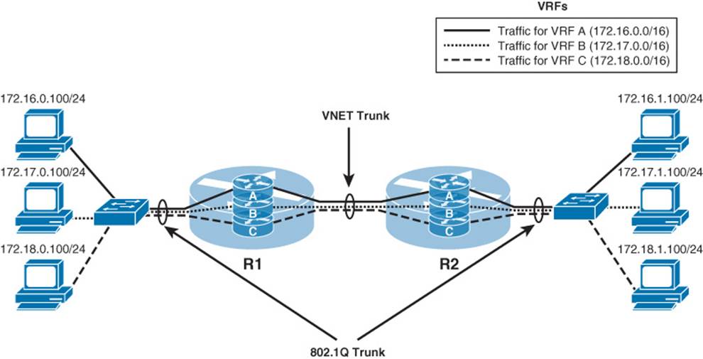
Figure 1-29 Sample EVN Topology
Even though an EVN allows a network architect to isolate one virtual network from another (as if they were physically separate networks), there is an occasional need for one of the virtual networks to be accessible by other virtual networks. For example, one virtual network might contain corporate DNS, DHCP, and email servers, which need to be accessed by all the other virtual networks. Cisco EVN makes this possible through a service called route replication. The route replication service allows IP routes known to one virtual network to be known to other virtual networks. As an example, consider Figure 1-30.
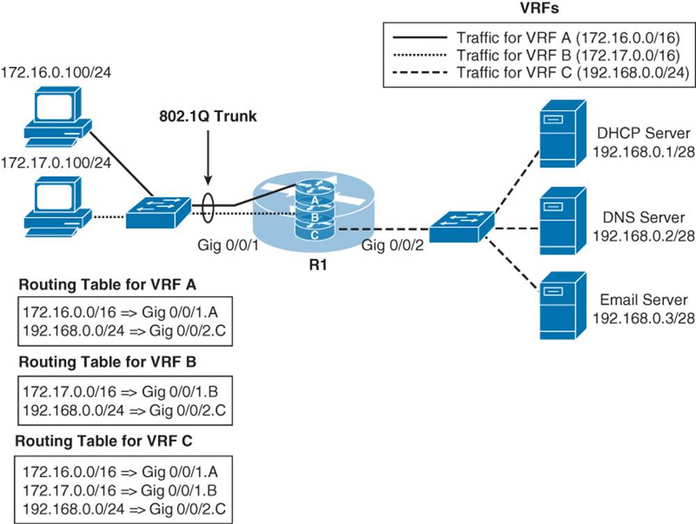
Figure 1-30 Route Replication
In Figure 1-30, the 172.16.0.0 /16 virtual network (VRF A) and the 172.17.0.0 /16 virtual network (VRF B) are isolated from one another. However, the 192.168.0.0 /24 network (VRF C) contains servers (for example, DHCP, DNS, and email servers) that need to be accessed by both VRF A and VRF B. Route replication allows networks in VRF C to be added to the routing tables of VRF A and VRF B, while still keeping VRF A and VRF B separate from one another. Also, notice that the routing table for VRF C knows about routes in the other two VRFs.
Note
Even though different IP address spaces were used in this example for VRF A and VRF B, in the real world, you could have overlapping address spaces in different VRFs.
Exam Preparation Tasks
Planning Practice
The CCNP ROUTE exam expects test takers to review design documents, create implementation plans, and create verification plans. This section provides some exercises that can help you to take a step back from the minute details of the topics in this chapter so that you can think about the same technical topics from the planning perspective.
For each planning practice table, simply complete the table. Note that any numbers in parentheses represent the number of options listed for each item in the solutions in Appendix F, “Completed Planning Practice Tables.”
Design Review Table
Table 1-3 lists several design goals related to this chapter. If these design goals were listed in a design document, and you had to take that document and develop an implementation plan, what implementation options come to mind? You should write a general description; specific configuration commands are not required.
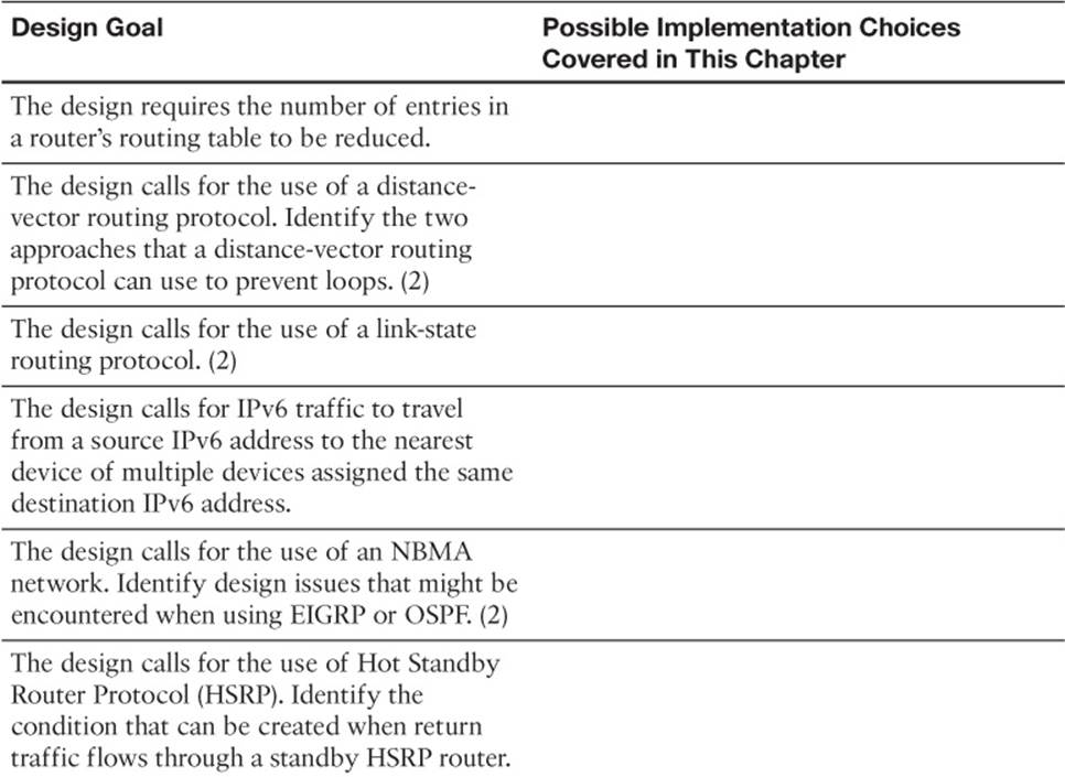
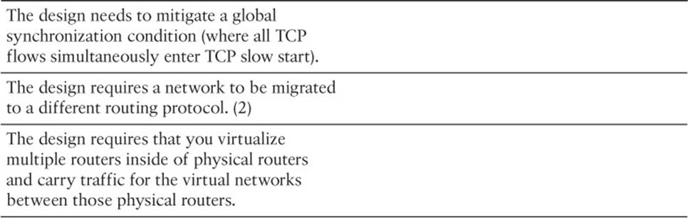
Table 1-3 Design Review
Implementation Plan Peer Review Table
Table 1-4 shows a list of questions that others might ask, or that you might think about, during a peer review of another network engineer’s implementation plan. Complete the table by answering the questions.
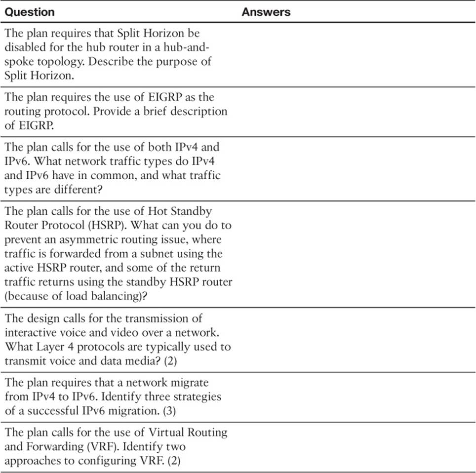
Table 1-4 Notable Questions from This Chapter to Consider During an Implementation Plan Peer Review
Review All the Key Topics
Review the most important topics from inside the chapter, noted with the Key Topic icon in the outer margin of the page. Table 1-5 lists a reference of these key topics and the page numbers on which each is found.
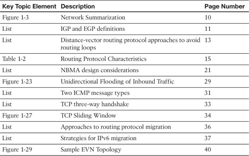
Table 1-5 Key Topics for Chapter 1
Complete the Tables and Lists from Memory
Print a copy of Appendix D, “Memory Tables,” (found on the CD) or at least the section for this chapter, and complete the tables and lists from memory. Appendix E, “Memory Tables Answer Key,” also on the CD, includes completed tables and lists to check your work.
Definitions of Key Terms
Define the following key terms from this chapter, and check your answers in the glossary.
convergence
route summarization
interior gateway protocol (IGP)
exterior gateway protocol (EGP)
distance-vector
link-state
path-vector
anycast
nonbroadcast multiaccess (NBMA)
Split Horizon
Poison Reverse
asymmetric routing
Administrative Distance
Easy Virtual Networking (EVN)