IPv6 Address Planning (2015)

Part III. Maintenance

Chapter 10. Keeping Your IPv6 Addresses Reachable

A name indicates what we seek. An address indicates where it is. A route indicates how we get there.

— Jon Postel

Introduction

There wouldn’t be much point to the whole exercise of creating and managing a great IPv6 address plan if we didn’t also implement policies and practices that keep those addresses reachable.

Routing on our internal networks and across the Internet requires some considerations unique to IPv6. We’ll review the IPv6 versions of the routing protocols familiar to us from IPv4 with special attention to the differences that will help us keep our IPv6 addresses live.

Many enterprises (especially small to medium-sized organizations) have traditionally relied on PA IPv4 space from an ISP. They may be opting for an IPv6 PI allocation directly from a RIR for the first time. The practices to keep those IPv6 prefixes externally reachable and optimally routed may be less familiar to them.

We’ll also examine the impact of IPv6 routing table size on memory that may affect the overall reachability of our networks.

Routing with IPv6

Just as with IPv4, you’ll be relying on a routing protocol to get traffic between sites or within sites. Thankfully, for the sake of preserving our copious amounts of free time (CAFT), we don’t have to learn any new routing protocols exclusive to IPv6. That is, the IGPs and EGPs we know and (as long as we’ve configured them correctly and they’re behaving) love from IPv4 have all been enhanced to support IPv6.

These include:

§ IGPs

§ RIPng

§ EIGRP for IPv6, IPv6 Implementation Guide, Cisco IOS Release 15.2M&T — Implementing EIGRP for IPv6.

§ OSPFv3^[127^]

§ IS-IS for IPv6^[128^]

§ EGPs

§ MP-BGP^[129^]

Figure 10-1 provides a comparison between the IPv4 protocols and the newer IPv6 versions.

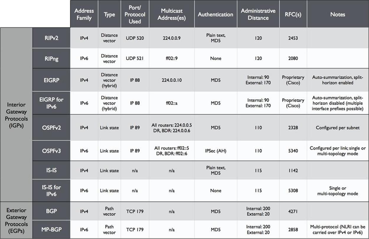
Figure 10-1. Routing Protocols Comparison, IPv4 to IPv6

We’ll leave any exhaustive exploration of these protocols to other, more worthy texts. But to explore some of their important operational considerations, we’ll need to at least briefly review them.

Selecting Your IPv6 Routing Protocol(s)

If you haven’t already been through this exercise and selected your IPv6 routing protocols (or even if you have and want to validate your choice), how do you go about choosing? Since we have at our disposal all the same routing protocols as in IPv4, one path forward is simply to select the one(s) we’re currently using.

As we’ll see, this approach is perfectly valid, but shouldn’t be made without examining some of the other considerations that should inform our choices based on how they may impact our operations.

But first, let’s look at the primary benefit of using the routing protocol (or protocols) we’re already using.

Operational Continuity

Using the same routing protocol(s) in IPv6 that we’re currently using in IPv4 has the powerful benefit of providing operational continuity. Since you and your colleagues are probably intimately familiar with how to keep whatever protocol you’re using today up and routing packets, you’ll be taking advantage of some institutional knowledge that should lead to (in theory at least) better and faster fault isolation and route optimization.

Even if we choose to run the same routing protocol for IPv6, there may be additional considerations (and gotchas).

Distance Vector and Link State Routing Protocols

Before getting into the difference between topology modes, let’s briefly review how dynamic routing protocols accomplish tracking network paths and routing packets. The most widely deployed routing protocols generally fall into one of two classes (or, in one case, a combination of both):

§ Distance vector

§ Link state

Of course, the goal of either of these types of routing protocols is to converge (and reconverge) quickly enough to create a stable, loop-free topology that gets packets from where they are to where they need to be in the network.

A distance vector protocol relies on each routing node sharing its entire routing table with all of its directly connected neighbors. The distance in distance vector is a measurement of the cost (often, the number of hops) to reach a destination, and the vector is via which next-hop router. Routers running a distance vector protocol pass along a routing table from one neighbor to another, i.e., “routing by rumor.”

RIP and EIGRP are examples of distance vector routing protocols.

By contrast, a node in a link state protocol knows about its directly connected links and shares these link states with its immediate neighbor nodes. Each node uses that information to build and maintain a link state database and calculate the shortest path to any given destination for a packet or flow. The reliability of this route information is generally much greater than its equivalent in a distance vector protocol because no router is sharing more than what it knows about directly and every node has calculated a complete picture of the network.

OSPF and IS-IS are examples of link state protocols.

TIP

One significant variation of the distance vector protocol is known as the path vector protocol. A path vector protocol associates each destination prefix with a particular path through the network. This path is formed by the chain of autonomous system numbers that would be traversed by a packet to reach the destination prefix. The path vector algorithm analyzes each path and removes any destination prefix with a path that contains the same ASN two or more times (implying a loop in the topology). BGP is an example of a path vector protocol.

EIGRP is primarily a distance vector protocol, but shares some features with link state protocols, such as neighbor state tracking and triggered updates (versus periodically sending the entire routing table). This provides for much faster convergence and a more reliable picture of the network.

ALL OF ‘EM

Years ago I worked for a large ISP that had several smaller ISPs as customers. One ISP customer in particular always seemed to be suffering outages and, as a result, initiated many calls to our NOC for emergency help. During one such troubleshooting session with this customer, I asked him what routing protocol or protocols he was running. “All of ‘em,” he replied (which, at the time and in his case meant RIP, OSPF, EIGRP, IS-IS, and BGP). My laugh was cut short by the realization that he was serious (and that this fact of his, um, network configuration was likely the source of his many, many outages). If only he’d been an early adopter of IPv6: he could have tried running no fewer than 10 routing processes!

Dual-Stack…but Not Necessarily Dual Topology

When it comes to choosing the IGP we’re going to use in a dual-stack environment, there’s an additional consideration that may not be immediately obvious. It’s based on the fact that two of our IGPs (as well as our EGP) provide a way to either share or isolate elements of the topology and (any associated router processes) according to what address family they belong to, i.e., IPv4 or IPv6.

Most current implementations of router and switch code available from Vitamin C, J, and B (i.e., Cisco, Juniper, and Brocade) vendors offer these options. Such options vary in scope and implementation, depending on the routing protocol in question, so let’s review each.

IS-IS for IPv6: Single-topology or Multi-topology Mode

IS-IS for IPv6 offers a choice of single-topology or dual-topology mode.

In single-topology mode, routers participating in IS-IS share a single link state database. Thus, the IS-IS process in this case bases its best path selection for both IPv4 and IPv6 routes on a single shortest path first (SPF) calculation for that database.

CAUTION

Keep in mind that this means anywhere you’ve configured an interface for IPv4, you’ll need to configure the same interface for IPv6 (and vice versa).

Because of this, the two protocols are sometimes said to share the same fate. Link-state changes that might normally only affect one protocol can cause an SPF recalculation and network reconvergence that affects both the IPv4 and IPv6 network.

By comparison, a router configured for IS-IS multitopology mode performs a separate SPF calculation for each protocol, isolating reconvergence and eliminating fate-sharing — at least as a consequence of routing protocol configuration and activity. After all, routers can still lose power! Because of this isolation, having disjointed sets of interfaces configured for IPv4 and IPv6 is perfectly fine.

So if you’re using IS-IS, which mode should you choose? Beyond the criterion of operational consistency that we already mentioned, the above described behavior has at least two consequences to consider:

§ Router resource preservation

§ Isolation and fault tolerance

Since single-topology mode maintains and performs SPF calculations on a single link state database, both router memory and CPU are conserved. Therefore, if the availability of these router resources in your dual-stack network is scarce, it might conceivably be necessary to run IS-IS in this mode.

By contrast, because mutlitopology uses two separate link state databases, each with its own SPF calculations, isolation and fault tolerance for each address protocol is better accomplished.

TIP

My recommendation is to run multitopology mode wherever possible. Any interruption to the production IPv4 network during the initial deployment of IPv6 can result in delays and setbacks to its adoption. By running multi-topology mode, the inevitable misconfiguration of IPv6 as it’s deployed in routing infrastructure will ideally only affect IPv6 traffic (and vice versa once IPv4 is officially the legacy protocol on your network).

OSPFv3 Address Families

The version of OSPF we’re likely most familiar with is version 2. This has traditionally been the IGP of choice among larger enterprises, especially where the greatest degree of interoperability between different vendors is desired.^[130^]

Version 3 of OSPF relies on the same basic link-state algorithms, but its link-state advertisements (LSAs) and packet formatting have been updated to accommodate the larger address size. It also leverages the IPv6 link-local address to form adjacencies. And since it’s per link instead of per subnet (and since IPv6 is designed to permit configuration of multiple IPv6 addresses and subnets per interface), a single link can support more than one instance of it.

For our discussion, the most important feature of OSPFv3 is that it allows for multiple address families. Let’s look at an example of this with an OSPFv3 configuration (Figure 10-2) — in the syntax of our favorite Vitamin C vendor.

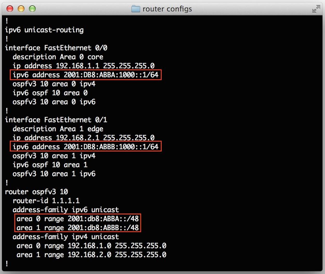
Figure 10-2. OSPFv3 router config example

Similar to IS-IS for IPv6 single-topology mode, all routers running a particular OSPFv3 process share a link-state database and SPF calculation. Thus, where maximum isolation and fault tolerance is desired, it’s perhaps preferable to run OSPFv2 for IPv4 and OSPFv3 for IPv6.^[131^]

MP-BGP

MP-BGP, or Multi-Protocol BGP, is an extension to BGP that allows BGP to carry Network Layer Reachability Information (NLRI, i.e., IP prefixes being advertised by a BGP peer) for multiple routed prototols — most importantly for our discussion, IPv6 and IPv4.^[132^]

MP-BGP shares configuration syntax with OSPFv3 in the form of address families. Because MP-BGP extenstions allow for multiple network protocol types, it is possible to send and receive IPv4 and IPv6 NLRI to and from a given peer over a single peering session of either protocol.

But the configuration preferred in nearly all cases is a peering session each for IPv4 and IPv6 to a given peer. As with our IGPs, it’s usually better to have isolation and fault tolerance than to, in the case of MP-BGP, save a few lines of configuration (as well as preserve a negligible amount of memory and CPU).

Figure 10-3 shows an example of an MP-BGP router config with the preferred configuration (separate peering sessions to the same external router and AS for IPv4 and IPv6).

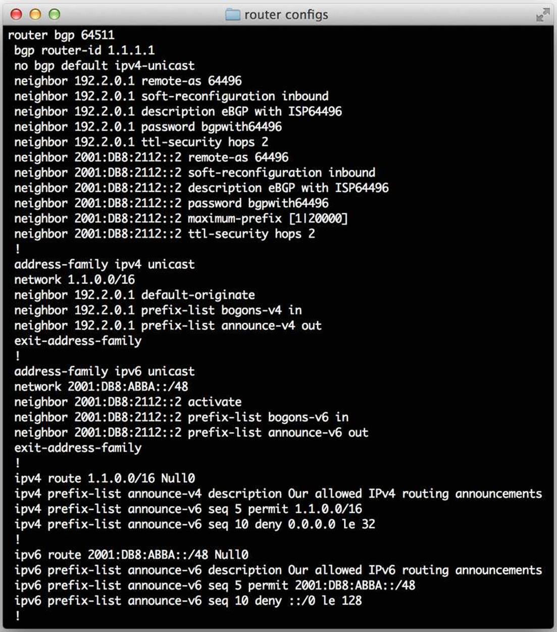
Figure 10-3. MP-BGP router config example

Routing Table Size and TCAM Space

Routing protocols provide a picture of the current network to all the connected and participating routers (as well as the hosts attached to them). The more complete and up-to-date this picture, the more flexibility an engineer may have to shape routing policy to improve network performance, lower costs, and reduce or eliminate outages (and successfully sleep through the night without getting called by the NOC!).

How this picture of the network is created and applied to routing and packet switching has changed (and improved) greatly over the years. As we’ll see, there is at least one aspect of IPv6 adoption that is problematic as a result of the current practice. But first, let’s briefly review how we got here.

RIB versus FIB

A RIB, or routing information base, is essentially the routing table on a router. A router could have a number of ways of determining what networks are reachable to it, including the ones that are added as static routes, the ones that are directly connected, or the ones that are learned via a dynamic interior gateway protocol (IGP) like OSPF or EIGRP. Since every valid destination network is paired with at least one next hop or outgoing interface, routers must have some mechanism for determining the availability and desirability of one or more of these exit points. Most routing protocols provide this, but BGP, as well as some static routes, can have a next hop that is not directly reachable. This requires that the router perform a recursive lookup for these “remote” next hops. Because of this, it’s not always possible to directly switch a packet without at least one recursive lookup.

Very early routers would look up the destination for each packet in the routing table and send it on its way.

Obviously, this process was very CPU- and memory-intensive and generally inefficient — especially for more modestly sized networks with a small number of unique destinations. Fast switching was created to increase the performance and efficiency of routing by caching the results of a recursive lookup so that ensuing packets to those same destinations wouldn’t need to be processed by the router CPU but could be fast-switched instead. This was accomplished by copying the RIB to a forwarding information base (FIB) that didn’t rely on process switching but could be pushed down to the port, along with the any cached next-hops, for fast packet switching.

FIBs are stored at the port level in something called ternary content addressable memory, or TCAM (alternately spelled $$$). Because TCAM is expensive, it is usually limited in size, meaning the number of supported FIB entries is subsequently limited as well. This means that the picture of the network on a given port might risk being incomplete if all the routes needed to complete that picture won’t fit because of limited memory.

Complicating this is the continued growth of the IPv4 routing table, which now contains over 512,000 IPv4 prefixes (Figure 10-4).^[133^] As the impact of IPv4 exhaustion begins to be felt, more organizations will be looking for ways to sell some of their existing allocations. This will result in more /24s being carved out for deployment along with the precipitous increase in routing table size this results in.

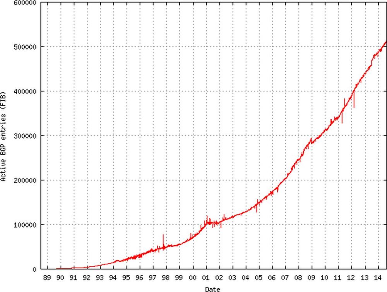
Figure 10-4. Global routing table, number of prefixes (Source: The CIDR Report)

Enter IPv6. One consequence of the adoption of IPv6 is a four-times increase over IPv4 in the amount of TCAM required for an IPv6 address entry, e.g., 32 bits for an IPv4 address, 128 bits for an IPv6 address. But wait, couldn’t some memory be conserved by reserving only 64 bits of addressing for IPv6, given that we generally don’t keep track of networks for routing for those prefixes smaller than a /64 in prefix size? Don’t forget that we still have to accommodate networks for point-to-point links and loopback interfaces. Also, it’s possible that some future IPv6 network architecture or configuration might rely on a network smaller than a /64, yet not one of the well-known exceptions to the no subnets smaller than a /64 rule.

Since most ports are doing double duty supporting dual-stack, this has resulted in the necessity of creating profiles for the TCAM available on a given port. Such profiles require the engineer to pre-partition the available TCAM, allocating some TCAM for IPv4 routes and some for IPv6. If the architecture requires a higher degree of routing visibility and policy granularity for a particular interface (e.g., one of two or more egress ports to the Internet), a larger amount of TCAM may be needed.

As mentioned, the DFZ for IPv4 contains more than 512,000 routes. The IPv6 Internet routing table contains more than 18,000, which, when mutliplied by the at-least-two-times factor based on the bits required by the network portion of the larger address, is the equivalent of no fewer than 36,000 IPv4 prefixes. 512K is a common TCAM size and obviously insufficient to hold all DFZ IPv4 prefixes, much less the combined prefixes for both the IPv4 and IPv6 global routing table. For example, 512,000 IPv4 routes + 18,000(x2) IPv6 routes = 548K routes. As TCAM must be partitioned according to the rules of binary arithmetic, a profile for 512K of TCAM might provide 384K for IPv4 and 128K for IPv6.

While the current IPv6 global routing table would consume only half of the available partition, the IPv4 partition would be at 132% utilization, resulting in the unreachability of some significant portion of the IPv4 global routing table.

Increasing the TCAM size to, say, 1M provides both adequate memory for current IPv4 and IPv6 global routing tables, as well as additional memory overhead to accommodate the inevitable growth of the IPv4 and IPv6 routing tables. But with the greater expense of additional TCAM, you’ll need to verify that the enhanced egress traffic control (with the more complex routing policy associated with it) is justified by the existing network architecture. For example, an enterprise would need to be multihomed to at least two providers to take advantage of such policies (and the extra visibility receiving the full routing table for both address families affords).

Mars Needs IP Address Blocks

A big part of keeping your IPv6 addresses reachable on the Internet is keeping your routing table free of Martians, bogons, and fullbogons. And by the way, keep in mind that all bogons are now Martians but not fullbogons.

Wait, what?!

Don’t panic! In case you didn’t know, all of these are merely somewhat whimsical idioms for bad (i.e., bogus) IP addresses and prefixes. So what’s the difference between them (and what’s the etymology of these somewhat silly terms)?

Martian

A Martian is any reserved or private address block.^[134^] We’re likely most familiar with these from IPv4 as private addresses defined in RFC 1918.^[135^]

IPv6 Martians can be found in RFC 5156, Special-Use IPv6 Addresses, some prefixes of which we reviewed in Chapter 2. Table 10-1 shows the full list.^[136^]

Table 10-1. IPv6 Martians

Bogons

A bogon includes not only all Martians but also space that hasn’t been allocated by IANA yet to a RIR. A bogon list can be generated by reviewing both IANA’s updated list of reserved and allocated prefixes, as well as the combination of lists of prefixes not yet assigned by IANA to the RIRs. However, Team Cymru maintains a list of bogons and fullbogons (explained below) that can be retrieved manually or automatically using an Internet routing registry (IRR).^[137^]

Fullbogons

A fullbogon is a concept (and accompanying list) invented by Team Cymru after they realized that the existing bogon lists were not granular enough, given that they didn’t also contain allocations from IANA to the RIRs that had not yet been assigned to ISPs or end-users.

Attack of the Bogons!

At this point, you may be asking yourself (if you don’t already know from bitter experience), what’s so bad about bogons anyway?

Black-hat hackers and assorted reprobates use bogons to provide spoofed source addresses to enable denial-of-service (DoS) and distributed denial-of-service (DDoS) attacks. Any Internet routability of bogon prefixes makes such malicious efforts easier.

The miscreants responsible for these attacks would like nothing better than to have a new network protocol at their disposal — especially one for which operational and security standards are still maturing, leaving potential paths of exploit open and available.

It’s incumbent on all of us deploying IPv6 for the first time to make sure that we maintain (or even improve) our security policy and enforcement in IPv6.

What this means in the context of our current topic is making sure that you properly filter bogons (preferably inbound and outbound) at your Internet edge.

BOGON ETYMOLOGY

So how does a peculiar little word like bogon come into existence anyway?

Well, according to programmer, hacker, and sys/netadmin lore, bogons are the quanta of the property of being bogus (i.e., bogusness, or bogosity if you prefer). Further clarification for the ESL set: bogus has traditionally meant fake or counterfeit, but according to some American slang has come to mean undesirable or useless (i.e., “suckiness”) in slang. Network folks have apparently found a nice overlap of the traditional definition and the slang one in the fact that a bogon prefix is used to counterfeit packets and create general, shall we say, suckage.

Filtering Bogons

So how do we go about filtering bogons in IPv6? Before we look at the specifics, let’s briefly review the general architecture and configuration to which such filtering is applied.

Unless you’re running a service provider network with lots of peers and IP transit connections to the Internet, chances are you are connected to one or two (a few at the most) ISPs.

Those among us running singly-homed networks probably needn’t worry about edge filtering because, in all but the most unusual cases, they wouldn’t be running BGP. Instead, they would typically have static routes for both Internet ingress and egress. Incoming traffic would be routed to their network by a route on the ISP side. Outgoing traffic would be routed by a default route to the Internet.

However, where a network is dual- or multihomed and using BGP to share routes with two or more upstream ISPs, proper prefix filtering is a must.

Figure 10-5 shows an enterprise network customer multihomed to two providers.

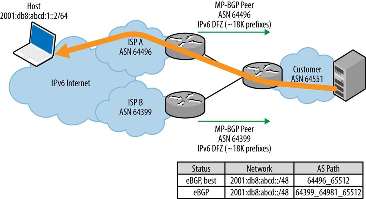
Figure 10-5. Egress route optimization, multihomed network

Say the enterprise customer would like to be able to control outbound traffic flows and send them via ISP A or ISP B, depending on performance, based on the shortest path, to a particular flow’s destination, e.g., in the figure’s example, responding to a request for content from a host located at the address 2001:db8:abcd:1::2/64.

For traffic optimization, the customer would need to be configured, and have sufficient router memory, to receive the entire global routing table. As discussed earlier in the chapter, there are currently slightly more than 500K routes for IPv4 and more than 18K routes for IPv6. The full table allows the enterprise content server to select the best egress path, e.g., shown in the figure as the path to the host through ISP A).

In instances where basic redundancy is desired (or router memory is insufficient), the customer could instead receive a default route from each ISP and preference an outbound link, according to criteria like best performance or price (Figure 10-6).^[138^]

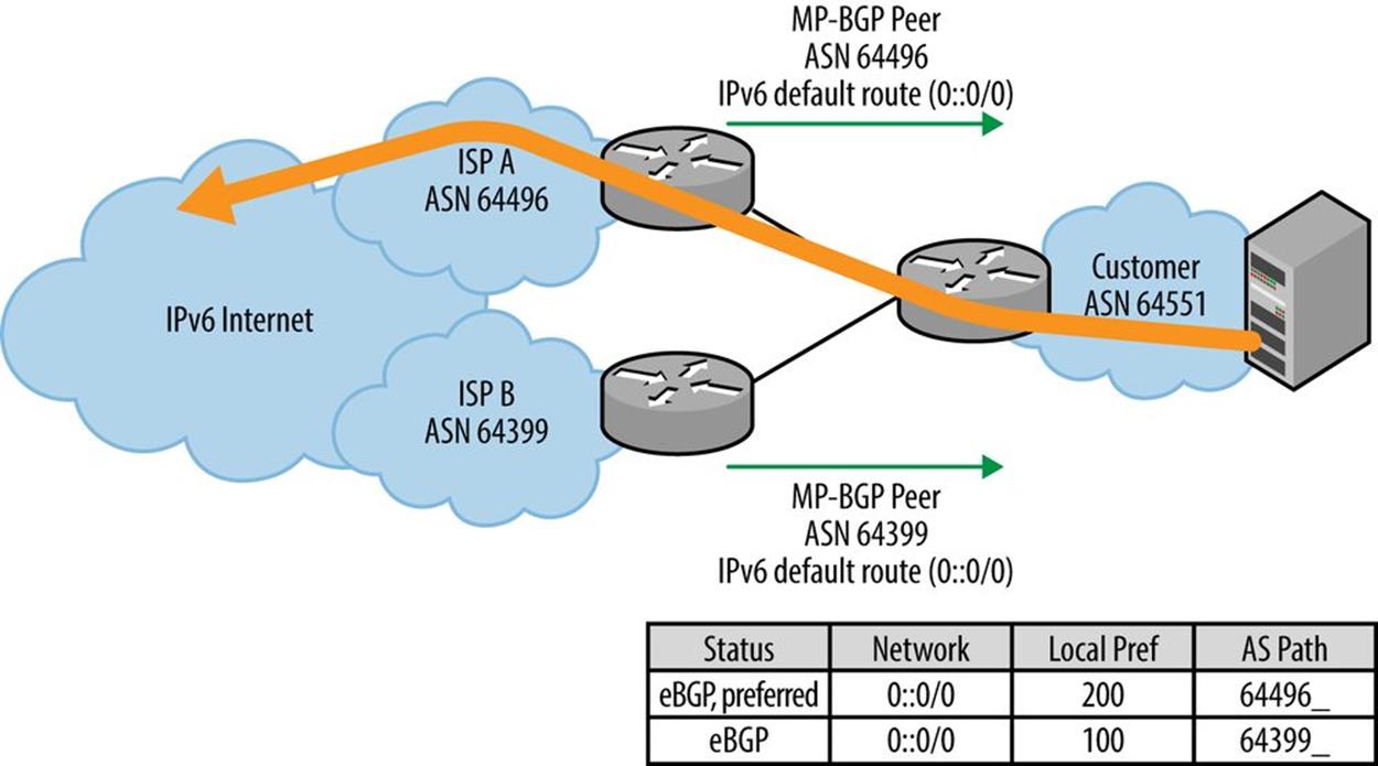
Figure 10-6. Basic redundancy, multihomed IPv6 network

In either case, the customer would need to be configured to advertise its IP netblock(s) to both ISPs, providing redundancy and more optimal performance for inbound traffic.

Bogon filtering is configured for both sent and received routes on the customer’s BGP sessions with each of the ISPs. If they are adhering to best practices, the ISPs will likewise be filtering the routes they send to, and receive from, the customer.^[139^]

Note that the provider’s outbound announcement immediately becomes the customer’s received routes, just as the customer’s become the provider’s. Thus, in an ideal world, a perfectly maintained bogon filter applied outbound on the provider’s BGP configuration and session would preclude the need for a bogon filter on the customer’s inbound BGP configuration (and vice versa).

So if you trust your provider as you would your brain surgeon, feel free to leave that ingress filter off. After all, it’s one less configuration you’d have to deal with. While you’re at it, see if you can convince your provider that you’ll keep your filters up-to-date with the latest bogons and meticulously applied so the provider can do the same. What could possibly go wrong?

Mild sarcasm aside, bad routes filtered at your provider’s egress would never clutter up your link to the ISP before being dropped anyway when received by your router and filtered by what should be, in an ideal world, the exact same filter.

But as we know, in the less-than-ideal world of network operation, we can’t guarantee that our ISP will never accidentally advertise bogons to us, any more than we can guarantee our ISP that some fat fingers or a security breach on our end won’t result in us announcing garbage to them.

Thus, for the best security, bogon filters should be applied to our sent and received BGP routing advertisements. And the more complete and up-to-date the bogon list, the better the protection.

Table 10-2 summarizes filter sources in order of completeness.

Table 10-2. Filter sources, from least to most complete

As you’ve probably inferred, the list of netblocks allocated by IANA to the RIRs, as well as the netblocks allocated to the RIRs but not yet assigned to ISPs or end-users, changes over time.

For example, since IANA handed out the last of the unallocated IPv4 netblocks back in 2011, bogons now include only martians. But the fullbogons list will continue to change. As a result, our filters need to be updated often enough to track and accommodate these changes.

Perhaps the best way to keep up with changes is to automate the whole process by peering with a bogon list maintainer (e.g., Team Cymru) or an IRR (e.g., RADb). Such a configuration is beyond the scope of this book but can be found on the Team Cymru website.

Finally, the appropriate filtering logic for catching IPv6 bogons is a bit different than it is in IPv4. The reason is that the list of fullbogons for IPv6 is in the neighborhood of 50K prefixes,^[140^] and is around 20 times larger than the list for IPv4.

More than 50K entries is a whole lot of config real estate and, unless maintained automatically, an opportunity for incorrect new entries or changes with typos. As a result, it makes more sense to explicitly allow only the known valid IPv6 prefixes while implicitly denying everything else (Figure 10-7).

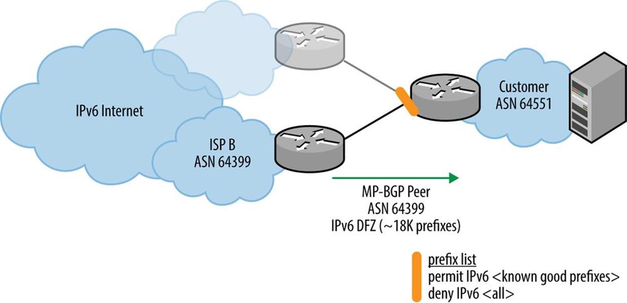
Figure 10-7. Fullbogon filtering in IPv6

This is the reverse of the filtering logic we apply in IPv4 with its more manageable fullbogon list: explicitly deny the bogons while implicitly allowing everything else (Figure 10-8).

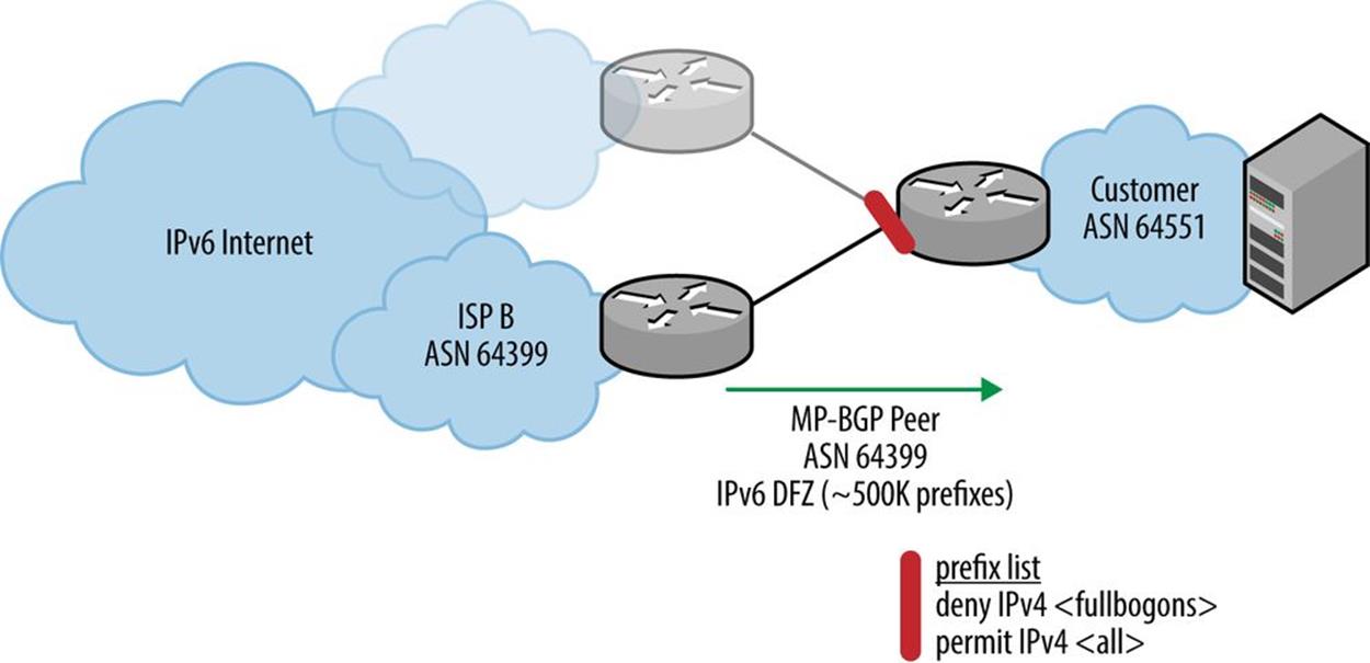
Figure 10-8. Fullbogon filtering in IPv4

Summary

In this chapter, we covered some of the critical operational aspects of keeping the prefixes of your IPv6 address plan reachable.

As we’ve learned, the routing protocols we’re most familiar with from our IPv4 operational environments all have IPv6 versions. But we’ll need to take care to select the right one based on balancing the need for operational continuity with the need for IPv4 production network stability. The former is arguably provided best by using the same routing protocol for IPv6 as we use for IPv4 (along with perhaps single-topology mode where available and required by any limits on router resources). Meanwhile, using a different routing protocol (or dual-topology mode) may provide better isolation and fault tolerance of both IPv4 and IPv6 networks (but especially the existing IPv4 production network).

Proper filtering of routes received from, and announced to, your ISP will also help keep your IPv6 network prefixes reachable. We covered the differences between bogon lists in the respective address families and the contrasting filtering logic required to catch them. We also need to ensure that we’re not announcing garbage to our peers, even if it’s just our upstream ISP.

^[127^] RFC 5340, OSPF for IPv6.

^[128^] RFC 5308, Routing IPv6 with IS-IS.

^[129^] RFC 4760, Multiprotocol Extensions for BGP-4.

^[130^] As a result of such wide deployment, there is a tremendous amount of collected operational wisdom on how OSPF behaves in production that can be leveraged by engineers and operational staff.

^[131^] RFC 5838, Support of Address Families in OSPFv3.

^[132^] The extensions in MP-BGP also allow for carrying NLRI for MPLS VPN and multicast.

^[133^] As of Tuesday, August 12th, 2014: “The Internet Just Broke Under Its Own Weight…”.

^[134^] Nothing should ever originate from the Red Planet!

^[135^] We may be less familiar with the other two RFCs that define Martians in IPv4 — RFC 5735 (i.e., Special Use IPv4 Addresses) includes all the other reserved addresses along with those already defined as private in RFC 1918. Meanwhile, RFC 6598 (i.e., IANA-Reserved IPv4 Prefix for Shared Address Space) more recently defined a /10 of IPv4 addresses to share among those providers deploying CGN. Feel free to look up these additional ranges, as we won’t clutter up our beautiful IPv6 address planning book with more IPv4 addresses than necessary!

^[136^] Not all address ranges in RFC 5156 are Martians. For example, the Teredo prefix (2001::/32) and 6to4 prefix (2002::/16) may be advertised on the Internet where these services are offered.

^[137^] The Bogon Reference — Team Cymru. Team Cymru Research NFP describes itself as “a specialized Internet security research firm and 501(c)3 non-profit dedicated to making the Internet more secure…Team Cymru helps organizations identify and eradicate problems in their networks, providing insight that improves lives.”

^[138^] The customer might also opt to receive the network prefixes of the provider’s other customers along with the default route. While not requiring as much memory as the full table, this BGP policy at least ensures that egress traffic will select the provider with the shortest path to learned, more specific destination networks.

^[139^] Belt and suspenders, baby!

^[140^] This is more than twice as many entries as the actual IPv6 global routing table!