IPv6 Address Planning (2015)

Part I

Chapter 2. What You Need to Know About IPv6 Addressing

We’ll need to be familiar with the basics of IPv6 addressing as we learn and apply IPv6 address planning concepts and methods. If you already know this topic well, feel free to skip ahead to the next chapter.

Representation

Let’s review the basic representation of the IPv6 address. The IPv6 address is 128 bits long:

00100000 00000001 00001101 10111000 00000000 00010000 10101010 00100000

00000000 00000000 00000000 00000000 00000000 00000000 00000000 00000001

Easy to write, easy to remember — that is, if you’re a computer^[28^] or a savant.

For everyone else, it’s easier to manage in its usual form, presented as 8 hextets^[29^] (each with up to 4 hexadecimal values) of 16 bits, separated by colons:

2001:0db8:0010:aa20:0000:0000:0000:0001

NOTE

You’ll notice that we’re consistently using lowercase letters in our examples. IPv6 standards recommend lowercase letters when presenting addresses. But that’s just for human consumption: when formatting IPv6 addresses for internal storage in a database or application, uppercase, lowercase, or any combination of the two can be used. Also, various OSes and types of networking equipment may present (or allow for configuration of) an IPv6 address in either uppercase or lowercase with no impact on functionality. However, keep in mind that consistent address representation becomes important to find addresses in databases and spreadsheets more easily (especially if you don’t have, or can’t soon deploy, an IPAM solution). A good choice for such representation might be the full (i.e., 32-character) address with lowercase letters like the example shown previously.

Even better, we can simplify the presentation of the address by following two easy rules to shorten it:

1. Leading zeros in any hextet can be dropped:

2001:db8:10:aa20:0:0:0:1

2. One set of contiguous hextets of zeros can be replaced with a double-colon:

2001:db8:10:aa20::1

WARNING

Note that the second rule can only be used once per address. If you did it twice in an address, you’d have no way of unambiguously determining how many hextets had been replaced with each double-colon. And since you may have more than one group of contiguous zero hextets, it’s generally advised that you shorten the longest one.^[30^]

You may have noticed that after we apply the two rules to shorten our example, it has only two more significant characters than the longest possible IPv4 address. With a little planning, IPv6 addresses can often be just as easy to read and remember as IPv4. (But as we’ll see, most host addresses end up being much longer and require DNS to track and manage them more easily).

MIDNIGHT AT THE DEAD BEEF CAFE

If you’ve ever played Boggle™ (or any of its variants), you may have found it amusing to see how many words you can come up with, given a limited number of letters.^[31^] Because IPv6 addresses use hexadecimal representation, the letters a through f (along with numbers substituting for letters) are available to rearrange into recognizable words. Since IPv6 has been around for more than a decade, examples of this kind of word play are now common:

2001:db8:dead:beef::1

2001:db8:cafe:babe::A90

And so on.

The most famous practical example of this comes courtesy of a well-known social networking site:

2a03:2880:2050:3f07:face:b00c::1

Cute, but should any such addresses generally be used in production? As with any design decision, there are trade-offs to keep in mind.

It’s possible that it will be that much easier for operations personnel to keep track of network locations or functions by encoding recognizable and memorable words into IPv6 addresses or prefixes. (We’ll see a more general example of this technique later.)

But it’s also possible that malicious scans of IPv6 address space could be made easier with dictionaries of well-known words constructed using hexadecimal characters and common substitutions.

Security concerns aside, while possibly entertaining and memorable, such addresses aren’t generally flexible or scalable enough for a production network, but may be perfectly suitable when configuring IPv6 prefixes and addresses for lab environments and testing purposes (as well as making packet captures more readable for training or demonstration).^[32^]

Structure

So now that we’ve looked at how the 128 bits of the IPv6 address can be more manageably represented, let’s look at how those bits are structured.

Returning to the early days of Ye Olde IPv4e, recall that classful addresses, more specifically class A and class B networks, were the standard allocation sizes for most organizations. Early networks, though, were unlikely to need anywhere close to the 16.7 million class A (or even 65.5K class B) IP addresses for host addressing. From the standpoint of host addressing requirements, such extravagance is somewhat like asking for a new pair of pajamas for your birthday and instead getting a circus tent to wear to bed. It seems a bit short-sighted in hindsight given all the tweaking of subnets using VLSM and CIDR we’ve had to do in the intervening years. But as we’ve also already mentioned, the tremendous success and explosive growth of the Internet was still many years in the future.

In the meantime, sufficient host addressing was only one of the requirements of IP addressing anyway. The other requirement was met quite handily by all those class A and B allocations: namely, a hierarchy of consistently sized networks that made for simple prefix aggregation and efficient routing. This, in turn, kept the size of the global routing table manageable, improving routing stability, as well as conserving router memory and CPU cycles.

The idea was the right one; it’s just that the address space was not sufficiently large to support it once the Internet really took off. The 128 bits of IPv6 addressing, on the other hand, enables both network hierarchy and prefix aggregation, as well as sufficient host addressing, all without running out of bits.

The most basic structure of the IPv6 address is the division of the address into some number of network bits for the subnet prefix and some number of host bits for interface identification. While theoretically the interface ID could use as many bits as are left over after subtracting the network bits from the 128 bits available in the overall address, in practice, interface IDs are always 64 bits (with subnet prefixes necessarily having no more than 64 bits).^[33^]

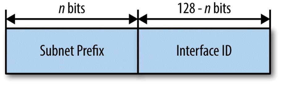
We’ll be focusing mainly on the network (or subnet prefix) portion of the address, as we’ll have a subset of those bits to work with in creating and maintaining our IPv6 address plan.

Keep in mind that IPv6 was designed to fully utilize 64 bits of host addressing. Thus, further subnetting the 64 host bits (i.e., the right half) of the IPv6 address is generally not recommended.

For one thing, address autoconfiguration mechanisms rely on a 64-bit host portion and can break if one tries to configure any subnets longer than 64 bits.

For another, when network architects new to IPv6 begin to think about what to do with all of the IPv6 space they’ve been allocated, a common reaction is the understandable desire to further divide the 64 host bits in order to reflexively conserve host addresses; just like the subnets they’re used to in IPv4 (i.e., “right-sized” using CIDR and VLSM for network segment host counts).

There are, however, a few special use cases with associated subnets where such further subnetting of the 64 host bits is appropriate. We’ll look at those later in the chapter.

Types

The original specification for IPv6 addressing defined three general types of addresses: unicast, multicast, and anycast.^[34^] The general description of each of these address types should be familiar from IPv4.

We’ll introduce slightly more formal definitions for each IPv6 address type, but perhaps the easiest way to think of them is by the communication between nodes they’re designed to enable, as shown in Table 2-1.

Table 2-1. Node communication by address type

Unicast Addresses

Strictly speaking, a unicast address goes on an interface and allows packets to be sent specifically to that interface. It’s convenient, and therefore habitual, to think of hosts as being configured with an address (or addresses). It’s equally common to think of unicast communication as taking place between two hosts rather than two interfaces. That’s perfectly appropriate for most situations. But if we want to get technical, in IPv6 a host is referred to as a node. Nodes can have any number of interfaces, but each is uniquely identified by at least one unicast address.

IPv6 unicast addresses contain several additional subtypes:

Loopback address

::1/128

First is the loopback address, already familiar to us from IPv4 (e.g., 127.0.0.1). It serves the same function in IPv6, allowing the node to send packets to itself.^[35^]

Link-Local unicast addresses

fe80::/10

Link-Local unicast addresses are defined by the first 10 bits of the address and are reserved for use on a single link. They play a critical role in Neighbor Discovery and auto-address configuration. They also provide for improved (i.e., largely automated) default gateway configuration and management (as compared with IPv4). A Link-Local address is automatically configured on an interface once the IPv6 stack is activated.^[36^]

Unique-Local unicast addresses

fc00::/7

Unique-Local unicast addresses (ULA) reserve the first 7 bits of the address and are sometimes described as being the equivalent of RFC 1918 (i.e., private) addresses in IPv4. In general, they are redundant where an organization has received a Global Unicast Allocation, or GUA (see the next entry).

Global unicast addresses

2000::/3

Next, the address range that we’ll be spending the most time with is global unicast addresses (GUA).^[37^]

TO ULA OR NOT TO ULA

Unique-Local addresses (ULA) merit a special discussion.^[38^] We need to understand their benefits and limitations and recognize when it’s appropriate to utilize them.

ULA are most often compared to RFC 1918 addresses in IPv4. This is a useful comparison as far as it goes, but IPv6 ULA offer some advantages over IPv4 private addresses.

The most obvious of these is more address space per site. The standard site allocation for ULA is the same as it is for GUA: a /48. Compared to the largest IPv4 private address allocation of 10.0.0.0/8, a /48 offers 7.2x10¹⁶ times the number of addresses!

The global ID defining a ULA site prefix is designed to be allocated in a pseudo-random fashion.^[39^] This means that unlike IPv4 private addresses, the probability of any two ULA prefixes overlapping is extremely low.

Since it’s very unlikely that ULA prefixes would be identical and contain overlapping space, consolidating networks after a merger or acquisition would be less problematic than in IPv4. Most organizations use the 10.0.0.0/8 space (often more than once in the same large network) and must rely on NAT or VRFs to overcome conflicting address space.

And just like all IPv6 site allocations, ULA prefixes can offer a well-defined /48 boundary that makes it easier to include in ACLs, either for routing policy prefix filtering and security policy firewall rules — as well as for IPv6-to-IPv6 Network Prefix Translation (NPTv6) use, something we’ll look at a little more closely in Chapter 9.

The similarities of Unique Local addresses with RFC 1918 space make them intuitively appealing for most enterprise network architects and engineers new to IPv6. Using RFC 1918 addresses along with NAT in IPv4 at the enterprise network edge is the de facto standard for most enterprises (and has been for well over a decade). As a result, it’s generally very well understood by network operations staff and well supported by vendors. Whatever its drawbacks (and there are keen ones), the practice of supporting IPv4 NAT and private addressing is quite mature.

Keep in mind, however, that IPv6 was designed to support multiple addresses (and address types) per interface. As a result, some organizations may wish to configure both ULA and GUA on the same host: The former for access to internal resources with the latter for Internet access.

This is the globally routable allocation that our organization will be assigned a block from by an RIR or an ISP. GUA allocations are of two types: provider independent (PI) and provider assigned (PA).^[40^] PI allocations are portable, meaning they can be announced and routed via any ISP. They are assigned by the RIR directly to an organization. PA allocations are assigned by the ISP and must be returned if switching to a new ISP, which requires network renumbering. PI and PA allocations are covered in more detail in Chapter 6.

Multicast Addresses

In contrast, a multicast address is assigned to and identifies a group of interfaces.^[41^]

Multicast addresses

ff00::/8

The multicast address range begins with all ones in the first eight high-order bits. (The next four bits set various flags used to help characterize the address.)

The four bits that follow create various multicast scopes, i.e., the scope of the network the addressed packet is destined for. Multicast scopes are shown in Table 2-2.^[42^]

Table 2-2. Multicast scopes

For operational purposes, the multicast addresses (and scopes) we’re likely to interact with most frequently are displayed in Table 2-3.

Table 2-3. Common multicast addresses

With the first 16 bits of the multicast address spoken for, 112 bits remain for multicast group IDs (that’s 5.2x10³³ available groups per multicast prefix!).

Anycast Addresses

An anycast address is also assigned to multiple, different interfaces, but packets are delivered to the interface closest to the sender, as determined by routing metrics. Thus, an anycast address can actually be any unicast address.

Both IPv6 and IPv4 anycast addresses are used by large network operators in their WAN (or even global) DNS designs. Name servers maintained by these operators are configured with anycast addresses, and end-user DNS queries are then routed to the closest name server. This generally succeeds in improving overall session performance.^[43^]

Finally, not technically included in any of the above three types is the unspecified address.

The Unspecified Address

Unspecified address

::/128

This is an all 0s address. It signifies that the node doesn’t yet have an address and, as such, is used as the source address in any IPv6 packets sent by a node before it has learned its own address.

Figure 2-1 compares the different IPv6 address types.

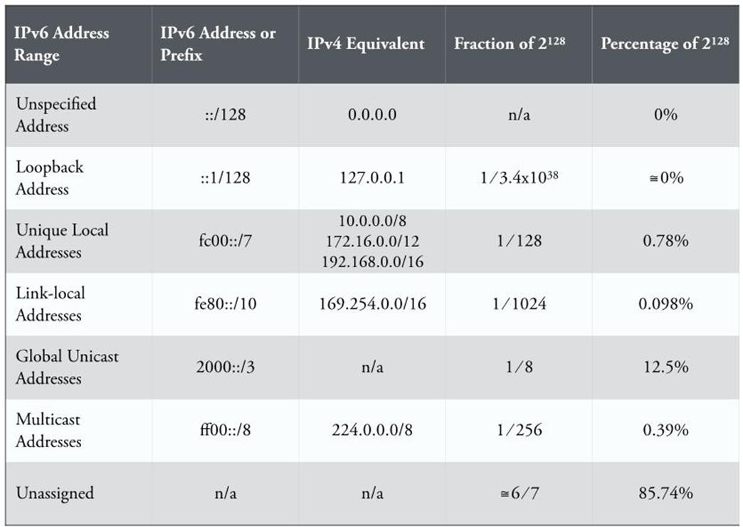
Figure 2-1. IPv6 address ranges

IPV4-MAPPED ADDRESSES IN IPV6

In the early days of IPv6, a fair amount of effort was expended in finding ways to translate IPv4 addresses into IPv6 ones. Some of these methods were merely representational, while others were coded into actual transition mechanisms. In general, such methods have either not been widely adopted or have fallen out of favor, as they most often end up being more operationally taxing and much less manageable than a green-field dual-stack deployment.

Still, it’s important to be aware of the methods that exist for representing or translating IPv4 into IPv6. We often end up responsible for networks we didn’t design or build. Such networks may include one or more of these approaches, and we may need to manage them and develop a plan for their eventual replacement.

There are two IPv6 address types that have embedded IPv4 addresses. Either may be in use in an existing IPv6 network and may show up in an existing address plan (or IPAM system):

§ IPv4-compatible addresses

§ IPv4-mapped addresses

IPv4-compatible addresses

An IPv4-compatible address looks like this:

0:0:0:0:0:0:192.0.2.234

Because of the six repeated, leading 0 hextets, sometimes these addresses will be represented in this potentially confusing format:

::192.0.2.234

All of these addresses are to be found in the range ::/96

In any case, as we can observe, the left-most 96 high-order bits are set to 0 with following 32 low-order bits set to the IPv4 address.^[44^]

The original idea with these addresses was to create a dynamic transition mechanism where IPv6 packets would be tunneled over IPv4 networks. But IPv4-compatible addresses have been deprecated, which is the IETF’s rather fanciful way of saying they’re no longer to be supported by vendors or deployed in the wild. If they’re in use in a network you administer, be aware that they won’t be supported in any new hardware or software. You’ll most likely want to decommission them as soon as reasonably possible.

IPv4-mapped addresses

An IPv4-mapped address looks like this:

0:0:0:0:0:ffff:192.0.2.234 (or, ::ffff:192.0.2.234)

These addresses are assigned from the range ::ffff:/96

The left-most 80 high-order bits in an IPv4-mapped address are set to 0, while the next 16 bits are set to 1 (ffff). The following 32 low-order bits are set to the IPv4 address.

While not formally deprecated, IPv4-mapped addresses are not commonly used.

Protocol Improvements

Recall that there were two primary reasons for developing IPv6. First, and most obvious, was the need to overcome address scarcity, given the limited 32-bit address space of IPv4. The second reason was to provide more consistent hierarchy and thus more efficient routing on the Internet. But the early decision to forgo backward compatibility with IPv4 meant that the designers of IPv6 also had leeway to make some additional improvements to the new protocol. These improvements include:

Simplified packet headers

IPv4’s variable-length header has been replaced in IPv6 with a fixed 40-byte header. As a result, IPv6 packets are processed more quickly by routers and switches.

Improved header option and extension support

IP options have been relocated to appended header extensions, greatly increasing the flexibility, manageable length, and forwarding efficiency of IPv6 packets.

Flow labels

The ability to label packets as part of traffic flows that get special QoS processing by routers and switches has been integrated into IPv6.

Support for encryption and authentication

Authentication and Encapsulating Security Payload headers have been included as part of the general protocol specification.

Neighbor Discovery

ARP in IPv4 has been replaced with Neighbor Discovery in IPv6, which leverages Internet Control Message Protocol version 6 (ICMPv6) to provide a more efficient mechanism (multicast instead of broadcast) for mapping layer 3 to layer 2 addresses.

Other changes include built-in support for automatic host address configuration via stateless address autoconfiguration (SLAAC).^[45^]

As uptake of IPv6 has increased in production enterprise environments, and on the Internet, some of these changes have proven durable, while others appear to have an uncertain future. For instance, the fixed 40-byte header length in IPv6 (as compared to the variable-length header in IPv4) has greatly improved forwarding efficiency.

Meanwhile, flow labeling, while promising, has yet to be widely deployed and is mostly unused. Similarly, rarely used features like Mobile IP (which permit devices to maintain permanent IP addresses even while moving among different networks) have much better support in IPv6. Finally, protocol attacks on extension headers have led to proposals that some of them be deprecated.

Though it’s definitely recommended that you explore these improved features thoroughly as part of your overall IPv6 training, we’ll go ahead and leave the gory details to other texts (except where they may directly impact IPv6 address planning).

Subnetting Host Bits

We mentioned earlier that there are situations where it’s appropriate to subnet the 64 bits of the host portion of the IPv6 address. Typically, there are two such cases:

1. Loopback addresses

2. Point-to-point link subnets

Let’s take a look at each of these.

Loopback Addresses

Just as in IPv4, in IPv6 the loopback address is not only used to permit a host to communicate with itself, it’s also uniquely suitable as a way to address and identify network devices for various purposes. These include:

§ Device access and management

§ Interior gateway protocol (IGP) router ID

Loopback addresses can be configured from prefixes outside of the ones reserved for production addressing and interfaces. This makes it easier to create a security policy that isolates and better protects the internal management network.

Both interior and exterior gateway protocols (IGP and EGP) for routing rely on loopback addressing for sending and receiving routing updates, which are then used to calculate routing paths and provide network convergence.^[46^]

In IPv4, a prefix appropriately sized for the given routing domain (often a /24) may be reserved and individual /32 loopback addresses allocated from it may be assigned to routers. If more than one routing domain is part of the topology, an additional prefix for each is set aside from which to assign loopback addresses for that domain.^[47^]

In IPv6, the same concept applies, but rather than worrying about appropriately sizing the prefix, we simply allocate a /64 per routing domain and assign our /128 loopback addresses from it.

Point-to-Point Link Subnets

One of the seemingly endless religious debates in the IPv6 community is what size subnet to configure on a point-to-point link.

The original recommendation was simply to use a /64. As we discussed in our opening chapter, it makes little difference whether we use 10 or a billion of the addresses available to us with a 64-bit subnet. But nothing quite riles the anxiety inherent in IPv4 thinking like the idea of using only two addresses of the roughly 1.8x10¹⁹ available to us in a /64!

As it happens, there have been other, more legitimate, reasons for not using a /64 on a point-to-point link. At least two potential security vulnerabilities were identified in early IPv6 production environments: Neighbor Discovery cache exhaustion and the misleadingly fun-soundingping-pong attack. Both of these vulnerabilities could result in a disabled point-to-point link (or evan a disabled router).

As a result of these vulnerabilities, an RFC was issued recommending the use of a /127 subnet (providing two addresses on a point-to-point link).^[48^] Alternately, some engineers chose a /126, perhaps out of misdirected nostalgia for the four addresses available in a 4-bit /30 subnet in IPv4. In another possible fit of nostalgia, /127s or /126s configured for point-to-point links could be taken from a single, parent /64 (just as /30s were often assigned from a /24).

Meanwhile, the major router vendors have largely eliminated (or created workaround configurations for) these vulnerabilities and made configuring a /127 optional.^[49^] The result of all of this is that you’re likely to encounter one or more of these subnet sizes in different production networks.

The current recommendation is that you verify that your router vendor has eliminated the ND cache exhaustion and ping-pong attack vulnerabilities, and then use a /64 per point-to-point link. If they haven’t and you must configure a /127, set aside an entire /64 per point-to-point link. Assigning a /64 per link (regardless of the actual interface configuration) helps keep your addressing plan consistent.

Host Address Assignment

Three primary methods for host address assignment exist in IPv6. Two of these methods (static addressing and DHCP) should be familiar from IPv4, while one, SLAAC, is unique to IPv6.

As with IPv4, static addressing is typically utilized for servers, routers, switches, firewalls, and network management interfaces for any appliances (or any instance where address assignments are unlikely to change over time).

SLAAC is available on router interfaces that support IPv6 and will allow hosts on such a segment to self-assign a unique address. (Default router information is provided via ICMPv6 Router Advertisements.) Because SLAAC does not provide any authentication mechanism and allows a host to connect to the network and communicate with other nodes, this addressing method is not recommended where security is required or preferred. Lab environments or totally isolated networks where tight host control isn’t a requirement are good candidates for the exclusive use of SLAAC.

Another issue with the use of SLAAC may arise where privacy extensions are enabled on the host.^[50^] Privacy extensions allow the interface ID portion of a SLAAC-assigned address to be randomized in an effort to increase privacy for traffic originating from the host. (Otherwise, the SLAAC-assigned host address will always contain the traceable hardware address of the host’s network interface.) Privacy extensions are enabled by default in the major host operating systems and may need to be disabled on the host if strict tracking and control of hosts is desired.

By contrast, Stateful DHCPv6 provides dynamic host address assignment, but also includes the ability to pass additional options to the client. These options include information such as DNS recursive name servers and the default domain name.

Stateless DHCPv6 is yet another configuration option. With Stateless DHCPv6, SLAAC is used to provide host address assignment and default router information while DHCPv6 provides a list of DNS recursive name servers or the default domain name.^[51^]

Host address assignment is covered in more detail in Chapter 8.

The Problem with NAT

As we discussed, NAT is a technology that we’re all intimately familiar with. It’s so much a part of everyday life in IPv4 network design, deployment, and operations that it’s likely we often forget about or understate the problems it introduces. Let’s review at least three of them.

NAT breaks the end-to-end model of the Internet

The Internet was originally conceived with an end-to-end model of host communication: any host on the Internet would be able to communicate directly with any other host. Of course, this model depends on unique host addresses.

As discussed, early Internet engineers faced a dilemma of scale. The simple aggregation and routing efficiency afforded by Class A and Class B network allocations came at the cost of many organizations having unused host addresses that couldn’t easily be reclaimed or reallocated.

So in addition to CIDR and VLSM methods to “right-size” allocations and help overcome this host address scarcity problem, it was also recognized that stub or leaf networks didn’t necessarily need unique routable, or public, addresses. This was especially true of newly emerging enterprise networks being connected for commercial or business purposes. In the early days of the Internet, they simply wanted to be connected for a basic web presence, the use of the web as a tool for productivity and research, email, and perhaps for employees and customers to access company resources remotely. NAT provided a simple method to connect private addresses to the Internet. But the trade-off was that any hosts outside the enterprise network could no longer communicate directly with the hosts on the inside.

These early business adopters of the Internet didn’t necessarily realize how the lack of end-to-end connectivity might limit application development, performance, and real security. Instead, many seized on the idea that having their network address topology obscured to the outside world provided an additional, “free” layer of security.

NAT reinforces the misperception of “security through obscurity”

Network security experts have long warned that this side-effect of NAT doesn’t provide any true security. If anything, it reinforces an emphasis on the perimeter model of security that in an age of booming malware threats and infected clients has long been insufficient.

Since firewalls often provide NAT functionality, it’s also common to conflate NAT with stateful packet inspection, as if the two were one and the same. If internal enterprise network deployments use GUA prefixes and needn’t rely on NAT, it can be somewhat easy to erroneously overlook the fact that stateful packet inspection is still in place (or certainly should be) at the edge of the network.

Shedding the belief that NAT is providing security (along with reestablishing the fact that NAT and SPI are not the same thing) can help properly deemphasize a perimeter model that is too-often insufficiently secure. This can result in an improved network security posture for many organziations.

NAT is operationally taxing

There’s no polite way to put it: NAT breaks applications. It makes sense if you think about it. If you were designing a network application, would you want to start from the premise that one or more intermediate points in the network path would be changing the IP address of the destination host?

As a result, firewall and security appliance vendors have gotten pretty good over the years at fixing what NAT breaks. But these included fix-ups, or NAT helpers, then become largely invisible to network administrators.

Meanwhile, the application whose session flows are being NATed (and fixed-up) can behave erratically or suffer from performance issues that, while perhaps not breaking the application outright, can degrade user experience and cause headaches for IT staff.

CARRIER-GRADE NAT: NAT FOR ISPS

The economics of IPv4 exhaustion have created a major headache for service provider networks. While ISPs offering core routing infrastructure have arguably had an easier time deploying IPv6, broadband and mobile providers have a different challenge: namely, how to continue to add the users their business model depends on in an era of dwindling address resources.

One proposed and deployed solution is carrier-grade NAT (CGN, also referred to as large-scale NAT, or LSN). With CGN, new mobile and broadband subscribers are still connected via their cable or DSL modems using RFC 1918 IPv4 networks. But because the CGN architecture also uses private addressing for the provider’s access layer, this results in two internal layers of NAT before any translation to a public address occurs (aka, NAT444; see Figure 2-2). Compare this scenario to the relatively simple, “traditional” NAT configuration of one device (or one home network) mapped to one public address. Instead, CGN sessions from thousands of customer devices (or networks) with private addresses are NATed to private addresses in the provider’s access network, and then NATed again to a single public address. Such a configuration makes it much more likely that one or more of the problems detailed below will occur.

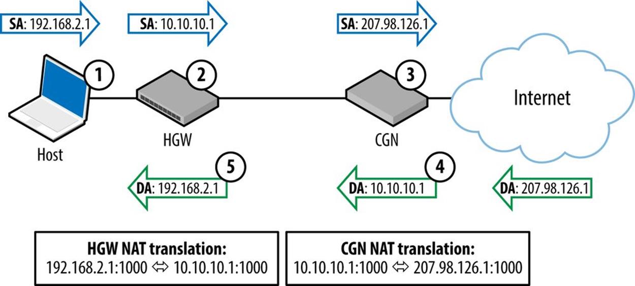
Figure 2-2. CGN (with NAT444) example

Figure 2-2 demonstrates the packet flow for a CGN architecture using NAT444.

The steps are as follows:

1. Host sends packet with private source address (SA).

2. Home Gateway (HGW) changes source address of packet.

3. Carrier-Grade NAT (CGN) maps private to public address.

4. CGN changes destination address (DA) and sends to HGW.

5. HGW changes destination address and sends to host.

The basic CGN/LSN cost-benefit analysis for service providers probes whether or not purchasing additional CGN/LSN hardware (or enhancing existing hardware with CGN/LSN functionality) and developing an operational practice to support CGN/LSN will be cheaper than either immediate or eventual IPv6 adoption.

It’s also not simply a question of cost. Subscriber networks are adding hundreds to thousands of new users every day. To protect revenue, bringing these users online has to be done as quickly and economically as possible. The engineering practice to support such massive provisioning obviously has to be familiar enough to be rapidly scalable.

But you probably won’t be surprised to learn that, like traditional NAT at the enterprise edge, CGN/LSN deployments introduce problems of their own. These issues include:

§ Broken geolocation

§ Difficulty with lawful intercept

§ TCP port-exhaustion

Broken geolocation and reputation services

The maturity of IPv4 means that the IPv4 Internet becomes more like a village (and less like a jungle) with every passing year. Well-established policies and methods exist to track where, and to whom, IPv4 blocks are allocated. Network operators use this geolocation information to measure latency and help optimize traffic delivery. (Content providers and license-holders use the information to make sure that content isn’t delivered to network locations where licensing agreeements haven’t been secured.)

IPv4 reputation services have sprung up to provide the dirt on which networks are sourcing malware, spam, and hacker attacks. This information allows network administrators to block connections originating from IP addresses or ranges known to harbor malicious users.

Because CGN/LSN hides up to many thousands of private addresses behind one or a few public addresses, it can break both geolocation and reputation services.

Lawful intercept

Law enforcement agencies may need to issue requests to ISPs for information regarding Internet users’ activities when those users are suspected of breaking laws. Since CGN/LSN hides user addresses, ISPs deploying it have the burden of tracking transaction data to the port level for thousands upon thousands of NATed sessions. The amount of data generated is voluminous yet must be stored for some period of time to make available to law enforcement upon request, creating additional expense and administrative burden for the ISP.^[52^]

TCP port exhaustion

Many modern Internet-based applications use multiple TCP ports per session. A well-known example of this is Google Maps, where every requested map is subdivided into sections and each map section requires a new TCP port to be opened.

CGN/LSN appliances only have so much memory to track these ports and must share that memory among individual addresses being NATed. Any given host behind a CGN/LSN will thus have a limited number of TCP ports available to them for any particular session. Once these ports are all in use, requests to open new ones must be dropped, which can result in broken applications and degraded user experience (something the content provider, and not the service provider deploying CGN in the first place, may get unfairly blamed for).

Practical Example: Production Loopback Addresses

Managing a bunch of routers is much easier if each router is assigned a loopback address from a single prefix. In IPv4, these addresses are usually /32s assigned from one /24 (or larger prefix), while in IPv6, they are /128s assigned from one /64 (as covered in the section on loopback addresses earlier in this chapter).

A logical numbering scheme can help make it easier for operational staff and processes to track and manage routers. In networks with fewer routers, simple is perhaps best. For example, if the prefix we’ve chosen to use is 2001:db8:aa:90::/64, we could use ::1 as the first address (say for the HQ router) and then number up sequentially from there.

Sequential addresses are, of course, easier for hackers to scan, but we’ll likely have a security policy and set of ACLs in place that isolates our loopback network (while still permitting legitimate device access).

But as we’ll repeatedly demonstrate throughout the book, the abundance of bits available in IPv6 provides the opportunity to encode operational significance into any given address or prefix.

In this case, we have 64 bits to play with, which gives us 16 hexadecimal characters to use for device identification.^[53^]

With 4 bits per character in the address, we could create groups and subgroups that are multiples of (e.g., 16, 256, 4096, or 65536, etc). Note that any hierarchy we create will only be “on paper” and will not be reflected in the actual routing configuration as we’re still just using an entire /64 per routing domain.

Routing domains will often be defined and configured according to geographical regions. This helps segment routing policy in a way that can make it easier to manage network traffic. Returning to our example, let’s say we have a routing domain corresponding to our North American region. We allocate 2001:db8:aa:90::/64 to use for router and device loopback addressing in this region.

We can then examine our logical network topology to look for opportunities to reflect that topology in the loopback addressing.

Let’s say our North American region is divided into three subregions: West, Central, and East. Each region has several core routers interconnecting the enterprise networks of various offices, including the company’s headquarters. There are 30 routers in total. (The routers and switches at each of these locations are managed locally.) The routers are running OSPFv3 as the IPv6 IGP.

As mentioned, we could certainly just number from our /64 sequentially starting at ::1 and number through ::1e. Chances are our existing IPv4 loopback scheme does something similar. By keeping the values the same, we help retain some operational continuity with our IPv4 network.

CAUTION

If you’re planning on using whatever numbering scheme you’re using in IPv4, remember that hexadecimal doesn’t map directly to decimal. In general, we’ll want to avoid IPv6 addressing schemes that restrict us to our existing IPv4 one. We’ll discuss the reasons why in more detail in Chapter 5.

But by doing that we’d be missing the opportunity to encode the geography associated with our topology in our loopback addressing scheme. (This capability becomes especially valuable if we have lots of routers in our core network.)

To illustrate, let’s break our /64 prefix into address groups. First, we’ll look at the range of address values possible for the prefix:

2001:db8:aa:90:0000:0000:0000:0000 - 2001:db8:aa:90:ffff:ffff:ffff:ffff

Next, to keep the addresses tidy, let’s just focus on the last group:

2001:db8:aa:90::[XXXX]/64

Since we already have more than 16 routers in one region, we’ll need more than 4 bits per region. We’d likely want to use more than 4 bits anyway to leave room for the “growth” of our loopback ID scheme.^[54^]

By dividing the last group into 8 bits each, that gives us 256 levels of 256 addresses.

2001:db8:aa:90::[RR][DD]

(Where R represents the region and D represents the device.)

Which gives us:

2001:db8:aa:90::[00-ff][00-ff]/64

The simplest addressing scheme would only require three levels, one for each of our regions, and at least as many addresses as we had regional network devices. In our example, we have 30 total, with, say, 10 routers per region, so the previous address would provide more than enough room for expansion (all the way up to 256 regions with 256 devices per region).

Now we’ll show some actual address-to-device mappings in Table 2-4:

Table 2-4. Address to device mappings

TIP

We certainly could have added one or two bits to increase our available addresses in that group of addresses by 32 or 64 respectively. But recall that we want to stick to using groups of addresses that are always multiples of 2⁴ⁿ so that each character in any given address is significant for the purposes of mapping that address to a particular location.

You might legitimately ask: Isn’t this overkill? Don’t I have DNS to handle the naming of devices? Chances are the great majority of your network management will rely on DNS entries for routers and other devices on the network. First-level operational staff with minimal training certainly will. Senior engineers responsible for building and maintaining the routing configuration will rely on scripts or network management automation tools that use DNS names for devices.

But there are plenty of instances where DNS resolution might fail. Device identification via the IPv6 address protects an additional layer of operational transparency and thus effectiveness. The trade-off between this benefit and whatever additional complexity it entails is a specific instance of the general challenge of balancing the complexity of any operational practice with its general accessibility and extensibility; i.e., if an operational practice is so complex that only a few engineers can learn it and use it, its benefit to the organization may be constricted to only those individuals.

IPV6 AS THE GEOLOGIC AGE OF THE EARTH

Here’s another size comparison between the IPv6 and IPv4 address spaces. According to geologists, the Earth is approximately 4.54 billion years old.

The first humans (the species Homo habilis) appeared on the scene over 2 million years ago. In the figure that follows, that slice of time is just before the very top of the circle.

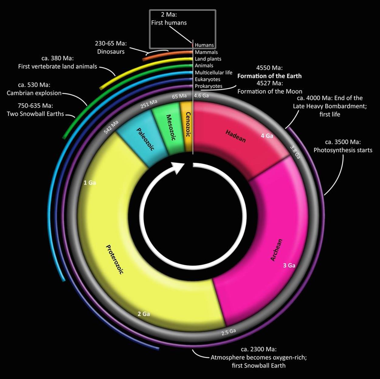
Just to get some sense of how much time that represents in the context of the age of the Earth, let’s calculate the percentage of one arc degree (1°) that 2 million years represents:

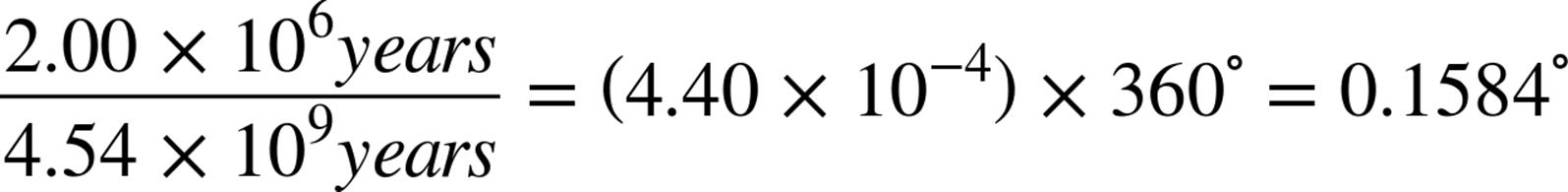
So humans as a genus have been around for nearly 16% of one arc degree (where 360 arc degrees represent the 4.54 billion years the Earth has existed). Modern Homo sapiens are a bright-eyed and bushy-(non)tailed 50,000 years old, or approximately 0.4% of one arc degree in our circle.

For our comparison proper, let’s make that 4.54 billion years equivalent to the total number of IPv6 addresses.

So, how much time would we need to represent all IPv4 addresses?

When I ask this question of audiences during IPv6 presentations, the estimates (by both IPv6 newbies and veterans) are typically in the range of seconds to months.

To find the actual answer, we first divide the number of IPv4 addresses by the number of IPv6 addresses to determine the ratio of IPv4 to IPv6:^[55^]

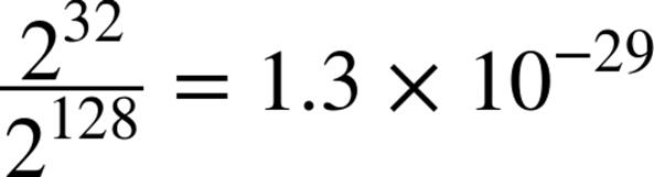
Next, we’ll multiply that ratio by 4.54 billion years (but first let’s reexpress the years as seconds):

Finally:

And we have our answer: Approximately 2 trillionths of a second (or roughly how long it would take light to traverse the period at the end of this sentence).

^[28^] The binary representation is how a computer stores the address in memory and how it appears on the wire.

^[29^] The technically precise (and fortunately seldom-used) term is hexadectet.

^[30^] An alternative recommendation suggests that you should compress the left-most zeros in an effort to keep the network part of the prefix as short and readable as possible.

^[31^] After all, cabs anger faun man…er, anagrams can be fun!

^[32^] One notable exception to this recommendation might include production DNS name server addresses. Such addresses, when memorable, can make any configuration or troubleshooting operations easier to perform.

^[33^] Perhaps this even division of bits suggests the equal importance of global routing efficiency and sufficient host addressing.

^[34^] RFC 4291, IP Version 6 Addressing Architecture. By the way, are you wondering from the table above where the broadcast address type went? If you’re old enough and lucky enough to remember unintentional broadcast storms bringing all LAN traffic to a screeching halt, you’ll be happy to learn that broadcast addresses don’t exist in IPv6. They’ve been replaced entirely with multicast addresses and the much more efficient routing and switching logic they provide.

^[35^] The loopback address has been helpfully described in the standards as “a Link-Local unicast address of a virtual interface to an imaginary link that goes nowhere.”

^[36^] The only instance where this should not occur is if a duplicate Link-Local address is detected on the same segment.

^[37^] While technically the GUA space is everything left once we take out the other address ranges and addresses, only 125 bits (!) of that remaining address space has been allocated for immediate use.

^[38^] RFC 4193, Unique Local IPv6 Unicast Addresses.

^[39^] The algorithm for this is described in RFC 4941, Privacy Extensions for Stateless Address Autoconfiguration in IPv6.

^[40^] PA is sometimes also referred to as Provider Aggregatable space.

^[41^] While these interfaces are usually on different nodes, there’s no rule that says they have to be.

^[42^] RFC 7346, IPv6 Multicast Address Scopes.

^[43^] For example, Google’s public DNS service uses the IPv6 anycast addresses 2001:4860:4860::8888 and 2001:4860:4860::8844 for its name servers.

^[44^] For the example, I’ve used an IPv4 address from the reserved documentation range, but in practice this address must be a globally unique IPv4 unicast address.

^[45^] Keep in mind that you’d still need a DHCPv6 server when using SLAAC to provide any DNS server and domain info to the host. See DHCPv6 Basics for more information.

^[46^] IGP and EGP routing protocols are covered in more detail in Chapter 10.

^[47^] A routing domain can be loosely defined as a collection of routers under one administration and running the same routing protocol instance (e.g., a BGP AS, OSPF process, VRF, etc.). These loopback addresses often correspond to the router IDs used by the routing protocol as part of its route calculation.

^[48^] RFC 6164, Using 127-Bit IPv6 Prefixes on Inter-Router Links.

^[49^] For example, Cisco recently introduced a feature called Destination Guard that explicitly protects an interface from Neighbor Discovery cache exhaustion attacks.

^[50^] RFC 4941, Privacy Extensions for Stateless Address Autoconfiguration in IPv6.

^[51^] RFC 6106, IPv6 Router Advertisement Options for DNS Configuration, proposes including DNS server and search list information in RAs to provide host configuration options for SLAAC currently provided by DHCPv6, but it isn’t widely implemented among host operating systems.

^[52^] The regulations applying to lawful intercept requirements vary by jurisdiction, but in one example, ISPs must keep these data for at least six months. Also, dynamic port assignment and changing port numbers amplify an already staggering data management challenge.

^[53^] Keep in mind that whatever name or function significance we encode into the address using the bits and resulting characters available to us would be separate from whatever DNS entries we might (or might not) create for it.

^[54^] It’s not that we’ll ever run out of IPv6 addresses given that we have 1.8x10¹⁹ at our disposal, but it would be nice to keep our future loopback ID assignments contiguous with the previous per-region ones.

^[55^] Keep this ratio of IPv4 to IPv6 handy if you really want to impress strangers at parties or your in-laws at the next holiday gathering.