IPv6 Address Planning (2015)

Part II. Design

Chapter 5. IPv6 Address Planning Concepts

Practice safe design: use a concept.

— Petrula Vrontikis

Introduction

It’s been said that design is where science and art break even. In this chapter, we’ll focus primarily on the science part of IPv6 address planning and be as thorough as we can be with the design concepts and principles that you’ll need to be familiar with to tackle your plan. As we proceed, however, we’ll be sure to consider the art of address plan design as well, an art based on accumulated operational knowledge and practical experience and the best-practices that have evolved from it.

IPv6 Address Planning Principles

We’ve already mentioned earlier that IPv6 address planning should not be based on (e.g., sufficient host addressing).

But given that, what should it be based on (and why)? Let’s examine the fundamental IPv6 address planning principles in brief before looking at each more closely. They are:

Properly sized initial allocations

This is arguably the most critical of all the address planning principles we’ll discuss. The reason is that all of the principles that follow are more or less dependent on getting a sufficiently large allocation at the start.

Sparse assignment of subnets

With a sufficiently sized allocation, we’ll be able to assign subnets sparsely, i.e., leave unused space between our assigned subnets adequate for future growth or network reconfiguration.

Hierarchical organization of subnets

A sufficiently sized allocation also allows for the organization of subnets into hierarchies or levels that follow one or more organizational attributes of the network or enterprise: geographical location, organizational role, security classification, etc.

Adherence to nibble boundaries

Where practical, assigning subnets based on 4-bit boundaries provides for the operational benefit of increased legibility (i.e., human-readability) for IPv6 subnets.

Uniform subnetting and summarization

Equal-sized subnets (or groups of subnets) help simplify the overall address plan. They’re easier to assign, administer, and track. They’re also easier to summarize, potentially providing for smaller routing tables and tidier ACLs.

Let’s look at each of these principles in more detail.

Properly-Sized Initial IPv6 Allocations

It seems to be an all-too-common occurence for enterprises to end up with an IPv6 allocation that’s too small. A typical example of this is an enterprise that has multiple networks in multiple locations but receives only a single /48. Such scenarios often occur because enterprise network or IT personnel have gotten conflicting, insufficient, or out-of-date information on how much IPv6 space they need, so they end up asking for too little. The absolute enormous scale of a /48 can trigger an analysis that is misinformed by IPv4 thinking: “We’ve got 1,208,925,819,614,629,174,706,176 IPv6 addresses to use. Let’s see…(does calculation)…that’s 281 trillion Internets! But…we don’t want to eventually be in the same boat as we are with IPv4 exhaustion. Better play it safe and figure out how to best carve up our one /48. After all, it’s more than enough host addresses.”^[76^]

So now that we know we’re going to need a properly-sized initial IPv6 allocation, what’s the proper size? Naturally, organizations come in many sizes and have differing missions. Though there are some common allocation sizes by organization type (as depicted in Chapter 3), there typically isn’t a one-size-fits-all allocation. So our more general definition of a proper-sized IPv6 allocation is one that allows for the realization of all the other IPv6 address planning principles. Such principles will help ensure more specific operational benefits like prefix legibility (or human-readability), better route aggregation, more manageable ACLs, and more accurate tracking of IPv6 prefix assignments. The goal is to futureproof the address plan and keep it operationally viable through the growth and change that inevitably occurs in any network.

Of course, attempting to accurately determine how much IPv6 space will be needed before you’ve completed at least an initial version of an address plan means that you may need to make some educated inferences (aka, guesses). Meanwhile, creating an IPv6 address plan relies on knowing how much space you have to work with. As a result, it may be helpful to tackle this sizing conundrum in a couple of stages:

1. By making an initial, approximate estimate based on the relative size of the organization (generally, with regard to the number of sites as uniquely defined in IPv6 terms).

2. Reassessing the estimated allocation size after a detailed plan based on solid IPv6 address planning principles and best-practices has been constructed.

For the first stage, allocations range in size from a /48 at the smallest end (usually for a single site) all the way to a /16, depending on the size of the requesting organization. While there could always be exceptions, ISPs are more likely to receive larger allocations, between a /16 and /32, while enterprises are often allocated between a /48 and /32 of IPv6 space (Figure 5-1).

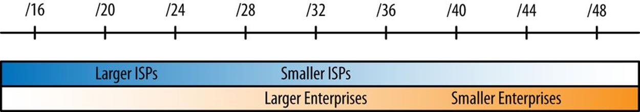
Figure 5-1. Allocation size according to type of organization

We’ll cover RIR and ISP requirements for justifying IPv6 allocations in Chapter 6, but planning on assigning at least a /48 per site is a good rule of thumb for estimating the necessary size of your IPv6 allocation.^[77^]

Also, for those that have already received an allocation from a RIR or ISP: as you create or revise your first plan, you may come to realize or believe that your allocation is insufficient. We’ll cover what to do in that scenario in the next chapter.

Sparse Assignment of Subnets

The next principle of IPv6 address planning is sparse assignment of subnets. We saw a few of the methods for creating subnets that allow for sparse allocation in the previous chapter, such as subnetting from either the left-most or middle bits, either of which leaves additional bits to create additional contiguous subnets in the future.

Hierarchical Organization of Subnets

By grouping subnets into hierarchies (or more simply put, levels), the addressing plan can more closely track the organization of the network: e.g., its physical topology, its security policies, or any other attributes that might make sense to map into the address plan. Each level of the hierarchy should be easy to aggregate into the next level. It follows then that when creating a new level below an existing one, subnets should be equally sized to continue to allow for aggregation. This recommendation is our next principle.

Uniform Subnetting and Summarization

Anytime new subnets are defined for a hierarchy level within an addressing plan, every effort should be made to make sure that they are uniform in size. This requirement makes sense when considered in the context of the previous principle: hierarchy is easier to establish and maintain when using subnets of equal size. This principle also makes for more efficient network operations (and IP address management) when equal-sized subnets are assigned to particular locations or functions in the network. Finally, uniform subnet sizes can help simplify security policies and any resulting ACL entries (reducing the risk of configuration errors).^[78^]

Subnets in Reserve

Getting a big enough block of IPv6 addresses from an RIR or ISP at the outset (as well as using techniques like sparse allocation) should help automatically preserve blocks of subnets sufficient for future use. That said, the principle of holding subnets in reserve should be kept in mind as you develop and iterate your address plan. Having enough subnets in reserve at each layer of hierarchy will help ensure the future flexibility and scalability of the plan.

As the network grows or changes, the ability to maintain the above principles is evidence of a successful addressing plan.

Why Don’t I Use My Existing IPv4 Plan in IPv6?

When getting started with IPv6 address planning, we might be tempted to use an existing IPv4 address plan as a guide or framework. The reasons for this impulse are perfectly understandable. For instance, without the foundation in IPv6 address planning concepts and methods this book seeks to provide, an architect can lack the proper organizing principles with which to build a proper address plan in IPv6. An existing IPv4 plan provides at least some structure (and the concepts and methods that gave rise to it) and seems to offer a manageable entry point into a new planning effort. It’s also already familiar to network administrators.

But there are multiple reasons why this is the wrong approach.

We’ve already discussed some of the common methods resulting from IPv4 thinking. Attempting to somehow correlate our new IPv6 plan with our existing IPv4 one may lead to improper subnetting and summarization.

For example, because IPv4 allocations are often necessarily limited in size, it’s much more common to allocate adjacent subnets. But IPv6 allocations are obviously much larger, and as a result, allocating subnets along boundaries separated by a nibble is the technique preferred in IPv6 address planning. This sparse allocation method leaves intervening bits to number into later, a luxury not afforded to us by the limited bits available in IPv4.

Another reason too much thoughtless deference to our existing IPv4 address plan can be a bad idea is that, unless we’re doing a lot of translation between IPv4 and IPv6, our preferred IPv6 deployment method will be dual-stack. Since the IPv4 and IPv6 networks are logically separate in such an environment, we have the freedom to develop a new and unique address plan for IPv6. The potential benefits of this green-field opportunity cannot be overstated (and are partly the reason this book exists).

A final trap that an existing plan can lay for us is the impulse to map IPv4 addresses into IPv6 addresses for an attempt at operational consistency (with the hopes that it will lead to increased operational efficiency). Some or all of the IPv4 octets could be encoded into the hexadecimal characters of the IPv6 address.

For instance, here’s the IPv4 host address 192.0.2.234 mapped into the last eight nibbles of the IPv6 subnet 2001:db8:777::

2001:db8:777::c000:02ea

You’ll notice that we immediately sacrifice the more familiar decimal representation of the IPv4 address (along with whatever operational benefit it might have otherwise provided). An alternative would be not to convert the decimal characters to hexadecimal, but just represent them using the numbers characters of hexadecimal:

2001:db8:777::192:0:2:234

While this method forgoes any of the benefits of auto-addressing via SLAAC or DHCPv6 (and the tighter host control, DNS, and IPAM potentially available when using it), it might be useful in limited instances where static addressing is usually used, such as specific, well-known servers.^[79^]

Finally, no matter what might be perceived as the immediate operational ease or benefit of mapping our IPv6 address plan into our existing IPv4 one, keep in mind that IPv4 is headed toward legacy protocol status: at some point, organizations will be removing IPv4 from the network. Whatever interim operational benefit was missed out on by commiting to IPv4 address plan logic at the outset, add to that the complexity and expense of revising or redoing the IPv6 address plan according to the established and new best practices.

Address Plan Structure

TIP

At its most basic, the IPv6 addressing plan method is defining and assigning blocks of subnets based on the structure of the network or the organization.

We’ll look at some general best-practice IPv6 address planning principles a little later in the chapter. But first, let’s look at an example of the basic address plan structure (Figure 5-2).

In this example, the level 0 represents an organization’s primary IPv6 allocation from the ISP or RIR. Level 1 represents blocks of subnets defined and assigned to some network or attribute within the organization. Level 2 represents the smallest assignable subnet (in most cases a /64).

More specifically, the example above might correspond to a /48 being carved into 256 /56s, each yielding 256 /64s (or, alternatively, a /32 being carved into 256 /40s, each with 256 /48s). Figure 5-3 shows another example with an additional level added.

As before, level 0 represents an organization’s primary IPv6 allocation from the ISP or RIR. Level 1 represents blocks of subnets defined and assigned to some network or attribute within the organization. Level 2 would be the next block of assigned subnets within each level 1 subnet.Level 3 would likely be the smallest assignable subnet (again, with each instance of level 3 fitting into each level 2 subnet).

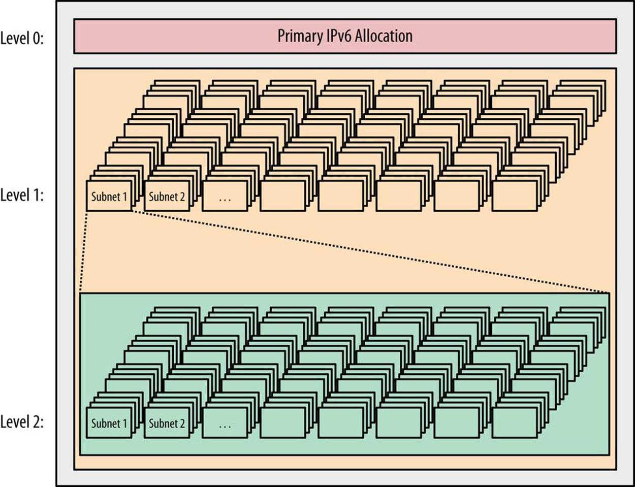
Figure 5-2. Basic address plan structure

As we’ll see in the addressing plan example in Chapter 7, most organizations have fewer than 256 attributes requiring subnet blocks. They also typically have subattributes requiring additional levels. As a result, most address plans end up with many unused subnets in each block (Figure 5-4).^[80^]

When we talk about blocks of subnets defined and assigned to a level, each level typically corresponds to some well-defined network or organizational attribute, and the most significant of these (and typically the first to be defined) is the site.

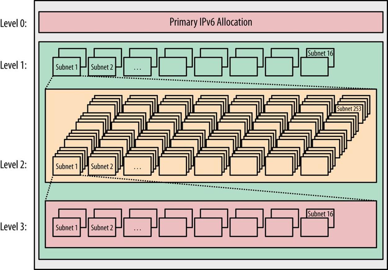
Figure 5-3. Basic address plan structure

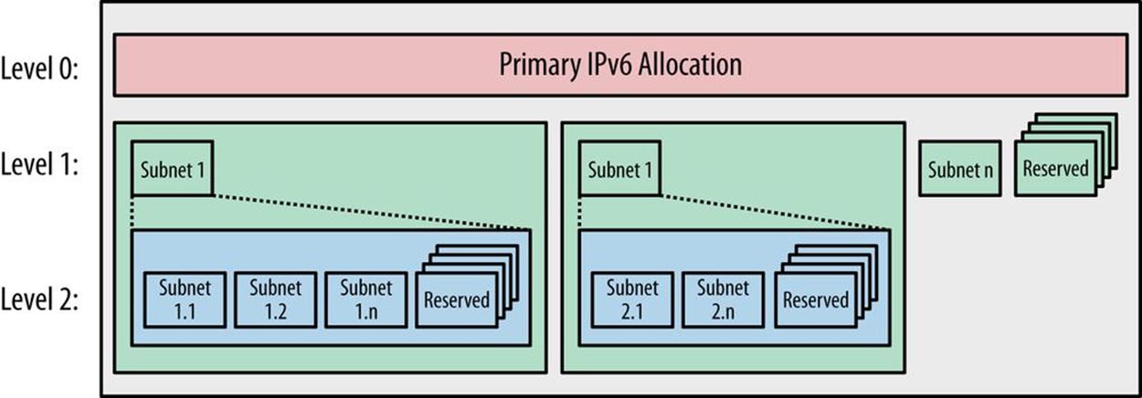
Figure 5-4. Address plan structure with reserved (unused) subnets

What Is a Site?

We should already have some concept of what constitutes a site when it comes to general network architecture and addressing. Since the network exists to provide services to the organization, a site is very often defined by its generic role: e.g., headquarters, remote office, research campus, home network, data center, point-of-presence, etc. Often, these designations are prepended with actual geograhical locations: e.g., Atlanta HQ, Fresno remote office, Frankfurt POP, etc.

We also might think of sites more abstractly: e.g., as discrete LANs behind routing aggregation points, IGP areas, security domains, etc.

NOTE

In the context of IPv6 address planning, it can be helpful to think of a site as a fundamental network (or organizational) unit that receives a uniform network prefix. Keep in mind that we shouldn’t define a site in a way that prevents us from realizing our basic address planning principles (an outcome that is more likely if we have defined too few or too many levels of hierarchy).

Thus, our choice of how we define a site within our network or organization will have a critical impact on our IPv6 address plan; specifically, how much IPv6 address space we should request from an RIR or ISP (and can reasonably expect to receive).

A little bit of background on the subject should help provide some helpful context for this process.

In the early days of IPv6 adoption, members of the IETF wanted to create some useful guidelines for allocating IPv6. As a result, way back in 2001, the Internet advisory board (IAB) recommended that the allocation for “the boundary between the public and the private topology” be a /48, except “for very large subscribers.”^[81^]

As we’ve covered, such an allocation left 16 bits available for additional subnetting before reaching the /64 host ID boundary and was seen as a good balance in size for small and large enterprises, as well as home networks.

A fixed /48 allocation size for all sites offered a number of operational and administrative benefits for both the allocating agency and the recipient.

For an RIR or ISP, a fixed allocation meant they didn’t have to worry too much about whether requests were appropriately sized or know too many of the gory details of the recipient’s network or plans for growth. A fixed allocation of sufficient size could prevent the recipient from having to come back for additional space any time soon after the initial allocation, a potential boon to both the end-user and the RIR or ISP.

For the recipient, benefits included things like the relative ease of renumbering (should it be required). With a fixed allocation size for sites, any new allocation would have the same number of bits in the network portion of the address, making renumbering much simpler. Another benefit would be being able to use and manage one reverse DNS zone per site. And perhaps most compelling of all (at least for our discussion) is that a fixed /48 allocation size made address planning and management much simpler and more consistent.

At the time, the issue of conservation was considered. Would a /48 allocation for all sites create premature scarcity in IPv6 overall (i.e., shortages within the address protocol that was designed explicity to overcome a scarcity problem in the first place).

The answer was a resounding no. The 35 trillion available /48s in the existing global unicast allocation were deemed sufficient (and with approximately 87% of the total IPv6 address space remaining unallocated, any misjudgements or miscalculations on this question would be easily absorbed by a newly defined GUA, potentially one with tighter allocation policies).

IN THE YEAR 2100 CE

Perhaps it’s time for another demonstration of the sheer magnitude of the IPv6 address space.^[82^]

The current global unicast allocation 2000::/3 is defined by the three highest-order bits of the 128-bit address being set to 001. A little arithmetic reveals that this allocation is 12.5% of the overall IPv6 address space:

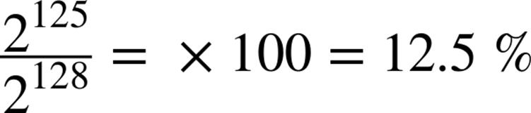
Next, we’ll calculate the number of /48s in the GUA. This quantity can be easily determined by subtracting the number of bits defining the network portion of the GUA (indicated by the /3 of its CIDR notation) from the number of bits defining the network portion of the site allocation (indicated by the /48 of its CIDR): e.g., 48 - 3 = 45. Thus, there are 2^45 /48s in the GUA.

35,184,372,088,832

The UN predicts that by 2100 the Earth could have a human population of as many as 16 billion people. Will posterity have enough IPv6?

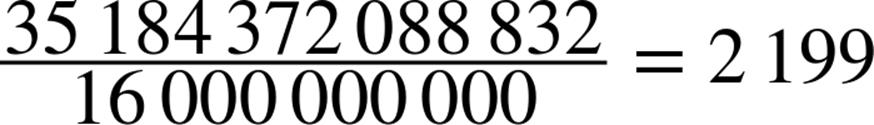
So even with a potential population of 16 billion, there are still enough /48s in the GUA to provide every person on Earth with almost 2,200 of them (and that’s with approximately 86% of the IPv6 space still held in reserve).

Based on these numbers, the argument goes that over the next 80 years IP will, in all likelihood, be superseded by other communications protocols.

Since then, the recommendations have been updated to allow for subnets smaller than a /48 (e.g., /56) to be assigned to sites.^[83^] This was done less out of any concern for the potential to “waste” IPv6 space and more as a recognition that some operators would want the flexibility to use a smaller assignment to make their plan more operationally manageable. In particular, broadband service providers might want to assign more than a /64 to CPE devices inferring that future home networks will need additional subnets to support new services (without perhaps requiring the 65,536 /64s provided by an entire /48).

Of course, the individual sites in our plan could also require an IPv6 allocation larger than a /48. As we develop our plan according to the concepts and principles within this chapter, it’s perfectly acceptable to conclude that a /48 per site would be insufficient to realize the benefits of an IPv6 address plan. RIR policies for IPv6 are still evolving, but a well-designed plan that maximizes operational benefit for the requestor and hastens the overall deployment of IPv6 should be favorably viewed and accommodated, even if said plan requires more than a /48 per site.

Intra-Site Versus Inter-Site Planning

Because of the suggested subnet size for sites (/48) and for interfaces (/64), there is a certain amount of structure already implied for any addressing plan.

In most IPv6 addressing plans, this structure is applied geographically, i.e., to network or organizational topology.

If we think about the 16 bits between a /48 and a /64 prefix as most generally being reserved for intra-site addressing (i.e., subnets within sites), and the 16 bits between a /48 and a /32 prefix as generally reserved for inter-site addressing (i.e., subnets between sites), we’ve identified a basic structure that can help organize our initial effort (Figure 5-5).^[84^]

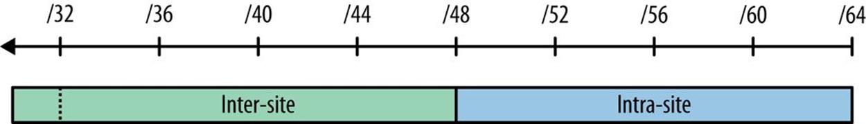
Figure 5-5. Inter-site and intra-site planning

Recall that the standards and RIR policies provide a very broad definition of what a site can be. As a result, an organization has tremendous latitude to assign site designations. Such flexibility is beneficial because there may be multiple site types, each with potentially differing topologies.

In the last chapter, we saw Figure 4-1, which demonstrated eight possible hierarchies (created by choosing different nibble-aligned combinations of the available 16 bits) that we could use for a site’s IPv6 address plan. These hiearchies can be mixed and matched to create unique intra-site address plans for groups of sites that share the same organizational or network topology. An organization might need a small library of address plan templates for when new sites of any type are to be added.

While multiple types of sites could exist (with variations on the intra-site address plan for each type of site), it’s more desirable to attempt to keep the address plan uniform for all sites. In any case, for most enterprises there is typically only one topology between sites.^[85^] As a result, only one inter-site address plan is usually needed. (Although as with the intra-site address plan, variations of the inter-site plan based on regional or architectural differences might be necessary or desirable.)

AS, REGION, SITE

A common way to structure the inter-site part of an address plan is based on a hierarchical network topology corresponding to an autonomous system (AS), regions, and sites (Figure 5-6).

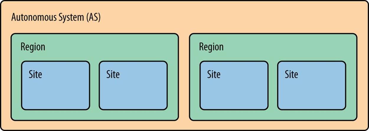
Figure 5-6. Inter-site structure using AS/Region/Site

Typically, the entire IPv6 allocation would be assigned to the AS. An AS is “a set of routers under a single technical administration”^[86^] and with one or more interior gateway protocols (IGPs) providing routing within the AS. An exterior gateway protocol (EGP) — usually Border Gateway Protocol (BGP) — provides routing to other external autonomous systems.^[87^]

The next level of the topology for the inter-site part of our address plan is generally based on regions. The initial allocation is carved up into prefixes of equal size, which are then assigned to specific geographical regions. Regions might be global, continental, national — any designation that works for the organization.

Finally, each of those assignments are themselves divided equally among the sites within the region.

Here’s a more specific example of how a large US enterprise might apply this concept (Figure 5-7):

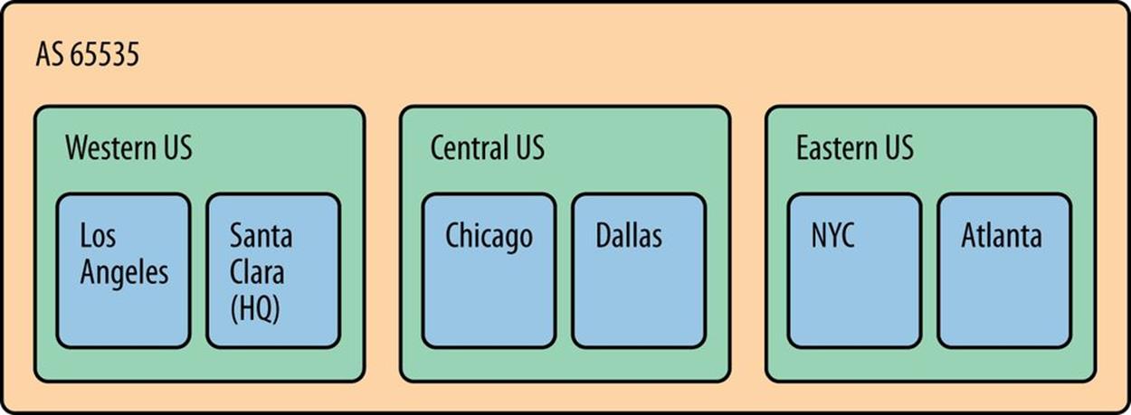
Figure 5-7. Inter-site structure large US enterprise

TIP

For many organizations, especially those with very simple network topologies and operational requirements, this basic division is sufficient for coming up with a workable address plan.

But for everyone else, some additional structure will be required. Here’s the general address plan process:

1. Obtain a primary IPv6 allocation.

2. Identify or define the organizing attributes and hierarchy of the network or the business (e.g., geographical location, organizational role, security classification, etc.).

3. Assign blocks of subnets within each attribute or hierarchical level to satisfy their immediate and future subnet requirements.

Another way of conceiving of this approach is that it is a top-down, compared to the bottom-up, approach in IPv4 relying on host counts.

As we covered in the last chapter, by adhering to the nibble boundary when allocating bits for subnets within a site or between sites, a limited structure or hierarchy can be achieved. Of course, we’re not restricted to only using 4-bit boundaries.

In fact, we can represent in our addressing plan as many branches and sub-branches as we like to correlate to network function, location, names of US presidents, etc. But we need to keep in mind that the more levels we create, the more complex our plan becomes, and the less flexible and scalable it potentially gets. That’s why we should learn and keep in mind some general, best-practice principles.

IPv6 Allocation Methods

When you’re putting together your initial IPv6 addressing plan, you’ll obviously need to allocate subnets to the various entities you’ve defined (e.g., regions, sites, buildings, applications, VLANs, etc.).

When we talk about IPv6 address allocation methods, we’re really talking about the same basic technique that we use in IPv4, i.e., designating bits to define subnets for assignment. The minor technical difference, of course, is that rather than converting from binary to decimal as we did with IPv4, we’re converting from binary to hexadecimal.

But we’re still dealing with the basic process of bit math and subnet definition that we’re already intimately familiar with from IPv4. As a result, the same allocation methods we use in IPv4 are available to us in IPv6.

Besides the minor technical difference mentioned above, there’s a major conceptual difference in how we perform IPv6 address allocations. With IPv6, we’re allocating from abundance rather than from the scarcity of IPv4.

Let’s review the IPv6 allocation methods at our disposal:

§ Best-fit

§ Sparse

§ N+1

§ Random

Best-Fit Allocation

Best-fit allocation usually refers to the following method:

1. Find the smallest unassigned block in the overall address space that the request fits in.

2. If possible, successively halve that block until the smallest block that will meet the needs of the request is defined.

3. Allocate this block.

First, an example from IPv4: say a data center required 375 IPv4 addresses in the same subnet to assign to servers. The organization is using 10.0.0.0/8 as its overall allocation, and the subnet 10.10.0.0/16 has just been assigned to the region that the data center is in. Using the best-fit method, we don’t have to think too hard about the first step because no space has been assigned from this allocation yet. Proceeding to the second step, we halve the original allocation and halve each resulting half until we reach the smallest block that will accommodate the request; in this case, a /23 for 512 total addresses, 375 of which are right around 75% utilization. A pie graph is helpful in visualizing this process (Figure 5-8).

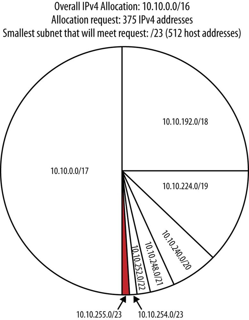
Figure 5-8. IPv4 best-fit allocation example

This result and the method behind it might typically be considered the “most efficient” in terms of IPv4 allocation. But keep in mind that such efficiency is defined as maximum utilization of the IPv4 host addresses available within the smallest assignable subnet, and therefore, is primarily about host address (and subnets for host address) conservation (i.e., IPv4 thinking).

If future allocation requests are of a similar size, it may be possible to consistently use adjacent subnets as you allocate. This, too, will result in more of the available space being “filled in” (i.e., a more thorough utilization of scarce IPv4).

More likely, allocation requests competing for the same overall address space will arrive at different times from different segments or functions in the network topology. The best-fit method pretty much ensures that the resulting discontiguous subnets will be very difficult to summarize for purposes of routing aggregation or access-list (ACL) manageability.

The basic method of best-fit allocation is the same in IPv6, but instead of host address requirements, the allocated block provides the number of subnets needed for a particular assignment.

For example, if the data center from our first example has 375 VLANs that it needs /64s for, the smallest block that will accommodate the request is a /55 (Figure 5-9):

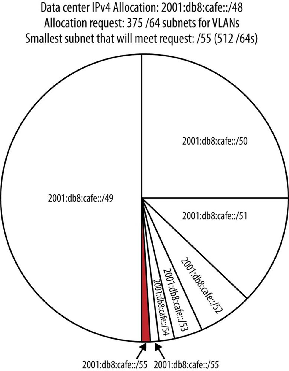
Figure 5-9. IPv6 best-fit example

Though in IPv6 we’re defining and allocating a block to provide subnets instead of individual host addresses, the logic of the best-fit allocation method is still about “right-sizing” the block to use. Later, when our plan is operational and we’re allocating blocks based on changing requests, the subnet size requirements will vary, depending on the number of elements the requestor needs subnets for.

As a result, best-fit allocation is typically a poor first choice when designing an initial address plan.

Sparse Allocation

As you might have guessed, sparse allocation is about leaving a lot of space in between allocations. Sparse allocation is sometimes referred to as bisection. And though it shares the successive halving process with the best-fit allocation method, the sparse approach allocates the block at the edge of each new half.

Figure 5-10 depicts sparse allocation of /52s using a pie chart. In this example, only the 1st, 5th, 9th, and 13th /52s are allocated, while the remaining space between allocations is held in reserve for future use.

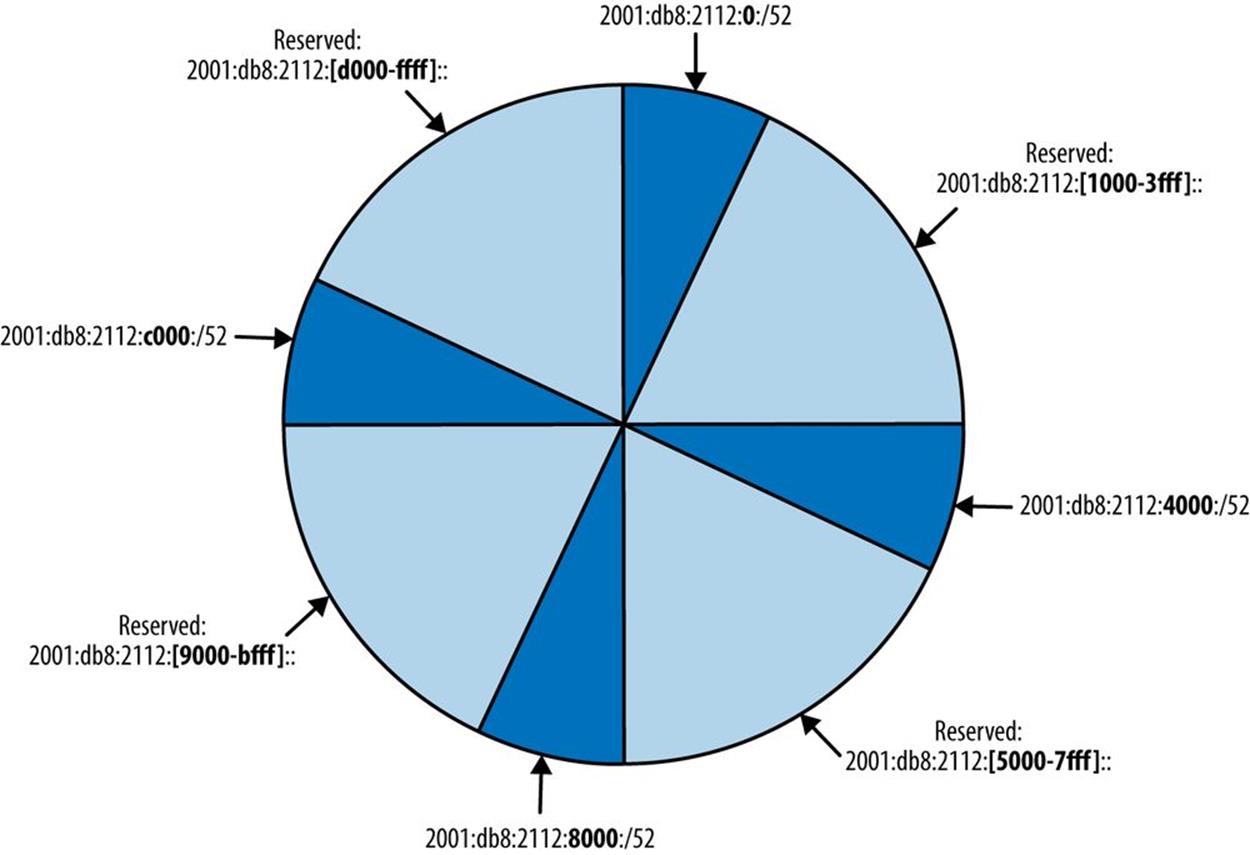
Figure 5-10. Sparse allocation of /52 subnets

Figure 5-11 depicts sparse allocation of /56s using a pie chart. In this example, only the 1st, 64th, 128th, and 192nd /56s are allocated, while the remaining space between allocations is held in reserve for future use.

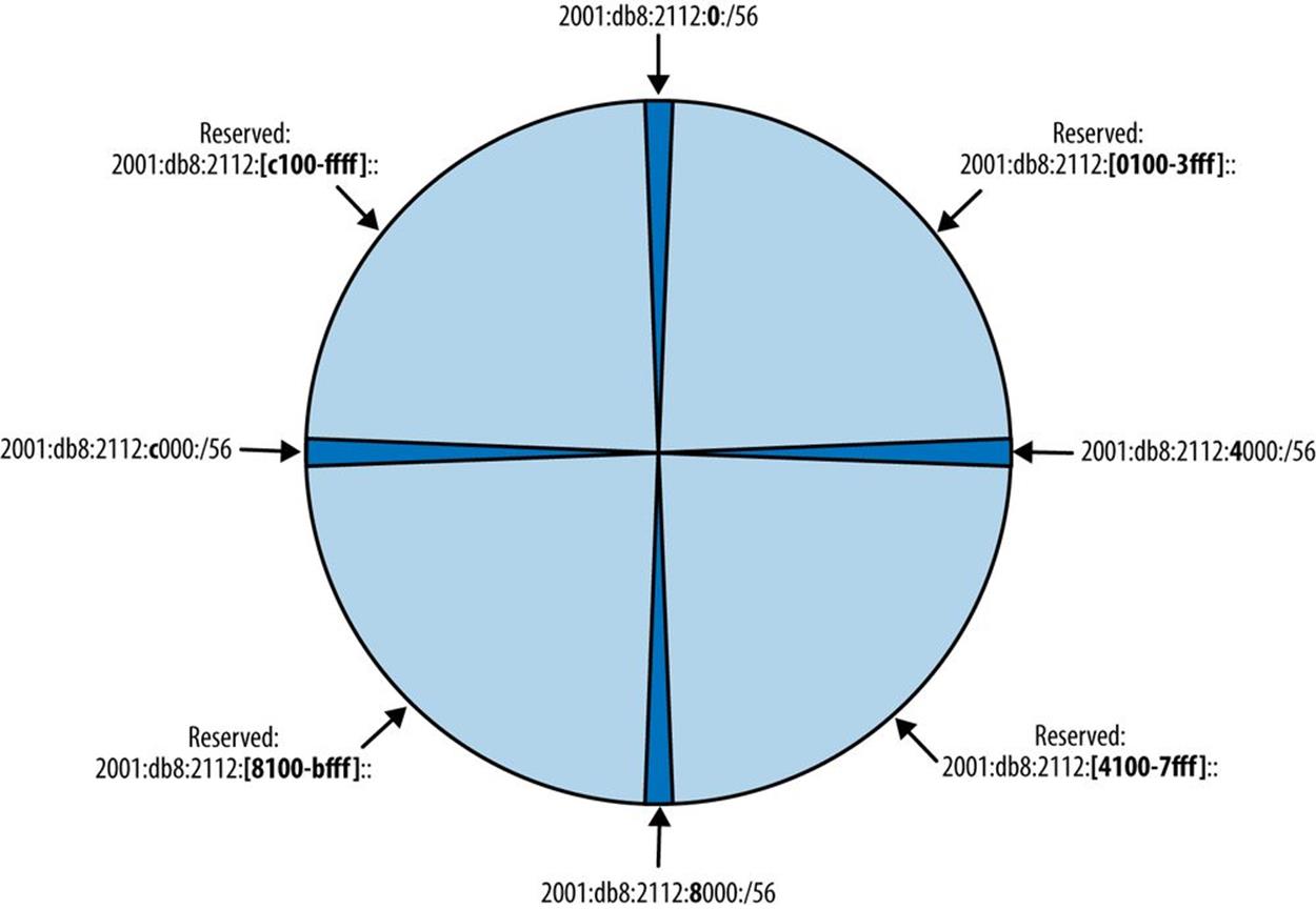
Figure 5-11. Sparse allocation of /56 subnets

Recall the subnetting method from Chapter 4 in which we created subnets by starting with and incrementing the left-most bits.

Let’s use the same site allocation from the above best-fit example:

2001:db8:2112::/48

We can safely ignore the first three hextets of the network ID and focus on the bits of the fourth hextet:

0000 0000 0000 0000

Next we’ll modify our best-fit example a little and say that we have 20 buildings at our site. The minimum number of bits we’d need to provide allocations for all 20 buildings would be 5 (2⁵ = 32).

But recall also from the previous chapter the advanatage of adhering to the nibble boundary. Rounding to 8 bits give us:

2⁴⁽ⁿ⁾ (where n=8) = 256 possible subnets

Since we’re using 8 of the sixteen available bits for our fourth hextet, the resulting network length will be /56. As a result, we don’t care about the right-most eight bits:

0000 0000 XXXX XXXX

The next step would be to begin with the remaining left-most bits and increment bitwise (Table 5-1):

Table 5-1. Sparse allocation example

Now we’ll look at how these subnets increment graphically. But because we don’t want our graphic to become too cluttered, we’ll focus on the first 10 entries in the table to establish the sparse allocation pattern (Figure 5-12).

Between Figure 5-12 and Table 5-1, you may observe that the subnets increment in a way that corresponds to a new allocation at the edge of each new half of the available space.

One of the key advantages of creating an IPv6 address plan from scratch is that you can plan equal-sized address blocks for levels of hierarchy in the network. These equal-sized blocks can then be sparsely allocated, leaving room for growth between allocations and allowing for easieraggregation and ACL maintenance. As a result, the sparse allocation method is typically the most appropriate one to use when creating a new IPv6 addressing plan.

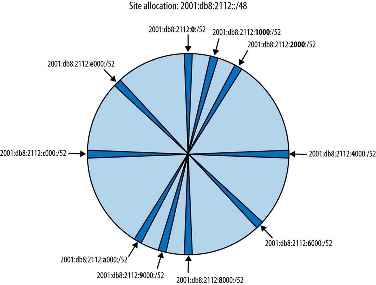
Figure 5-12. Sparse allocation of /56 subnets

NOTE

One variation of the sparse allocation method is referred to as growth-based. In this method, the unused space contiguous with the slowest growing allocation is selected next to be halved again to generate a new subnet allocation. This approach is arguably more useful in service provider environments where allocations may go to different customers and be under independent control. (It conserves the maximum amount of contiguous space for faster growing customers.)

N+1 Allocation

N+1 allocation (which could also be referred to as sequential, or strict sequential allocation) is pretty much what it sounds like: a larger allocation is divided evenly among smaller subnets that are assigned in numerical order. As a result, there is no space between subnets to accommodate future growth for any of the assignments. Any original assignment that required additional space (except the most recent assignment) would necessarily receive a noncontiguous new subnet.

N + 1 VERSUS SPARSE ALLOCATION

For this discussion, N + 1 allocation is a method for a strict sequential allocation of subnets within a site (or for the entire IPv6 allocation), where N is equal to the hexadecimal value of the allocation immediately prior to the one being allocated.

Let’s look at an example of this approach.

Recall that a /48 gives us 65,536 /64 networks. Given that each of these subnets has 1.8x10¹⁹ addresses, we certainly have enough to allow us to simply begin to assign /64 networks in a sequential fashion without worrying about running out of addresses.

2001:db8:1100::/64 Subnet 1

2001:db8:1100:1::/64 Subnet 2

2001:db8:1100:2::/64 Subnet 3

...

2001:db8:1100:ffff::/64 Subnet 65536

There are some glaring deficiencies with such a method.

First, unless our network never changes after our initial address allocation, we’re obviously going to need to assign additional subnets. If we’re merely grabbing the next available subnet in our list, there’s no guarantee that this subnet will be needed for the same physical or logical area of the network as the subnet before it or after it.

As a result, over time, subnets that should otherwise be grouped together for the same location or function in the network become sporadic and disconnected with less efficient ways to logically associate them with each other for management purposes. Also, if a particular network location or function requires a contiguous block of prefixes, it may be necessary to allocate a previously unused block.

In the typical hierarchical network topology, these discontiguous networks mean that our routing tables are larger than they have to be, with many /64 prefixes routed to disparate network locations that would otherwise be aggregated. Larger routing tables slow down convergence times and require more router memory. The potential results are a slower and more expensive network.

From a security standpoint, such discontiguous networks also require more effort to maintain secure access to using ACLs. Single prefixes can result in longer ACLs, which become more prone to configuration errors. Abandoned and out-of-date ACL entries can lead to costly security breaches. Security policies in hardware and software that assume logical groupings of network prefixes according to business roles and compliance rules can become unnecessarily complex or even unenforcable.

Limited or no correlation of business or administrative logic to summarized groups of network prefixes means that it becomes harder and more costly to operate the network. Any single prefix could potentially belong to any location or function and additional context may be required to isolate and effectively troubleshoot hosts or services addressed with it (or otherwise relying on it). Operational costs for troubleshooting are increased.

Sporadic and discontiguous assignment of subnets can increase the cost and difficulty of maintaining the address plan itself, especially in the absence of specialized IP address management (IPAM) systems that allow dynamic representation of the network prefixes and addresses.

By comparison, sparse allocation of network prefixes within an IPv6 address plan can prevent the above issues. It helps provide:

§ Sufficient, contiguous IP space in reserve for future growth

§ Well-defined and stable boundaries leading to more efficient routing and easier management of security policy and associated ACLs

§ A better basis for correlating the topology of the network to the structure of the organization

§ Easier network operation and troubleshooting

§ Cleaner, tidier, and more error-free creation and administration of the plan itself

Finally, keep in mind that within sparsely allocated subnet groups themselves, N + 1 allocation is not necessarily problematic. In fact, allocating the next available subnet is often the preferred method of assigning /64s within a larger sparse allocation.

Random Allocation

Random allocation also divides a parent allocation evenly among smaller subnets, but as compared with N+1 allocation, assigns them not in order but rather in a random fashion. Such a method may be of use where assignments are more dynamic since it could be used to provide a minimal layer of security by obscuring assignment logic (as compared with any of the other allocation techniques). While this method increases the probability that a contiguous subnet would be available for growing a previous assignment, we’ll go ahead and infer that any deployment utilizing this approach isn’t too concerned with summarization or ACL manageability.

Assigning Subnets by Location or Function

Two of the most common organizational attributes used to define and assign subnets within a site are location and function.

Location, as the name implies, is usually physical in nature and corresponds to an actual geographical location within the organization that contains some part of the network: e.g., buildings, floors, IDFs (if you’re into old-school telco jargon), etc.

Functions, meanwhile, can be any logical or administrative entity and are often associated with some specific set of users (e.g., students, guests), hosts (e.g., mobile devices), servers (e.g., development, finance), or roles (e.g., accounting, engineering).

Either function or location significance assigned within a site prefix can be generalized and kept consistent across multiple sites for maximum operational consistency and efficiency, even as the site prefix changes.

Let’s look at assigning location signifcance to subnets created from a sample site prefix. Here’s a generic site assignment:

2001:db8:2112::/48

As we reviewed in Chapter 4, we can create subnets and groups of subnets using any of the 16 bits available to us from /48 to /64. The Xs in the brackets of the fourth hextet represent binary bits:

2001:db8:2112:[XXXXXXXXXXXXXXXX]::

Recall also that adherence to the nibble boundary when defining subnets helps keep resulting address prefixes readable (also, consistently sized, easy to aggregate, and more operationally manageable, etc.):

2001:db8:2112:[XXXX XXXX XXXX XXXX]::

Choosing to adhere to the nibble boundary also reduces the number of available hierarchy levels, which can greatly simplify our address planning. The only requirement is that this simplifed hierarchy needs to fit the underlying network topology or organizational structure.

Let’s give the first nibble location significance:

2001:db8:2112:[LLLL XXXX XXXX XXXX]::

This creates 16 /52 subnets. Expressed in hexadecimal (where Us represent unused hexadecimal characters):

2001:db8:2112:[0-f]UUU::/52

So, in this case, the first level of hierarchy for a site would be 16 /52 subnets that we’ve assigned location significance; e.g., say we’re creating an address plan for a campus with fewer than 16 buildings (Figure 5-13).^[88^]

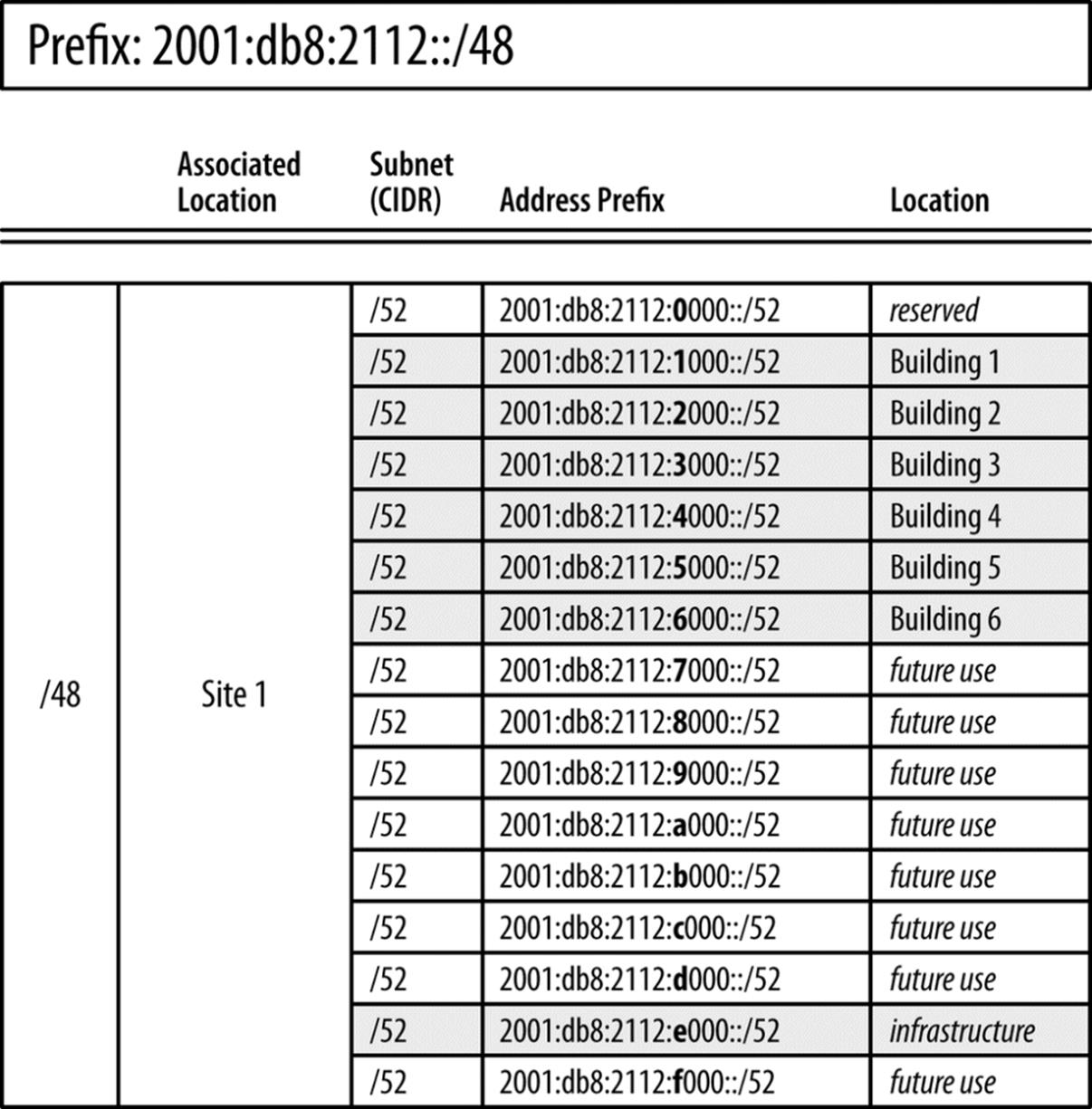
Figure 5-13. 16 /52s, Location significance in first nibble

12 bits remain to assign to additional locations (or 3 nibbles to keep the example consistent).

Recall that groups of subnets assigned a location are often defined to correspond to a point of aggregation within the network. And, of course, we’re not limited to location in assigning any of the next nibbles. Functional assignments for groups of subnets often correspond to security policy and ACL entries.

With that in mind, we’ll give the next nibble functional significance:

2001:db8:2112:[LLLL FFFF XXXX XXXX]::

This creates 16 /56 subnets:

2001:db8:2112:L[0-f]UU::/56

L represents the location subnets, while Us still represents unused hexadecimal characters.

So now we have 16 /52 subnets for each network location, each with 16 /56 subnets that can be assigned to network function (Figure 5-14).

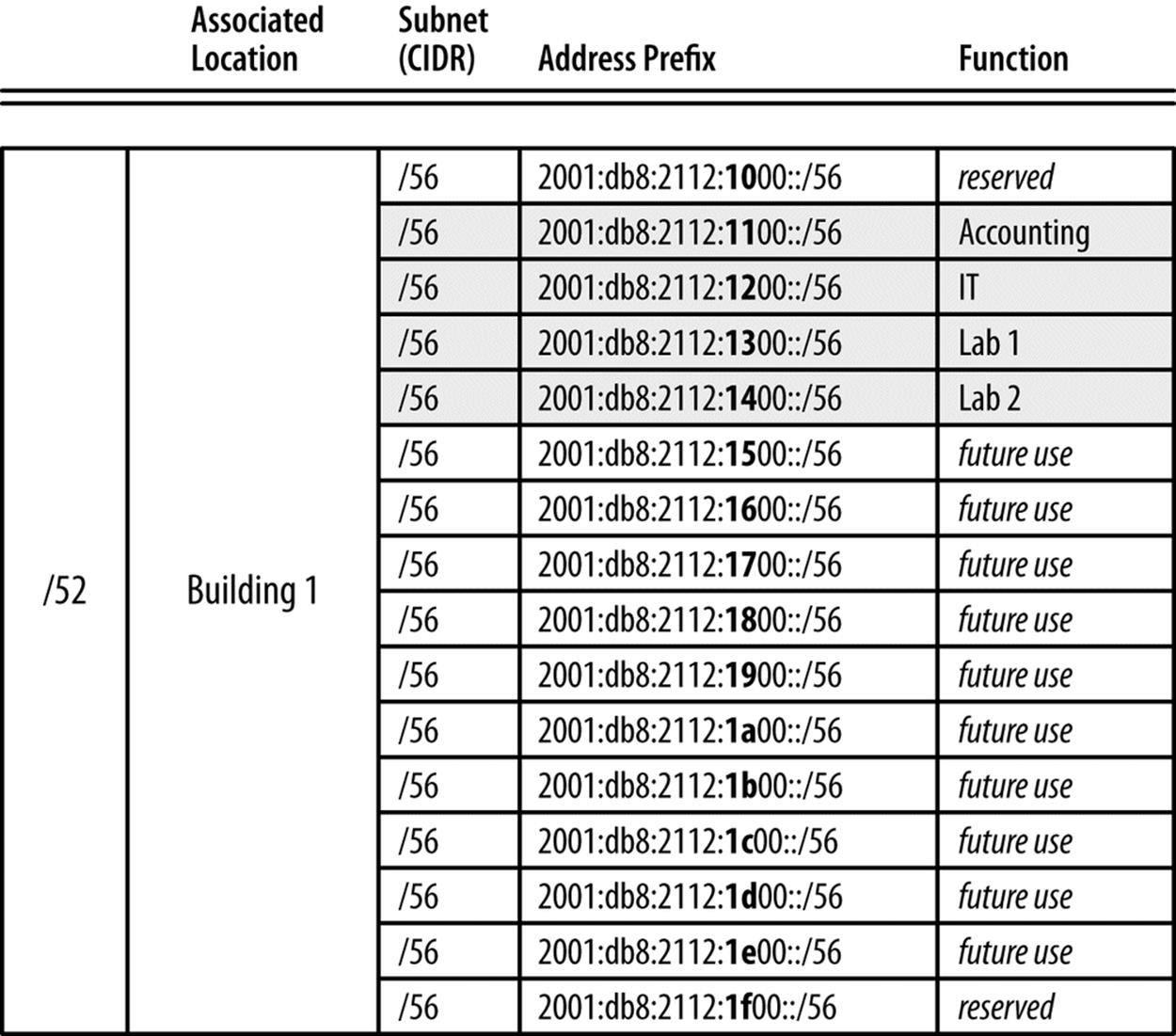
Figure 5-14. 16 /56s, Function significance in second nibble

In the example above, we’ve selected four functions (Accounting, IT, Lab 1, and Lab 2) that correspond to groups of hosts sharing a particular security policy. Administration of their associated ACL entries is greatly simplified by each function’s well-defined (and human-readable) prefix.

At this point, we could use the 256 /64s in each /56 for individual router or switch segment interface assignments.

2001:db8:2112:LF[0-f][0-f]::/64

You may recall that this progressive allocation of bits along the nibble boundary corresponds to one of the paths in the IPv6 site visualization example from Chapter 4 (Figure 4-2).

Note also that we’ve held the first subnet (2001:db8:2112:1000::/56) and last subnet (2001:db8:2112:1f00::/56) in reserve. There are two reasons for this.

The first reason applies only to the first subnet (and its equivalent in other subnet groups). It’s explained in greater detail in Zero Subnets Have a Problem, but to briefly summarize: any subnet uniquely identified by a zero can cause confusion for operational personnel. It’s common sense to want to identify the first subnet in any group with the number 1 (as opposed to 0).

The second is that, whatever other subnets we might hold in reserve for future use, we have at least two “last-resort” subnets reserved at this level of hierarchy.

VLAN-Mapped IPv6 Addresses

While it’s generally not recommended to tie the IPv6 addressing plan to the existing IPv4 one, some network administrators have historically found it beneficial to map VLAN numbers into IPv4 addresses.

This practice is even easier to accommodate in IPv6, given the much larger standard prefix assignment sizes and the additional bits available to represent and encode information like VLAN numbers.

The easiest method to accomplish this is to simply use decimal values in the address to represent the VLAN. For example, say a site receives the standard /48 assignment:

2001:db8:b0b0::/48

Our example site has a few dozen VLANs defined and configured. Because of changes to the network over time, these VLANs are not contiguous and are not consistently numbered but range in value from VLAN 2 up to VLAN 3030. Here’s a small sample of the VLANs in use:

VLAN 2

VLAN 5

VLAN 10

VLAN 12

VLAN 200

VLAN 210

VLAN 1501

VLAN 3030

Using the four characters of the fourth hextet allows us to easily map these VLANs into our site assignment prefix:

2001:db8:b0b0:2::/64

2001:db8:b0b0:5::/64

2001:db8:b0b0:10::/64

2001:db8:b0b0:12::/64

2001:db8:b0b0:200::/64

2001:db8:b0b0:210::/64

2001:db8:b0b0:1501::/64

2001:db8:b0b0:3030::/64

This simple method makes it easy to track and troubleshoot VLANs and their associated address ranges. But you may observe that since these are actually hexadecimal values being interpreted as decimal, the associated subnets are distributed piecemeal throughout the overall assignment. Look at the distribution of bits within the fourth hextet (Table 5-2):

Table 5-2. VLAN hex-as-decimal values into binary

This distribution of bits prevents easy summarization or subnetting of the remaining address space. If the site is relatively small and topologically flat (and likely to remain that way indefinitely), the simplicity and operational benefit of this method may offset any resulting liability.

But most sites will have at least some network hierarchy or other logical structure that makes it beneficial to preserve some bits to use for consistent summarization or subnetting.

This can be accomplished by converting VLAN decimal values to hexadecimal (Table 5-3):

Table 5-3. VLAN decimal values into hexadecimal

Since the maximum number of VLANs is 4,096, all possible VLAN values can be represented with 12 bits. Here’s how the original addresses would be expressed hexadecimally:

2001:db8:b0b0:2::/64

2001:db8:b0b0:5::/64

2001:db8:b0b0:a::/64

2001:db8:b0b0:c::/64

2001:db8:b0b0:c8::/64

2001:db8:b0b0:d2::/64

2001:db8:b0b0:5dd::/64

2001:db8:b0b0:bd6::/64

With this configuration, 4 bits remain for a total of 15 additional subnets (each with up to 4,096 VLANs):

2001:db8:b0b0:[1-f]XXX::/52

Using this method, some of the immediate operational benefit is arguably lessened: operations personnel would now need to first convert hexadecimal into decimal before correlating a given subnet with its associated VLAN. However, the architectural benefit of reserving at least some subnets for additional assignments will make the trade-off worthwhile for most planners.

Summary

When the proper concepts are understood and the right principles are applied, IPv6 offers the opportunity to create an address plan that is scalable, flexible, extensible, manageable, and durable far beyond what is possible with IPv4 networks. Moreover, the operational benefits of a proper plan extend beyond the simple, effective management of the IPv6 prefixes themselves. The ability to encode network location and function in prefixes provides another layer of useful data for effective identification, isolation, and troubleshooting of network issues.

The basic method in IPv6 address planning of defining and assigning blocks of subnets based on the structure of the network or the organization moves us away from the IPv4 thinking that obliged us to consider scarcity and waste and to allocate addresses and prefixes primarily on the basis of host conservation. There are certainly risks of too much deference to our existing IPv4 address plan and allocation, especially considering that IPv4 will soon become the legacy protocol.

A broad and flexible definition of what constitutes a site along with inter-site and intra-site planning concepts provides a simple but powerful framework to apply to our own address plans and the networks they serve. These also allow for the attainment of the address planning principles that will ensure that our plan endures through the inevitable growth and change of our respective organizations and networks. These principles include properly sized initial allocations, sparse assignment of subnets, hierarchical organization of subnets, adherence to nibble boundaries where practical, and uniform subnetting and summarization.

^[76^] While it’s certainly theoretically possible to receive too much IPv6 space, any conclusion that too much space has been allocated needs to be scrutinized through a careful assessment of the proposed IPv6 address plan. Such an assessment should focus on the operational viability of the plan. In other words, does it make network operations over time easier rather than harder?

^[77^] Recall that a site in IPv6 is a logical concept and can apply to any consistently defined network, location, function, etc.

^[78^] Note that this principle has been reflected in the IPv6 standards suggesting /48 site prefixes and /64 interface prefixes.

^[79^] Though I’ve used the IPv4 and IPv6 documentation prefixes for the example above, in an actual production configuration, the mapped address would be constructed from globally unique (i.e., public) addresses.

^[80^] Recall that this is an ideal outcome according to the general principle of Subnets in Reserve we covered earlier in the chapter.

^[81^] RFC 6177, IPv6 Address Assignment to End Sites.

^[82^] This one is courtesy of IPv6 solutions manager, Cisco Press and Network World author Jeff Doyle (CCIE #1919).

^[83^] RFC 6177.

^[84^] If your IPv6 address plan is for a large service provider or enterprise, you may receive an allocation larger than a /32, but the principle is essentially the same.

^[85^] If the enterprise is large enough, it may have multiple routing domains in multiple regions, perhaps requiring different address plans depending on the topology (or topologies).

^[86^] RFC 1930, Guidelines for creation, selection, and registration of an Autonomous System (AS).

^[87^] It’s natural and appropriate to associate the idea of autonomous system with the autonomous system numbers (ASNs) used in BGP. But while some enterprises may not run BGP, they will almost certainly have an AS (according to the above definition) to administer and assign their IPv6 allocation to.

^[88^] Or, if we’d like to leave room for growth, 12 buildings or fewer to stick to a ≤75% utilization factor.