Juniper QFX5100 Series (2015)
Chapter 1. Juniper QFX5100 Architecture
Let’s start with a little bit of history to explain the problem and demonstrate the need of the Juniper QFX5100. It all starts in 2008, when Juniper Networks decided to officially enter the data center and campus switching market. Juniper released its first switch, the EX4200, a top-of-rack (ToR) switch that supports 48 1-Gigabit Ethernet (GbE) ports and 2 10GbE interfaces. The solution differentiation is that multiple switches can be connected together to create a virtual chassis: single point of management, dual routing engines, multiple line cards, but distributed across a set of switches. Juniper released its first 10GbE ToR switch running Junos in 2011, the Juniper EX4500, which supports 48 10GbE ports. The Juniper EX4200 and EX4500 can be combined to create a single virtual chassis that can accommodate a mixed 1GBE and 10GBE access tier.
More than four years in the making, Juniper QFabric was released in 2011. QFabric is a distributed Ethernet fabric that employs a spine-and-leaf physical topology, but is managed as a single, logical switch. The solution differentiation is that the core, aggregation, and access data center architecture roles can now be collapsed into a single Ethernet fabric that supports full Layer 2 and Layer 3 services. The QFabric solution comes in two sizes: the Juniper QFX3000-M scales up to 768 10GbE ports and is often referred to as the “micro fabric”; and the much larger Juniper QFX3000-G scales up to 128 ToR switches and 6,144 10GbE ports.
The data center is continuing to go through a fundamental shift to support higher speed interfaces at the access layer. This shift is being driven largely by compute virtualization. The shift is seen across multiple target markets. One of the biggest factors is the adoption of the cloud services offered by service providers; however, enterprise, government agencies, financial, and research institutions are adopting compute virtualization and seeing the same need for high-speed interfaces.
Specifically, the shift is happening from 1GbE to 10GbE interfaces in the access layer. To support high-density 10GbE interfaces, the core and aggregation layers need to support even higher-speed interfaces such as 40GbE to maintain a standard over-subscription of 3:1. Another trend is that storage and data are becoming collapsed onto the same network infrastructure. Whether it’s via Fibre Channel over Ethernet (FCoE), Internet Small Computer System Interface (iSCSI), or Network File System (NFS), converging storage on the data network further increases the port density, speed, and latency requirements of the network.
Software-Defined Networking
Over the past couple of years, an architecture called Software-Defined Networking (SDN) was created, refined, and is taking shape, as shown in Figure 1-1. One aspect of SDN is that it makes the network programmable. OpenFlow provides an API to networking elements so that a centralized controller can precalculate and program paths into the network. One early challenge with SDN was how to approach compute and storage virtualization and provide full integration and orchestration with the network. VXLAN introduced a concept that decouples the physical network from the logical network. Being able to dynamically program and provision logical networks, regardless of the underlying hardware, quickly enabled integration and orchestration with compute and storage virtualization. A hypervisor’s main goal is to separate compute and storage resources from the physical hardware and allow dynamic and elastic provisioning of the resources. With the network having been decoupled from the hardware, it was possible for the hypervisor to orchestrate the compute, storage, and network.
What’s particularly interesting about the data in Figure 1-1 is that between 2007 and 2011, the progression of SDN was largely experimental and a topic of research; the milestones are evenly spaced out roughly every 10 months. Starting in 2011 the timeline becomes more compressed and we start to see more and more milestones in shorter periods of time. In a span of three years between 2011 and 2013, there are 13 milestones, which is 320 percent more activity than the first four years between 2007 and 2010. In summary, the past four years of SDN progression has been extremely accelerated.
Figure 1-1. SDN milestones and introduction of the Juniper QFX5100 family
Although there was a lot of hype surrounding SDN as it was evolving, as of this writing one of the ultimate results is that there are two tangible products that bring the tenets of SDN to life: Juniper Contrail and VMware NSX. These two products take advantage of other protocols, technologies, and hardware to bring together the complete virtualization and orchestration of compute, storage, and network in a turnkey package that an engineer can use to easily operate a production network and reap the benefits of SDN.
NOTE
Do you want to learn more about the architecture of SDN? For more in-depth information, check out the book SDN: Software Defined Networks by Thomas Nadeau and Ken Gray (O’Reilly). It contains detailed information on all of the protocols, technologies, and products that are used to enable SDN.
Juniper Contrail and VMware NSX rely on an underlying technology called overlay networking; this is the concept of decoupling the network from the physical hardware. One of the key technologies that enable overlay networking is VXLAN, which is a simple UDP encapsulation that makes it possible for Layer 2 traffic to traverse a Layer 3 network between a set of end points (see Figure 1-2). The overlay networks are terminated on each hypervisor, which means that the hypervisor is responsible for the encapsulation and decapsulation of the traffic coming to and from the virtual machines. The hypervisor must handle MAC address learning so that it knows which remote host to send the encapsulated traffic to, which is based on the destination MAC address of the virtual machine.
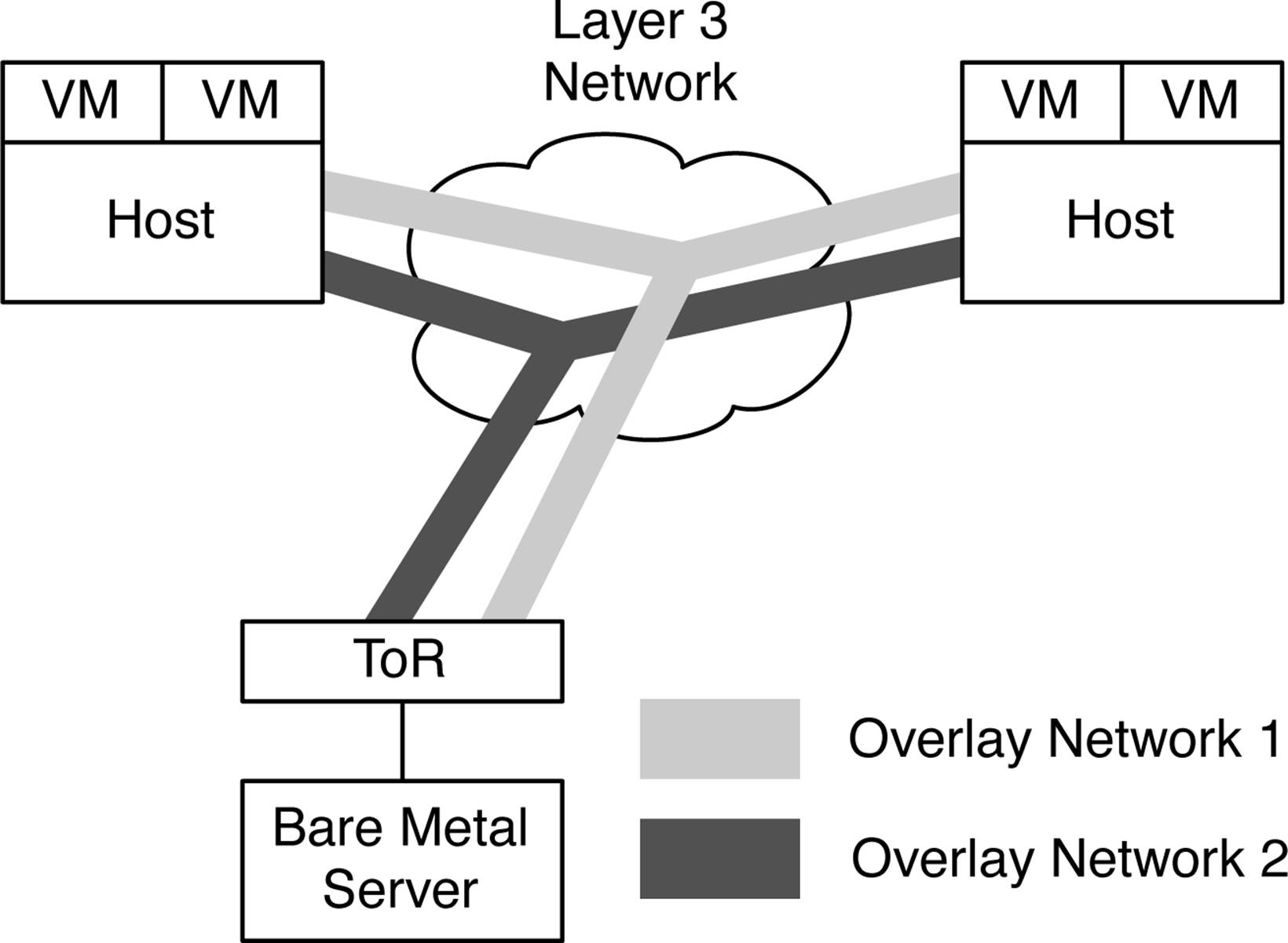
Figure 1-2. Overlay networking
The astute reader might have noticed in Figure 1-2 that in addition to supporting more than one overlay network, there are also virtualized and nonvirtualized workloads being connected by the overlay networks. In a production environment, there will always be a use case in which not all of the servers are virtualized but still need to communicate with virtual machines that are taking advantage of overlay networking. If the hypervisor is responsible for MAC address learning and termination of the overlay networks, this creates a challenge when a virtual machine needs to communicate with a bare-metal server. The solution is that the ToR switch can participate in the overlay network on behalf of nonvirtualized workloads, as is demonstrated in Figure 1-2. From the perspective of the bare-metal server, nothing changes; it sends to and receives traffic from the ToR, but the difference is that the ToR is configured to include the bare-metal server in the overlay network. With both the hypervisor and ToR handling all of the MAC address learning and overlay network termination, virtual machines and bare-metal servers are able to communicate and take full advantage of the overlay networks, such as those presented in Chapter 8.
The continued drive for high-density 10GbE access together with the evolutions of SDN and overlay networking are the key driving factors behind the introduction of the Juniper QFX5100 family in November 2013. Figure 1-3 illustrates that it is a set of data center Ethernet switches that can be used in the core, aggregation, and access tiers of the network. The Juniper QFX5100 was specifically designed to solve the high port density requirements of cloud computing and enable nonvirtualized workloads to participate in an overlay network architecture.
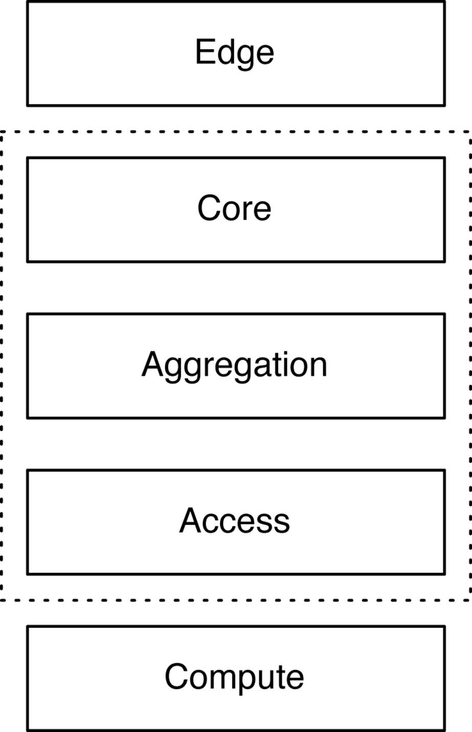
Figure 1-3. The data center roles and scope of the QFX5100 family
Having been specifically designed to solve cloud computing and SDN requirements, the Juniper QFX5100 family solves a wide variety of challenges and offers many unique benefits.
Transport
Dense 10GbE and 40GbE interfaces to build a deterministic spine-and-leaf topology with an option of 1:1, 3:1, or 6:1 over-subscription.
Interfaces
Each 10GbE interface is tri-speed and supports 100Mbps, 1GbE, or 10GbE. In addition, each interface can support either copper or fiber connectivity. Higher interface speeds such as 40GbE can be broken out into four 10bGE interfaces by using a breakout cable.
Overlay Networking
Each switch offers complete integration with Juniper Contrail and VMware NSX to support overlay networking. The Juniper QFX5100 family can be configured as an end point in an overlay network architecture to support bare-metal servers.
Latency
An intelligent algorithm is used for each ingress packet to determine which forwarding architecture—store-and-forward or cut-through—should be used to guarantee the least latency. On average the port-to-port latency is only 600 to 800 nanoseconds.
Flexible Deployment Options
The Juniper QFX5100 doesn’t force you to deploy a particular technology or proprietary protocol. It supports standalone, Virtual Chassis, QFabric node, Virtual Chassis Fabric, Multi-Chassis Link Aggregation (MC-LAG), or an IP Fabric architecture.
QFabric Node
The Juniper QFX5100 can be used as a node in the QFabric architecture. All of the benefits of the Juniper QFX5100 are available when used as a QFabric node: higher port density, overlay networking, and lower latency.
Virtualized Control Plane
The Juniper QFX5100 takes virtualization to heart. The control plane uses an Intel Sandy Bridge CPU. The host operating system is Linux running KVM and QEMU for virtualization. The network operating system (Junos) runs as a virtual machine and is able to take advantage of all of the benefits of virtualization such as In-Service Software Upgrade (ISSU).
Unified Forwarding Table
Whether you need to support more MAC addresses or IPv4 prefixes in an IP Fabric architecture, with the Juniper QFX5100, you can adjust the profile of the forwarding table. There are five preconfigured profiles that range between L2 heavy to L3 heavy.
Network Analytics
Some applications are sensitive to microbursts and latency. The Juniper QFX5100 allows you to get on-box reporting of queue depth, queue latency, and microburst detection to facilitate and speed up the troubleshooting process.
Lossless Ethernet
When converging storage and data, it’s critical that storage be handled in such a way that no traffic is dropped. The Juniper QFX5100 supports DCBX, ETS, and PFC to enable transit FCoE or lossless Ethernet for IP storage.
Virtual Chassis Fabric
Ethernet fabrics provide the benefit of a single point of management, lossless storage convergence, and full Layer 2 and Layer 3 services. The Juniper QFX5100 can form an Ethernet fabric called a Virtual Chassis Fabric (VCF). This is a spine-and-leaf topology that supports full Equal-Cost Multipath (ECMP) routing but with all of the benefits of an Ethernet fabric.
Inline Network Services
Traditionally, network services such as Generic Routing Encapsulation (GRE) and Network Address Translation (NAT) are handled by another device such as a router or firewall. The Juniper QFX5100 can perform both GRE and NAT in hardware without a performance loss. The Juniper QFX5100 also offers inline VXLAN termination for SDN and supports real-time networking analytics.
The Juniper QFX5100 family brings a lot of new features and differentiation to the table when it comes to solving data center challenges. Because of the wide variety of features and differentiation, you can integrate the Juniper QFX5100 into many different types of architectures.
High-Frequency Trading
Speed is king when it comes to trading stocks. With an average port-to-port latency of 550 nanoseconds, the Juniper QFX5100 fits well in a high-frequency trading architecture.
Private Cloud
Although the Juniper QFX5100 was specifically designed to solve the challenges of cloud computing and public clouds, you can take advantage of the same features to solve the needs of the private cloud. Enterprises, government agencies, and research institutes are building out their own private clouds, and the Juniper QFX5100 meets and exceeds all their requirements.
Campus
High port density and a single point of management make the Juniper QFX5100 a perfect fit in a campus architecture, specifically in the core and aggregation roles.
Enterprise
Offering the flexibility to be used in multiple deployment scenarios, the Juniper QFX5100 gives an enterprise the freedom to use the technology that best fits its needs. The Juniper QFX5100 can be used as a standalone device, a Virtual Chassis, a QFabric Node, a Virtual Chassis Fabric, a MC-LAG, or in a Clos architecture.
It’s a very exciting time in the networking industry as SDN, cloud computing, and data center technologies are continuing to push the envelope and bring new innovations and solutions to the field. The Juniper QFX5100 is embracing all of the change that’s happening and providing clear and distinctive solution differentiation. With its wide variety of features, the Juniper QFX5100 is able to quickly solve the challenges of cloud computing as well as other use cases such as high-frequency trading and campus.
Junos
Junos is a purpose-built networking operating system based on one of the most stable and secure operating systems in the world: FreeBSD. Junos is designed as a monolithic kernel architecture that places all of the operating system services in the kernel space. Major components of Junos are written as daemons that provide complete process and memory separation.
One of the benefits of monolithic kernel architecture is that kernel functions are executed in supervisor mode on the CPU, whereas the applications and daemons are executed in user space. A single failing daemon will not crash the operating system or impact other unrelated daemons. For example, if there were an issue with the Simple Network Management Protocol (SNMP) daemon and it crashed, it wouldn’t impact the routing daemon that handles Open Shortest Path First (OSPF) and Border Gateway Protocol (BGP).
One Junos
Creating a single network operating system that you can use across routers, switches, and firewalls simplifies network operations, administration, and maintenance. Network operators need only learn Junos once and become instantly effective across other Juniper products. An added benefit of a single Junos is that there’s no need to reinvent the wheel and have 10 different implementations of BGP or OSPF. Being able to write these core protocols once and then reuse them across all products provides a high level of stability because the code is very mature and field tested.
Software Releases
Every quarter for more than 15 years, there has been a consistent and predictable release of Junos. The development of the core operating system is a single-release train. This allows developers to create new features or fix bugs once and then share them across multiple platforms.
The release numbers are in a major and minor format. The major number is the version of Junos for a particular calendar year, and the minor release indicates in which trimester the software was released. There are a couple of different types of Junos that are released more frequently to resolve issues: maintenance and service releases. Maintenance releases are released about every six weeks to fix a collection of issues, and they are prefixed with “R.” For example, Junos 14.1R2 would be the second maintenance release for Junos 14.1. Service releases are released on demand to specifically fix a critical issue that has yet to be addressed by a maintenance release. These releases are prefixed with a “S.” An example would be Junos 14.1S2.
The general rule of thumb is that new features are added for every major and minor releases and bug fixes are added to service and maintenance releases. For example, Junos 14.1 to 14.2 would introduce new features, whereas Junos 14.1R1 to 14.1R2 would introduce bug fixes.
Most production networks prefer to use the last Junos release of the previous calendar year; these Junos releases are Extended End of Life (EEOL) releases that are supported for three years. The advantage is that the EEOL releases become more stable with time. Consider that 14.1 will stop providing bug fixes after 24 months, whereas 14.3 will continue to include bug fixes for 36 months.
Three-Release Cadence
In 2012, Junos created a new release model to move from four releases per year to three (Table 1-1 and Figure 1-4). This increased the frequency of maintenance releases to resolve more issues more often. The other benefit is that all Junos releases as of 2012 are supported for 24 months, whereas the last release of Junos for the calendar year will still be considered EEOL and have support for 36 months.
|
Release |
Target |
End of engineering |
End of life |
|
Junos 15.1 |
March |
24 months |
+ 6 months |
|
Junos 15.2 |
July |
24 months |
+ 6 months |
|
Junos 15.3 |
November |
36 months |
+ 6 months |
|
Table 1-1. Junos end-of-engineering and end-of-life schedule |
|||
By extending the engineering support and reducing the number of releases, network operators should be able to reduce the frequency of having to upgrade to a new release of code.
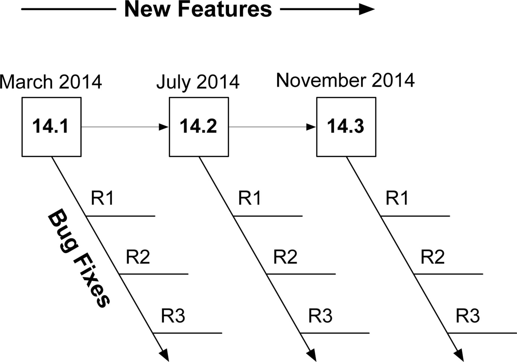
Figure 1-4. Junos three-release cadence
With the new Junos three-release cadence, network operators can be more confident using any version of Junos without feeling pressured to only use the EEOL release.
Software Architecture
Junos was designed from the beginning to support a separation of control and forwarding plane. This is true of the Juniper QFX5100 series for which all of the control plane functions are performed by the routing engine, whereas all of the forwarding is performed by the Packet Forwarding Engine (PFE) (Figure 1-5). Providing this level of separation ensures that one plane doesn’t impact the other. For example, the forwarding plane could be forwarding traffic at line rate and performing many different services while the routing engine sits idle and unaffected.
Control plane functions come in many shapes and sizes. There’s a common misconception that the control plane only handles routing protocol updates. In fact, there are many more control plane functions. Some examples include:
§ Updating the routing table
§ Answering SNMP queries
§ Processing SSH or HTTP traffic to administer the switch
§ Changing fan speed
§ Controlling the craft interface
§ Providing a Junos micro kernel to the PFEs
§ Updating the forwarding table on the PFEs
Figure 1-5. Junos software architecture
At a high level, the control plane is implemented entirely within the routing engine, whereas the forwarding plane is implemented within each PFE using a small, purpose-built kernel that contains only the required functions to forward traffic.
The benefit of control and forwarding separation is that any traffic that is being forwarded through the switch will always be processed at line rate on the PFEs and switch fabric; for example, if a switch were processing traffic between web servers and the Internet, all of the processing would be performed by the forwarding plane.
Daemons
The Junos kernel has five major daemons. Each of these daemons play a critical role within the Juniper QFX5100 and work together via Interprocess Communication (IPC) and routing sockets to communicate with the Junos kernel and other daemons. These daemons, which take center stage and are required for the operation of Junos, are listed here:
§ Management daemon (mgd)
§ Routing protocol daemon (rpd)
§ Device control daemon (dcd)
§ Chassis daemon (chassisd)
§ Analytics daemon (analyticsd)
There are many more daemons for tasks such as NTP, VRRP, DHCP, and other technologies, but they play a smaller and more specific role in the software architecture. The sections that follow provide descriptions of each of the five major daemons.
Management daemon
The Junos User Interface (UI) keeps everything in a centralized database. This makes it possible for Junos to handle data in interesting ways and opens the door to advanced features such as configuration rollback, apply groups, and activating and deactivating entire portions of the configuration.
The UI has four major components: the configuration database, database schema, management daemon, and the command-line interface (CLI).
The management daemon is the glue that holds the entire Junos UI together. At a high level, it provides a mechanism to process information for both network operators and daemons.
The interactive component of the management daemon is the Junos CLI. This is a terminal-based application that provides the network operator with an interface into Junos. The other side of the management daemon is the XML remote procedure call (RPC) interface. This provides an API through Junoscript and Netconf to accommodate the development of automation applications.
Following are the cli responsibilities:
§ Command-line editing
§ Terminal emulation
§ Terminal paging
§ Displaying command and variable completions
§ Monitoring log files and interfaces
§ Executing child processes such as ping, traceroute, and ssh
The management daemon responsibilities include the following:
§ Passing commands from the cli to the appropriate daemon
§ Finding command and variable completions
§ Parsing commands
It’s interesting to note that the majority of the Junos operational commands use XML to pass data. To see an example of this, simply add the pipe command display xml to any command. Let’s take a look at a simple command such as show isis adjacency:
{master}
dhanks@R1-RE0> show isis adjacency
Interface System L State Hold (secs) SNPA
ae0.1 R2-RE0 2 Up 23
So far, everything looks normal. Let’s add the display xml to take a closer look:
{master}dhanks@R1-RE0> show isis adjacency | display xml
<rpc-reply xmlns:junos="http://xml.juniper.net/junos/11.4R1/junos">
<isis-adjacency-information xmlns="http://xml.juniper.net/junos/11.4R1/junos-
routing" junos:style="brief">
<isis-adjacency>
<interface-name>ae0.1</interface-name>
<system-name>R2-RE0</system-name>
<level>2</level>
<adjacency-state>Up</adjacency-state>
<holdtime>22</holdtime>
</isis-adjacency>
</isis-adjacency-information>
<cli>
<banner>{master}</banner>
</cli>
</rpc-reply>
As you can see, the data is formatted in XML and received from the management daemon via RPC.
Routing protocol daemon
The routing protocol daemon handles all of the routing protocols configured within Junos. At a high level, its responsibilities are receiving routing advertisements and updates, maintaining the routing table, and installing active routes into the forwarding table. To maintain process separation, each routing protocol configured on the system runs as a separate task within the routing protocol daemon. Its other responsibility is to exchange information with the Junos kernel to receive interface modifications, send route information, and send interface changes.
Let’s take a peek into the routing protocol daemon and see what’s going on. The hidden command set task accounting toggles CPU accounting on and off. Use show task accounting to see the results:
{master}
dhanks@R1-RE0> set task accounting on
Task accounting enabled.
Now, we’re good to go. Junos is currently profiling daemons and tasks to get a better idea of what’s using the CPU. Let’s wait a few minutes for it to collect some data.
OK, let’s check it out:
{master}
dhanks@R1-RE0> show task accounting
Task accounting is enabled.
Task Started User Time System Time Longest Run
Scheduler 265 0.003 0.000 0.000
Memory 2 0.000 0.000 0.000
hakr 1 0.000 0 0.000
ES-IS I/O./var/run/ppmd_c 6 0.000 0 0.000
IS-IS I/O./var/run/ppmd_c 46 0.000 0.000 0.000
PIM I/O./var/run/ppmd_con 9 0.000 0.000 0.000
IS-IS 90 0.001 0.000 0.000
BFD I/O./var/run/bfdd_con 9 0.000 0 0.000
Mirror Task.128.0.0.6+598 33 0.000 0.000 0.000
KRT 25 0.000 0.000 0.000
Redirect 1 0.000 0.000 0.000
MGMT_Listen./var/run/rpd_ 7 0.000 0.000 0.000
SNMP Subagent./var/run/sn 15 0.000 0.000 0.000
There’s not too much going on here, but you get the idea. Currently, running daemons and tasks within the routing protocol daemon are present and accounted for.
WARNING
The set task accounting command is hidden for a reason. It’s possible to put additional load on the Junos kernel while accounting is turned on. It isn’t recommended to run this command on a production network unless instructed by the Juniper Technical Assistance Center (JTAC). After your debugging is finished, don’t forget to turn it back off by using set task accounting off.
{master}
dhanks@R1-RE0> set task accounting off
Task accounting disabled.
Device control daemon
The device control daemon is responsible for setting up interfaces based on the current configuration and available hardware. One feature of Junos is the ability to configure nonexistent hardware. This is based on the underlying assumption that the hardware can be added at a later date and “just work.” For example, you can configure set interfaces ge-1/0/0.0 family inet address 192.168.1.1/24 and commit. Assuming there’s no hardware in FPC1, this configuration will not do anything. However, as soon as hardware is installed into FPC1, the first port will be configured immediately with the address 192.168.1.1/24.
Chassis daemon (and friends)
The chassis daemon supports all chassis, alarm, and environmental processes. At a high level, this includes monitoring the health of hardware, managing a real-time database of hardware inventory, and coordinating with the alarm daemon and the craft daemon to manage alarms and LEDs.
It should all seem self-explanatory except for the craft daemon, the craft interface that is the front panel of the device. Let’s take a closer look at the Juniper QFX5100 craft interface in Figure 1-6.
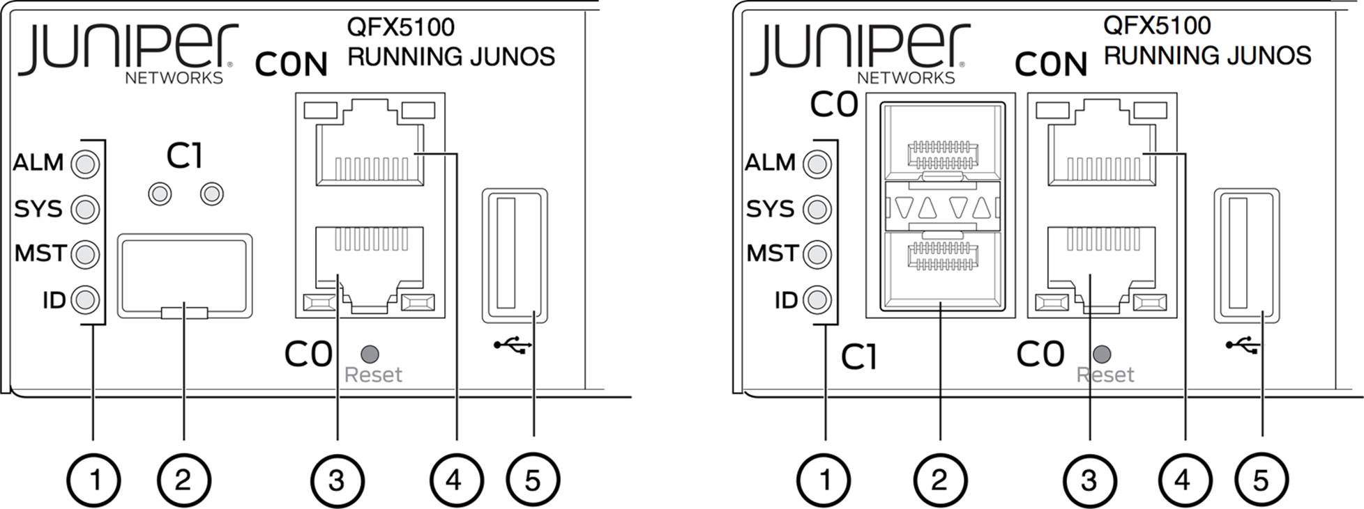
Figure 1-6. The Juniper QFX5100 craft interface
It’s simply a collection of buttons and LED lights to display the current status of the hardware and alarms. Let’s inspect the LEDs shown in Figure 1-6 a bit closer.
1. Status LEDs.
2. em1-SFP management Ethernet port (C1) cage. It can support either 1GbE copper SFP or fiber SFP.
3. em0-RJ-45 (1000BASE-T) management Ethernet port (C0).
4. RJ-45/RS-232 console port (CON).
5. USB port.
This information can also be obtained via the command line as well with the command show chassis led, as illustrated here:
{master:0}
dhanks@QFX5100> show chassis led
LED status for: FPC 0
-----------------------------------
LEDs status:
Alarm LED : Yellow
System LED : Green
Master LED : Green
Beacon LED : Off
QIC 1 STATUS LED : Green
QIC 2 STATUS LED : Green
Interface STATUS LED LINK/ACTIVITY LED
---------------------------------------------------------
et-0/0/0 N/A Green
et-0/0/1 N/A Green
et-0/0/2 N/A Green
et-0/0/3 N/A Off
et-0/0/4 N/A Green
et-0/0/5 N/A Green
et-0/0/8 N/A Off
et-0/0/9 N/A Off
et-0/0/11 N/A Off
One final responsibility of the chassis daemon is monitoring the power and cooling environmentals. It constantly monitors the voltages of all components within the chassis and will send alerts if any of those voltages cross specified thresholds. The same is true for the cooling. The chassis daemon constantly monitors the temperature on all of the components and chips as well as fan speeds. If anything is out of the ordinary, it will create alerts. Under extreme temperature conditions, the chassis daemon can also shut down components to avoid damage.
Analytics daemon
When troubleshooting a network, it’s common to ask yourself the following questions:
§ Why isn’t the application behaving as expected?
§ Why is the network slow?
§ Am I meeting my service level agreements?
To help answer these questions, the Juniper QFX5100 brings a new daemon into the mix: the analytics daemon. The analytics daemon provides detailed data and reporting on the network’s behavior and performance. The data collected can be broken down into two types:
Queue Statistics
Each port on the switch has the ability to queue data before it is transmitted. The ability to queue data not only ensures the delivery of traffic, but it also impacts the end-to-end latency. The analytics daemon reports data on the queue latency and queue depth at a configured time interval on a per-interface basis.
Traffic Statistics
Being able to measure the packets per second (pps), packets dropped, port utilization, and number of errors on a per-interface basis gives you the ability to quickly graph the network.
You can access the data collected by the analytics daemon in several different ways. You can store it on the local device or stream it to a remote server in several different formats.
Traffic must be collected from two locations within the switch in order for the data to be accurate. The first location to collect traffic is inside the analytics module in the PFE; this permits the most accurate statistics possible without impacting the switch’s performance. The second location to collect traffic is from the routing engine. The PFE sends data to the routing engine if that data exceeds certain thresholds. The analytics daemon will then aggregate the data. The precise statistics directly from the PFE and the aggregated data from the routing engine is combined to give you a complete, end-to-end view of the queue and traffic statistics of the network.
Network analytics is covered in more depth in Chapter 9.
Routing Sockets
Routing sockets are a UNIX mechanism for controlling the routing table. The Junos kernel takes this same mechanism and extends it to include additional information to support additional attributes to create a carrier-class network operating system.
At a high level, there are two actors that use routing sockets: the state producer and the state consumer. The routing protocol daemon is responsible for processing routing updates and thus is the state producer. Other daemons are considered a state consumer because they process information received from the routing sockets, as demonstrated in Figure 1-7.
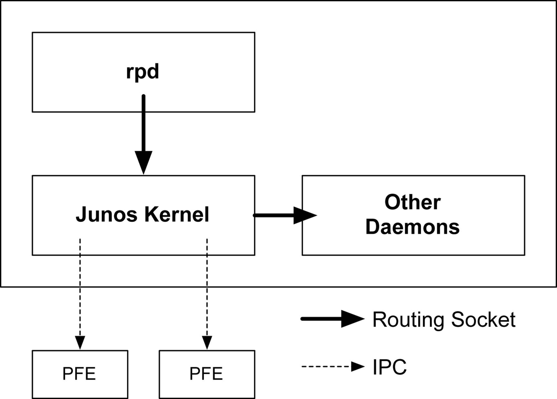
Figure 1-7. Routing socket architecture
Let’s take a peek into the routing sockets and see what happens when we configure ge-1/0/0.0 with an IP address of 192.168.1.1/24. Using the rtsockmon command from the shell allows us to see the commands being pushed to the kernel from the Junos daemons.
{master}
dhanks@R1-RE0> start shell
dhanks@R1-RE0% rtsockmon -st
sender flag type op
[16:37:52] dcd P iflogical add ge-1/0/0.0 flags=0x8000
[16:37:52] dcd P ifdev change ge-1/0/0 mtu=1514 dflags=0x3
[16:37:52] dcd P iffamily add inet mtu=1500 flags=0x8000000200000000
[16:37:52] dcd P nexthop add inet 192.168.1.255 nh=bcst
[16:37:52] dcd P nexthop add inet 192.168.1.0 nh=recv
[16:37:52] dcd P route add inet 192.168.1.255
[16:37:52] dcd P route add inet 192.168.1.0
[16:37:52] dcd P route add inet 192.168.1.1
[16:37:52] dcd P nexthop add inet 192.168.1.1 nh=locl
[16:37:52] dcd P ifaddr add inet local=192.168.1.1
[16:37:52] dcd P route add inet 192.168.1.1 tid=0
[16:37:52] dcd P nexthop add inet nh=rslv flags=0x0
[16:37:52] dcd P route add inet 192.168.1.0 tid=0
[16:37:52] dcd P nexthop change inet nh=rslv
[16:37:52] dcd P ifaddr add inet local=192.168.1.1 dest=192.168.1.0
[16:37:52] rpd P ifdest change ge-1/0/0.0, af 2, up, pfx 192.168.1.0/24
NOTE
For the preceding example, I configured the interface ge-1/0/0 in a different terminal window and committed the change while the rtstockmon command was running.
The command rtsockmon is a Junos shell command that gives the user visibility into the messages being passed by the routing socket. The routing sockets are broken into four major components: sender, type, operation, and arguments. The sender field is used to identify which daemon is writing into the routing socket. The type identifies which attribute is being modified. The operation is showing what is actually being performed. There are three basic operations: add, change, and delete. The last field is the arguments passed to the Junos kernel. These are sets of key/value pairs that are being changed.
In the previous example, you can see how dcd interacts with the routing socket to configure ge-1/0/0.0 and assign an IPv4 address.
§ dcd creates a new logical interface (IFL).
§ dcd changes the interface device (IFD) to set the proper Maximum Transmission Unit (MTU).
§ dcd adds a new interface family (IFF) to support IPv4.
§ dcd sets the nexthop, broadcast, and other attributes that are needed for the Routing Information Base (RIB) and Forwarding Information Base (FIB).
§ dcd adds the interface address (IFA) of 192.168.1.1.
§ rpd finally adds a route for 192.168.1.1 and brings it up.
WARNING
The rtsockmon command is used only to demonstrate the functionality of routing sockets and how daemons such as dcd and rpd use routing sockets to communicate routing changes to the Junos kernel.
QFX5100 Platforms
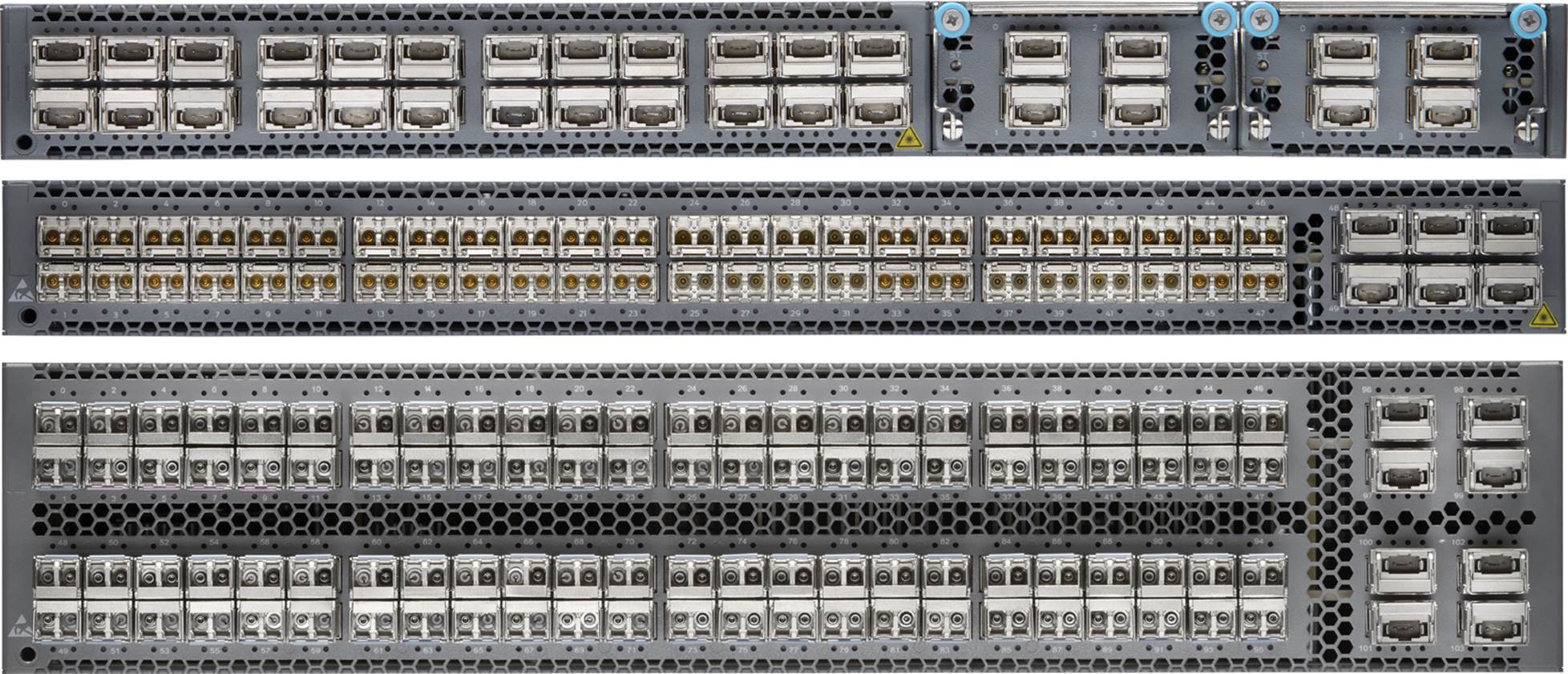
Figure 1-8. The Juniper QFX5100 series
The Juniper QFX5100 series (Figure 1-8) is available in four models. Each has varying numbers of ports and modules, but they share all of the same architecture and benefits. Depending on the number of ports, modules, and use case, a particular model can fit into multiple roles of a data center or campus architecture. In fact, it’s common to see the same model of switch in multiple roles in an architecture. For example, if you require 40GbE access, you can use the Juniper QFX5100-24Q in all three roles: core, aggregation, and access. Let’s take a look at each model and see how they compare to one another:
QFX5100-24Q
First is the Juniper QFX5100-24Q; this model has 24 40GbE interfaces and two modules that allow for expansion. In a spine-and-leaf architecture, this model is most commonly deployed as a spine fulfilling the core and aggregation roles.
QFX5100-48S
Next is the Juniper QFX5100-48S; this model has 48 10GbE interfaces as well as 6 40GbE interfaces. There are no modules, but there is enough bandwidth to provide 2:1 over-subscription. There is 480 Gbps of downstream bandwidth from the 48 10GbE interfaces and 240 Gbps of upstream bandwidth from the 6 40bGE interfaces. In a spine-and-leaf architecture, this model is most commonly deployed as a leaf fulfilling the access role.
QFX5100-96S
When you need to go big, the Juniper QFX5100-96S offers 96 10GbE and 8 40GbE interfaces to maintain an optimal 3:1 over-subscription. In a spine-and-lead architecture, this model is most commonly deployed as a leaf.
Now that you have an idea of the different models that are available in the Juniper QFX5100 series, let’s compare and contrast them in the matrix shown in Table 1-2 so that you can easily see the differences.
|
Attribute |
QFX5100 24Q |
QFX5100 48S |
QFX5100 48T |
QFX5100 96S |
|
10GbE ports |
0 |
48 |
48 |
96 |
|
40GbE ports |
24 |
6 |
6 |
8 |
|
Modules |
2 |
0 |
0 |
0 |
|
Rack units |
1 |
1 |
1 |
2 |
|
Table 1-2. QFX5100 series model comparison |
||||
Depending on how many modules and which specific module is used, the port count can change for the models that have expansion ports. For example, the Juniper QFX5100-24Q has 24 40GbE built-in interfaces, but using two modules can increase the total count to 32 40GbE interfaces, with the assumption that each module has 4 40GbE interfaces. Each model has been specifically designed to operate in a particular role in a data center or campus architecture but offer enough flexibility that a single model can operate in multiple roles.
QFX5100 Modules
The modules make it possible for you to customize the Juniper QFX5100 series to suit the needs of the data center or campus. Depending on the port count and speed of the module, each model can easily be moved between roles in a data center architecture. Let’s take a look at the modules available as of this writing:
4 40GbE QIC
Using this module, you can add an additional 160 Gbps of bandwidth via 4 40GbE interfaces. You can use the interfaces as-is or they can be broken out into 16 10GbE interfaces with a breakout cable.
8 10GbE QIC
This module adds an additional 80 Gbps of bandwidth via 8 10GbE interfaces. It’s a great module to use when you need to add a couple more servers into a rack, assuming the built-in switch interfaces are in use. The eight 10GbE QIC also supports data plane encryption on all eight ports with Media Access Control Security (MACsec).
The QFX Interface Card (QIC) allows you to selectively increase the capacity of the Juniper QFX5100 platforms. Generally, you use the 4 40GbE module for adding additional upstream bandwidth on a ToR or simply filling out the 40GbE interfaces in a spine such as the Juniper QFX5100-24Q. You typically use the 8 10GbE module to add additional downstream bandwidth for connecting compute resources.
QFX5100-24Q
The Juniper QFX5100-24Q (see Figure 1-9) is the workhorse of the Juniper QFX5100 family of switches. In a data center architecture, it can fulfill the roles of the core, aggregation, and access. In a spine-and-leaf topology, it’s most commonly used as the spine that interconnects all of the leaves, as shown in Figure 1-10.
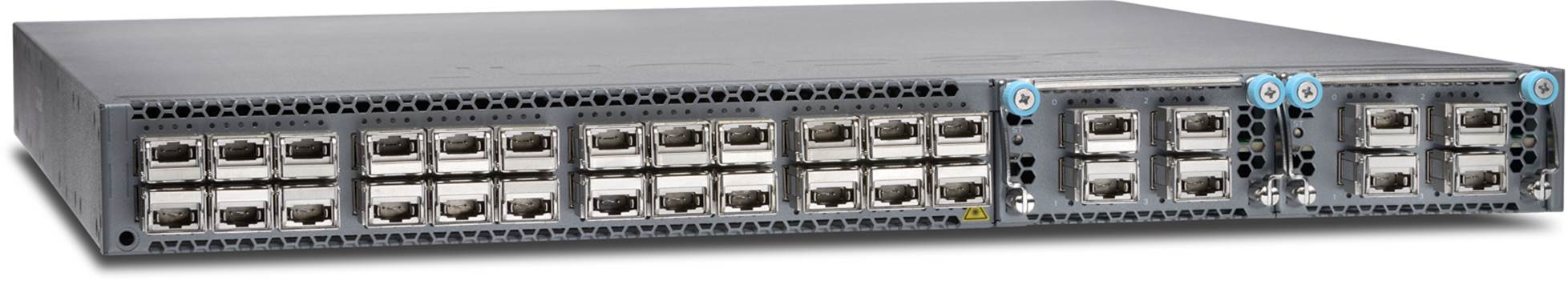
Figure 1-9. The Juniper QFX5100-24Q switch
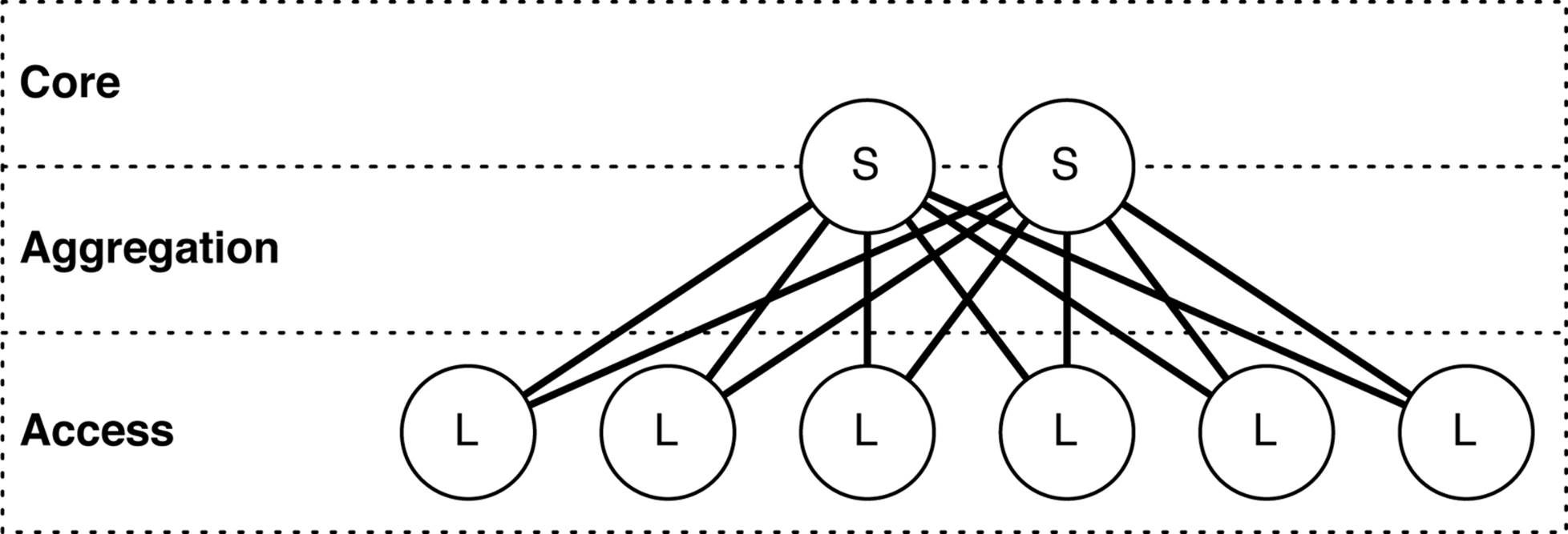
Figure 1-10. Spine-and-leaf topology and data center roles
Roles
An interesting aspect of the Juniper QFX5100-24Q is that it’s able to collapse both the core and aggregation roles in a data center architecture. In Figure 1-10, the Juniper QFX5100-24Q is represented by the spine (denoted with an “S”), which is split between the core and aggregation roles. The reason the Juniper QFX5100-24Q is able to collapse the core and aggregation roles is because it offers both high-speed and high-density ports in a single switch.
Module options
The most typical configuration of the Juniper QFX5100-24Q uses a pair of four 40GbE modules, as depicted in Figure 1-11. The combination of built-in ports and modules brings the total interface count to 32 40GbE.
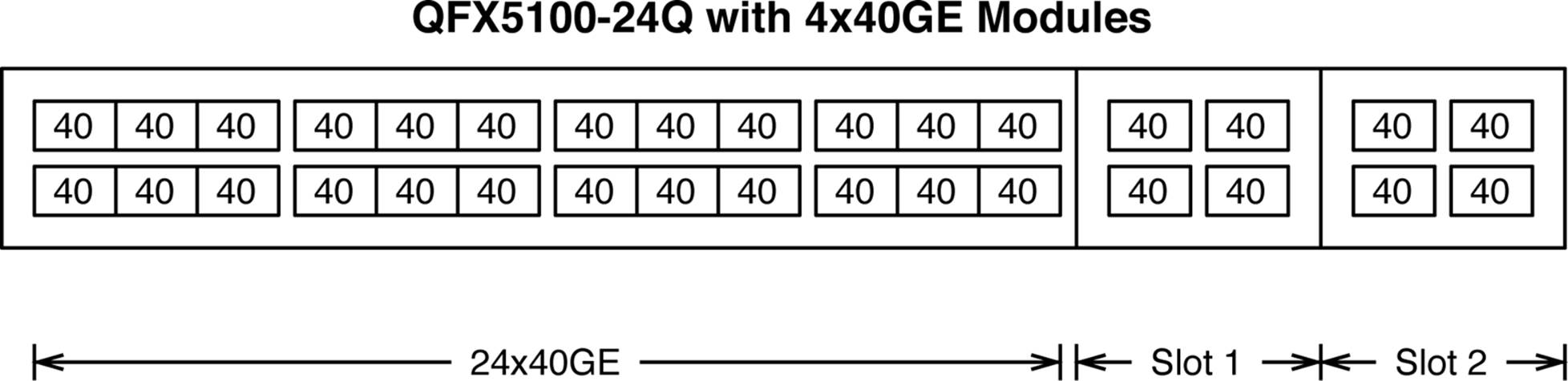
Figure 1-11. The Juniper QFX5100-24Q interface and slot layout using four 40GbE modules
A second configuration using a pair of eight 10GbE QICs can change the Juniper QFX5100-24Q to support 24 40GbE and 16 10GbE interfaces, as illustrated in Figure 1-12.
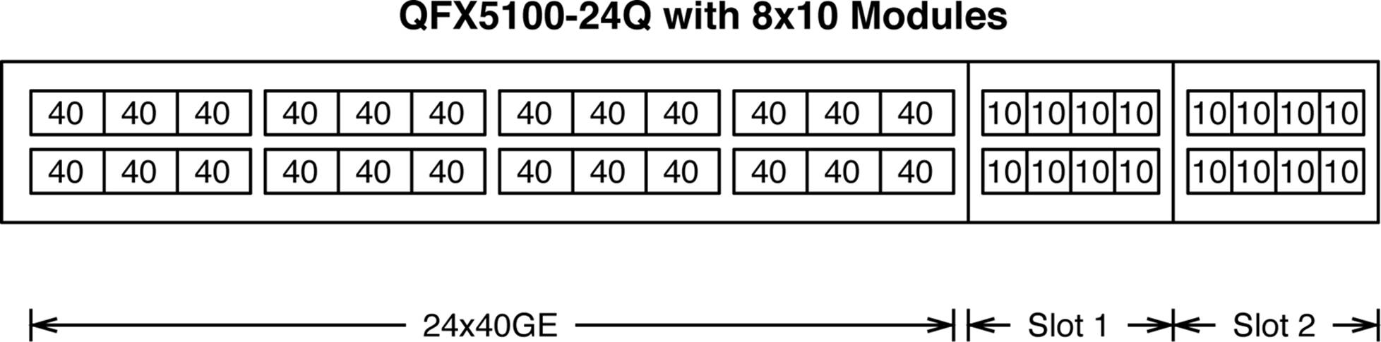
Figure 1-12. The Juniper QFX5100-24Q interface and slot layout using 8×10GE modules
Although the Juniper QFX5100-24Q using the four 40GbE QICs is well suited in the core and aggregation of a spine-and-leaf topology, the eight 10GbE QIC transforms the switch so that it’s more suitable as a leaf in the access layer. With a combination of both 10GbE and 40GbE, the Juniper QFX5100-24Q is now able to support a combination of compute resources. In addition, you can still use the switch in the core and aggregation layer in the spine of the topology, but allow other components such as an edge router, firewall, or load balancer to peer directly with the spine, as shown in Figure 1-13.
Let’s take a look at Figure 1-13 in more detail to fully understand how you can deploy the Juniper QFX5100-24Q in different roles of an architecture. The spines S1 and S2 are a pair of QFX5100-24Q using the eight 10GbE QICs, which allow the edge routers E1 and E2 to have 10GbE connectivity directly with the spine switches S1 and S2 in the core and aggregation roles. When the Juniper QFX5100-24Q uses the eight 10GbE QICs, it has the flexibility to offer both 10GbE and 40GbE interfaces.
Figure 1-13. The QFX5100-24Q in multiple roles in a spine-and-leaf architecture
In the access role, there are two QFX5100-24Q switches, illustrated as L1 and L2. These switches are providing 40GbE access interfaces to Host 1. The other two access switches, L3 and L4, are a pair of QFX5100-48S switches and provide 10GbE access to Host 2.
Physical attributes
The Juniper QFX5100-24Q is a very flexible switch that you can deploy in a variety of roles in a network. Table 1-3 takes a closer look at the switch’s physical attributes.
|
Physical attributes |
Value |
|
Rack units |
1 |
|
Built-in interfaces |
24 40GbE |
|
Total 10GbE interfaces |
104 using breakout cables |
|
Total 40GbE interfaces |
32, using two four 40GbE modules |
|
Modules |
2 |
|
Airflow |
Airflow in (AFI) or airflow out (AFO) |
|
Power |
150 |
|
Cooling |
5 fans with N + 1 redundancy |
|
PFEs |
1 |
|
Latency |
~500 nanoseconds |
|
Buffer size |
12 MB |
|
Table 1-3. Physical attributes of the QFX5100-24Q |
|
The Juniper QFX5100-24Q packs quite a punch in a small 1RU form factor. As indicated by the model number, the Juniper QFX5100-24Q has 24 40GbE built-in interfaces, but it can support up to 104 10GbE interfaces by using a breakout cable. Although the math says that with 32 40GbE interfaces you should be able to get 128 10GbE interfaces, the PFE has a limitation of 104 total interfaces at any given time. There are two available QIC modules to further expand the switch to support additional 10GbE or 40GbE interfaces.
Cooling is carried out by a set of five fans in a “4 + 1” redundant configuration. You can configure the Juniper QFX5100-24Q to cool front-to-back (AFO) or back-to-front (AFI).
WARNING
Although the Juniper QFX5100-24Q fans support both AFO and AFI airflow, it’s important to match the same airflow with the power supplies. This way, both the fans and power supplies have the same airflow, and the switch is cooled properly. Mismatching the airflow could result in the switch overheating.
The switch is powered by two power supplies. Each power supply can support either AFO or AFI airflow; it’s critical that the airflow of the power supply match the airflow of the fans, as shown in Figure 1-14.
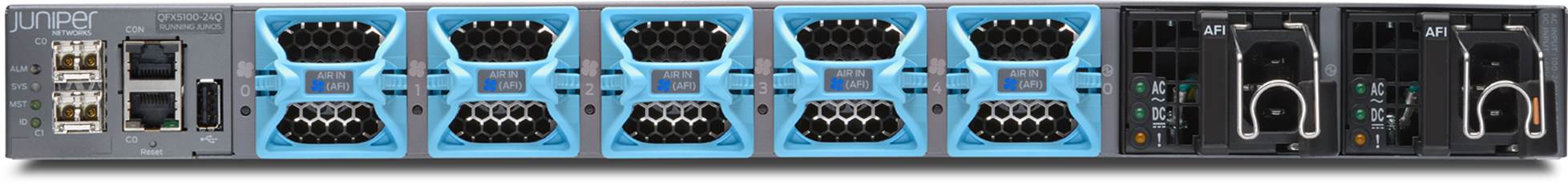
Figure 1-14. The rear of the Juniper QFX5100-24Q, illustrating the AFI airflow on the fans and power supplies
A really great feature of the Juniper QFX5100 is the colored plastic on the rear of the switch. The handles to remove the fans and power supplies are color-coded to indicate the direction of airflow.
Blue (AFI)
Blue represents cool air coming into the rear of the switch, which creates a back-to-front airflow through the chassis.
Orange (AFO)
Orange represents hot air exiting the rear of the switch, which creates a front-to-back airflow through the chassis.
Previously, the AFI and AFO notations were a bit confusing, but with the new color-coding, it’s no longer an issue. Being able to quickly identify the type of airflow prevents installation errors and gives you peace of mind.
The rear of the Juniper QFX5100-24Q has three main components, as illustrated in Figure 1-15. These components are management, cooling, and power. The management section (shown on the left in Figure 1-15) has a combination of SFP, 1000BASE-T, RS232, and USB connectivity.
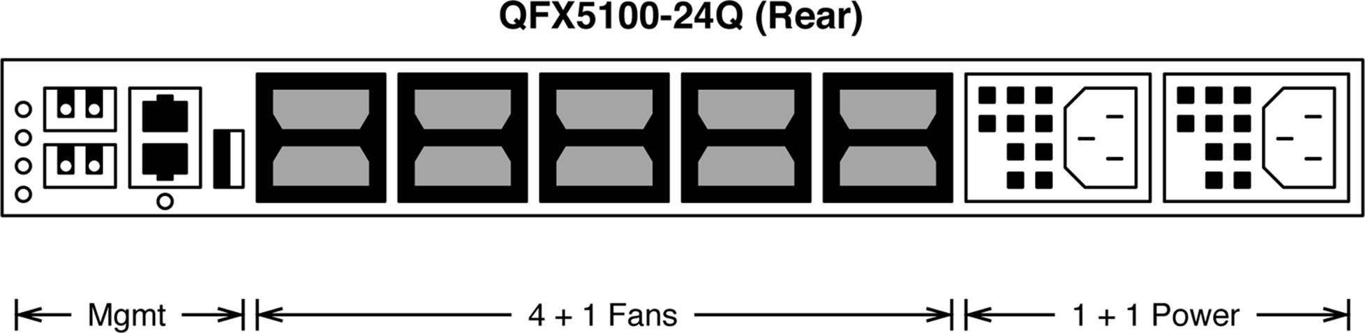
Figure 1-15. View of the rear of the Juniper QFX5100-24Q
There are a total of five fans on the Juniper QFX5100-24, and each one is a field replaceable unit (FRU). The fans are designed in a 4 + 1 redundancy model so that any one of the fans can fail, but the system will continue to operate normally. There is a total of two power supplies operating in a 1 + 1 redundancy configuration. A power supply can experience a failure, and the other power supply has enough output to allow the switch to operate normally.
Management
The management interfaces on the Juniper QFX5100 are very similar to the existing QFX3500 and QFX3600 family. There are six status LEDs, three management ports, an RS-232 port, and a USB port, as illustrated in Figure 1-16.
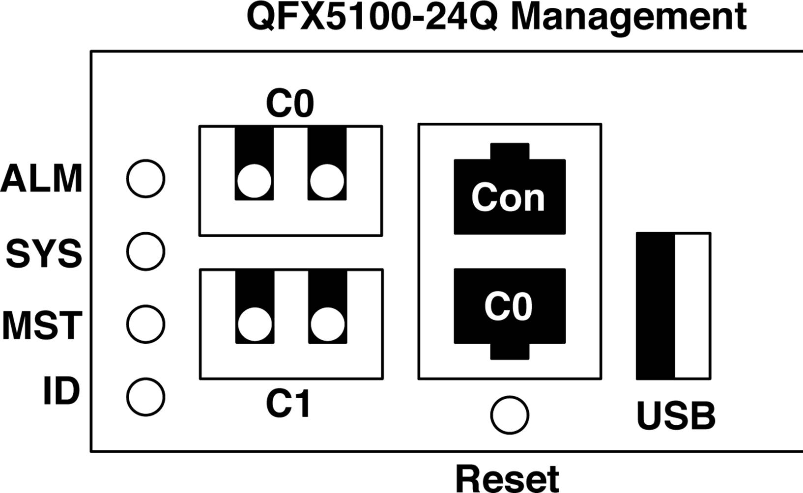
Figure 1-16. The QFX5100-24Q management console
Let’s walk through the status LEDs, one by one:
ALM (Alarm)
The ALM LED can be either red or amber depending on the severity of the alarm. If the alarm is red, this is an indication that one or more hardware components have failed or have exceeded temperature thresholds. An amber alarm indicates a noncritical issue, but if left unchecked, it could result in a service interruption.
SYS (System)
This LED is always green but has three illumination states: steady, blinking, or off. If the SYS LED is steady and always on, this means that Junos has been properly loaded onto the switch. If the SYS LED is blinking, this means that the switch is still booting. Finally, if the SYS LED is off, it means that the switch is powered off or has been halted.
MST (Master)
Similar to SYS, the MST LED is always green and has the same three states: steady, blinking, or off. If the MST LED is steady, the switch is currently the master routing engine of a Virtual Chassis. If the MST LED is blinking, the switch is the backup routing engine in a Virtual Chassis. If the MST LED is off, the switch is either a line card in Virtual Chassis or it’s operating as a standalone switch.
ID (Identification)
This is a new LED, first appearing on the Juniper QFX5100 family. It is here to help remote hands and the installation of the switch; you can use it to help identify a particular switch with a visual indicator. The ID LED is always blue and has two states: on or off. When the ID LED is on, the beacon feature has been enabled through the command line of the switch. If the ID LED is off, this is the default state and indicates that the beacon feature is currently disabled on the switch.
There are three management ports in total, but you can use only two at any given time; these are referred to as C0 and C1. The supported combinations are presented in Table 1-4:
|
C0 |
C1 |
Transceiver |
|
SFP |
SFP |
1G-SR, 1G-SR |
|
SFP |
SFP |
1G-SR, 1G-T |
|
SFP |
SFP |
1G-T, 1G-SR |
|
SFP |
SFP |
1G-T, 1G-T |
|
RJ-45 |
SFP |
N/A, 1G-SR |
|
RJ-45 |
SFP |
N/A, 1G-T |
|
Table 1-4. Valid QFX5100 management port combinations |
||
Basically, the two C0 management ports are interchangeable, but you can use only one at any given time. The C0 and C1 SFP management port can support either 1G-SR or 1G-T transceivers.
The two management ports C0 and C1 are used for out-of-band management. Typically, only a single management port will be used, but for the scenario in which the Juniper QFX5100 is being used as a QFabric Node, both ports are required, as depicted in Figure 1-17.
In a QFabric architecture, each node and interconnect requires two out-of-band management connections to ensure redundancy. The out-of-band management connections are used purely for the control plane, whereas the 40GbE interfaces are used for the data plane, as illustrated in Figure 1-17. Having both a SFP and copper management port gives you more installation flexibility in the data center. If you prefer fiber, you can easily use just the C1 interface and leave C0 unused. If the switch is being used as a QFabric Node and you require both management ports but only want to use copper, the SFP supports using a 1GE-T transceiver.
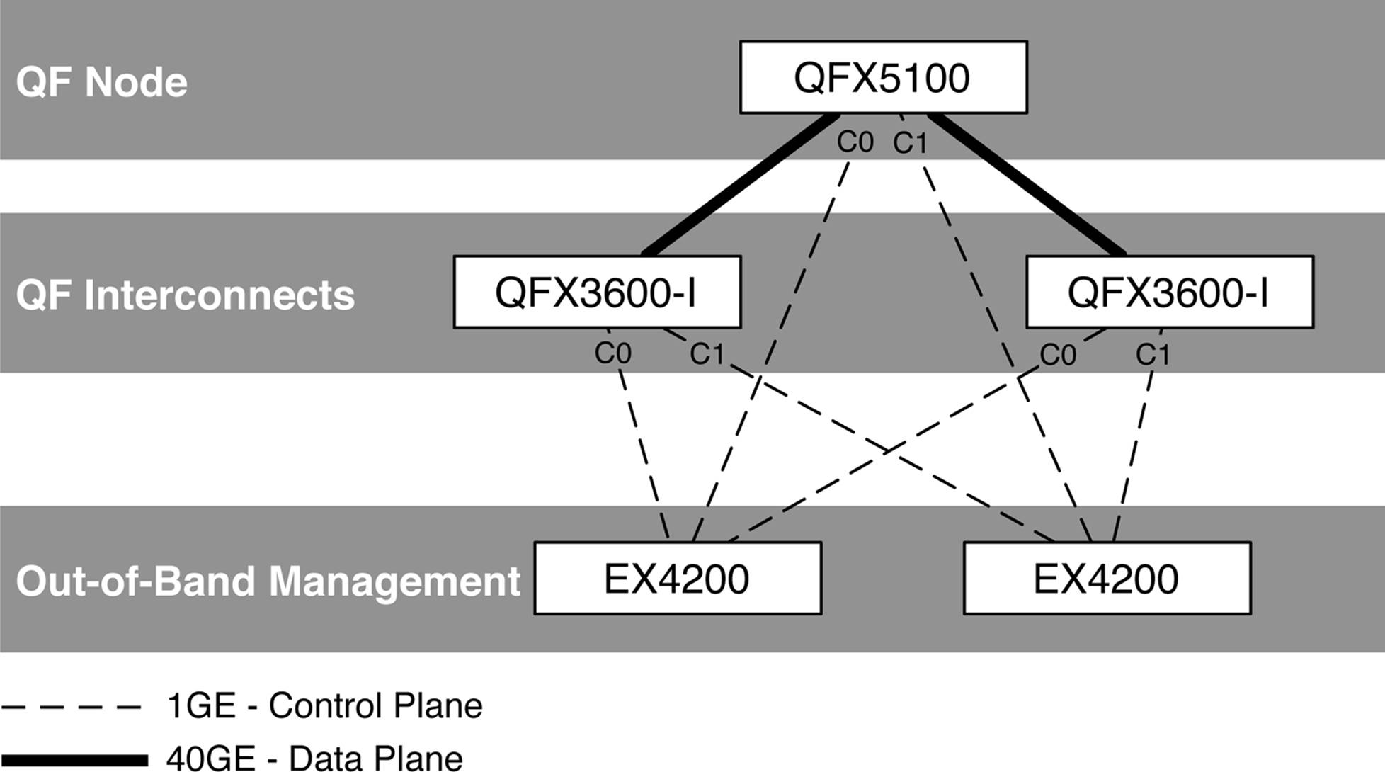
Figure 1-17. The C0 and C1 management ports in a QFabric Node topology
The RS-232 console port is a standard RJ-45 interface. This serial port is used to communicate directly with the routing engine of the switch. For situations in which the switch becomes unreachable by IP, the serial RS-232 is always a nice backup to have.
The USB port is a standard USB 2.0 interface and can be used with any modern thumb drive storage media. Again, for the scenario in which IP connectivity isn’t available, you can use the USB port to load software directly onto the switch. The USB port combined with the RS-232 serial console give you full control over the switch.
QFX5100-48S
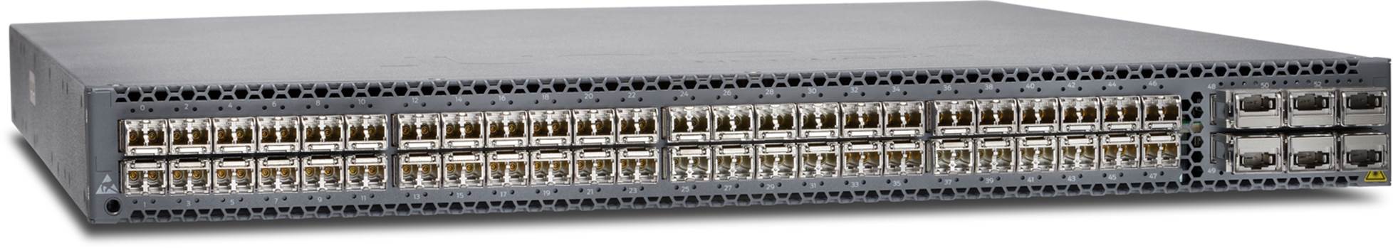
Figure 1-18. The Juniper QFX5100-48S switch
The Juniper QFX5100-48S (Figure 1-18) is another workhorse in the Juniper QFX5100 family of switches. In a data center architecture, it has been designed to fulfill the role of the access tier. In a spine-and-leaf topology, it’s most commonly used as the leaf that offers connectivity to end hosts, as shown in Figure 1-19.
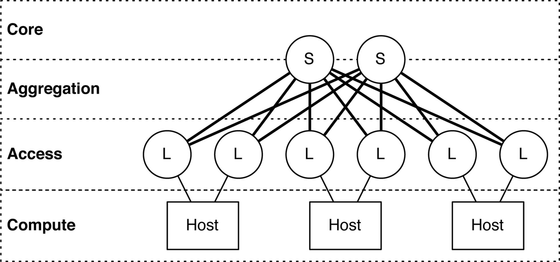
Figure 1-19. Spine-and-leaf topology, with the Juniper QFX5100-48S as a leaf
Roles
The primary role for the Juniper QFX5100-48S is to operate in the access tier of a data center architecture, due to the high density of 10GbE ports. In Figure 1-19, the “L” denotes the Juniper QFX5100-48S in a spine-and-leaf topology; “S” indicates the Juniper QFX5100-24Q being used in the spine. The Juniper QFX5100-24Q and QFX5100-48S were specifically designed to work together to build a spine-and-leaf topology and offer an option of 2:1 or 3:1 over-subscription.
The front of the Juniper QFX5100-48S offers two sets of built-in interfaces: 48 10GbE interfaces and 6 40GbE interfaces, as shown in Figure 1-20. The 48 10GbE interfaces are generally used for end hosts, and the 6 40GbE interfaces are used to connect to the core and aggregation. The 40GbE interfaces can also support 4 10GbE interfaces by using a breakout cable; this brings the total count of 10GbE interfaces to 72 (48 built in + 24 from breakout cables).
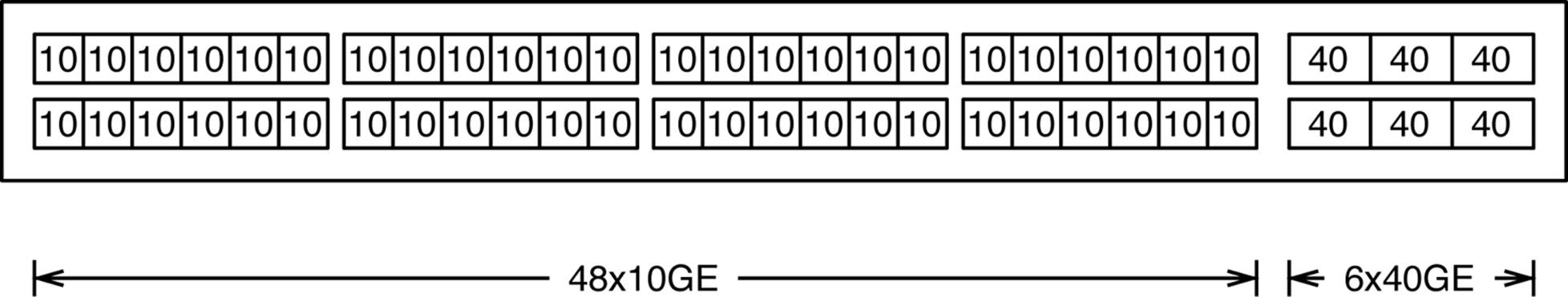
Figure 1-20. The front panel of the Juniper QFX5100-48S
In data centers where the end hosts are only 1GbE, you can change the roles of the Juniper QFX5100-48S and use it as a spine switch in the core and aggregation tiers of a data center architecture. In such a situation, you can use a lower-speed leaf such as the EX4300 in combination with the Juniper QFX5100-48S to create a spine-and-leaf topology for 1GbE access, as demonstrated in Figure 1-21.
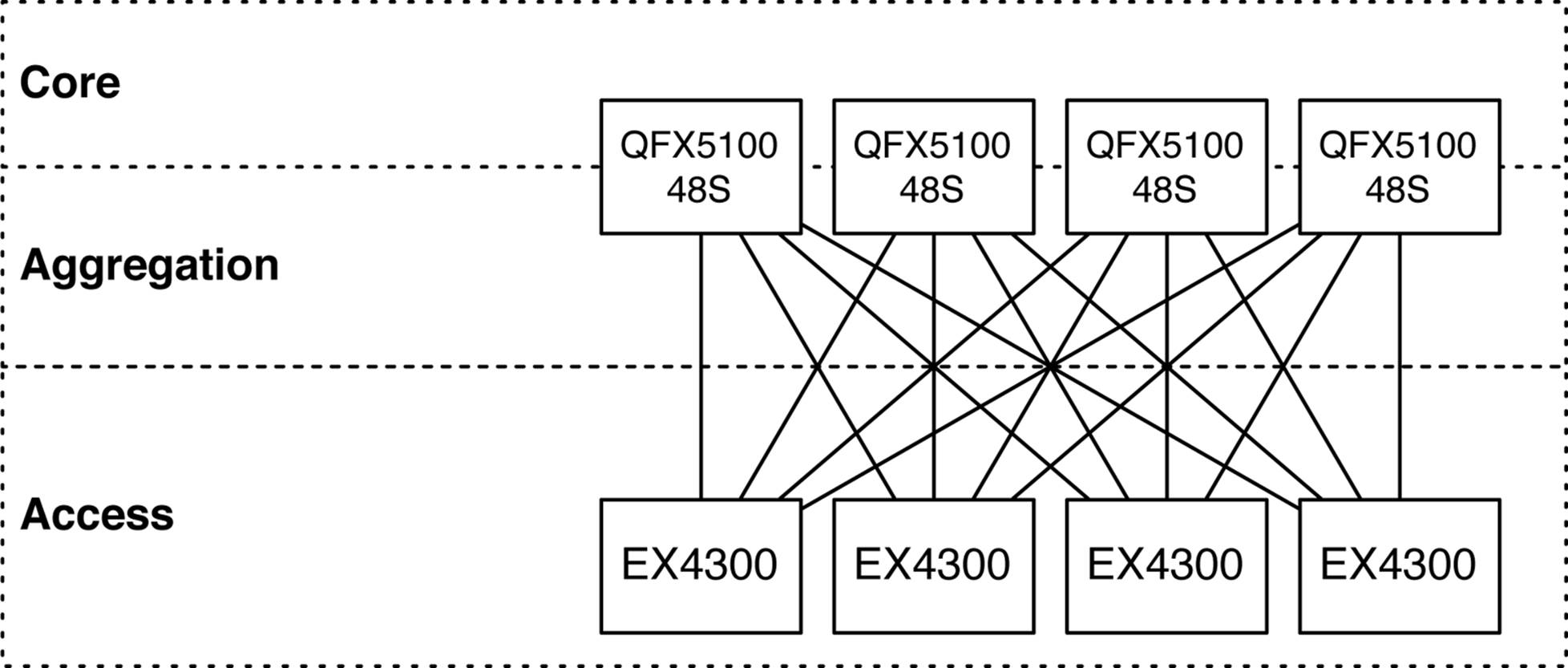
Figure 1-21. Spine-and-leaf topology with the Juniper QFX5100-48S and EX4300
The same logic holds true for a 1GbE spine-and-leaf topology: 1GbE for downstream, and 10GbE for upstream, allowing for an appropriate amount of over-subscription. In the example shown in Figure 1-21, each leaf has 4 10GbE of upstream bandwidth and 48 1GbE of downstream bandwidth; this results in an over-subscription of 1.2:1 which is nearly line rate.
Physical attributes
The Juniper QFX5100-48S is a great access switch. Table 1-5 takes a closer look at the switch’s physical attributes.
|
Physical attributes |
Value |
|
Rack units |
1 |
|
Built-in interfaces |
48 10GbE and 6 40GbE |
|
Total 10GbE interfaces |
72, using breakout cables |
|
Total 40GbE interfaces |
6 |
|
Modules |
0 |
|
Airflow |
Airflow in (AFI) or airflow out (AFO) |
|
Power |
150 |
|
Cooling |
5 fans with N + 1 redundancy |
|
PFEs |
1 |
|
Latency |
~500 nanoseconds |
|
Buffer size |
12 MB |
|
Table 1-5. Physical attributes of the QFX5100-48S |
|
Aside from the built-in interfaces and modules, the Juniper QFX5100-48S and QFX5100-24 have identical physical attributes. The key to a spine-and-leaf network is that the upstream bandwidth needs to be faster than the downstream bandwidth to ensure an appropriate level of over-subscription.
Management
Just as with the physical attributes, the Juniper QFX5100-48S and QFX5100-24Q are identical in terms of management. The Juniper QFX5100-48S has three management ports, a serial RS-232 port, and a USB port.
QFX5100-48T
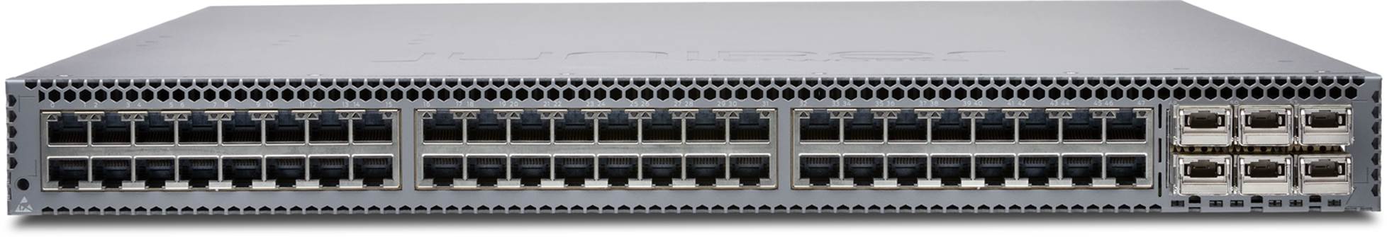
Figure 1-22. The Juniper QFX5100-48T switch
The Juniper QFX5100-48T (Figure 1-22) is very similar to the Juniper QFX5100-48S; the crucial difference is that the Juniper QFX5100-48T supports 10GBASE-T. In a data center architecture, it has been designed to fulfill the role of the access tier. In a spine-and-leaf topology, it’s most commonly used as the leaf that offers connectivity to end hosts, as shown in Figure 1-23.
Figure 1-23. Spine-and-leaf topology, with the Juniper QFX5100-48T as a leaf
Roles
The primary role for the Juniper QFX5100-48T is to operate in the access tier of a data center architecture, due to the high density of 10GbE ports. In Figure 1-23, the “L” denotes the Juniper QFX5100-48T in a spine-and-leaf topology; “S” indicates the Juniper QFX5100-24Q being used in the spine. The Juniper QFX5100-24Q and QFX5100-48T were specifically designed to work together to build a spine-and-leaf topology and offer an option of 2:1 or 3:1 over-subscription.
The front of the Juniper QFX5100-48T has two sets of built-in interfaces: 48 10GbE and 6 40GbE, as shown in Figure 1-24. The 48 10GbE interfaces are generally used for end hosts, and the 6 40GbE interfaces are used to connect to the core and aggregation. The 40GbE interfaces can also support 4 10GbE interfaces by using a breakout cable; this brings the total count of 10GbE interfaces to 72 (48 built in + 24 from breakout cables).
Figure 1-24. The front panel of the Juniper QFX5100-48T
In data centers where the end hosts are only 1GbE, the Juniper QFX5100-48T can support tri-speed interfaces:
§ 100 Mbps
§ 1 Gbps
§ 10 Gbps
The Juniper QFX5100-48T is a very flexible switch in the access layer; network operators can use the same switch for both management and production traffic. Typically, management traffic is 100 Mbps or 1 Gbps over copper by using the RJ-45 interface. New servers just coming to market in 2014 are supporting 10GBASE-T, so the Juniper QFX5100-48T can easily support both slower management traffic as well as blazingly fast production traffic.
Physical attributes
The Juniper QFX5100-48T is a great access switch. Let’s take a closer look at the switch’s physical attributes in Table 1-6.
|
Physical Attributes |
Value |
|
Rack units |
1 |
|
Built-in interfaces |
48 10GbE and 6 40GbE |
|
Total 10GbE interfaces |
48 10GBASE-T and 24 SFP+ using breakout cables |
|
Total 40GbE interfaces |
6 |
|
Modules |
0 |
|
Airflow |
Airflow in (AFI) or airflow out (AFO) |
|
Power |
150 |
|
Cooling |
5 fans with N + 1 redundancy |
|
PFEs |
1 |
|
Latency |
~500 nanoseconds |
|
Buffer size |
12 MB |
|
Table 1-6. Physical attributes of the QFX5100-48T |
|
Aside from the built-in interfaces and modules, the Juniper QFX5100-48T and QFX5100-24Q have identical physical attributes. The key to a spine-and-leaf network is that the upstream bandwidth needs to be faster than the downstream bandwidth to ensure an appropriate level of over-subscription.
Management
The management for the Juniper QFX5100-48T and QFX5100-48S are identical. The Juniper QFX5100-48T has three management ports, a serial RS-232 port, and a USB port.
QFX5100-96S
Go big or go home! The Juniper QFX5100-96S (see Figure 1-25) just happens to be my favorite switch. With 96 10GbE and 8 40GbE ports, it’s more than prepared to handle the most dense compute racks. If you don’t have enough servers in a rack to make use of this high-density switch, it also makes a great core and aggregation switch.
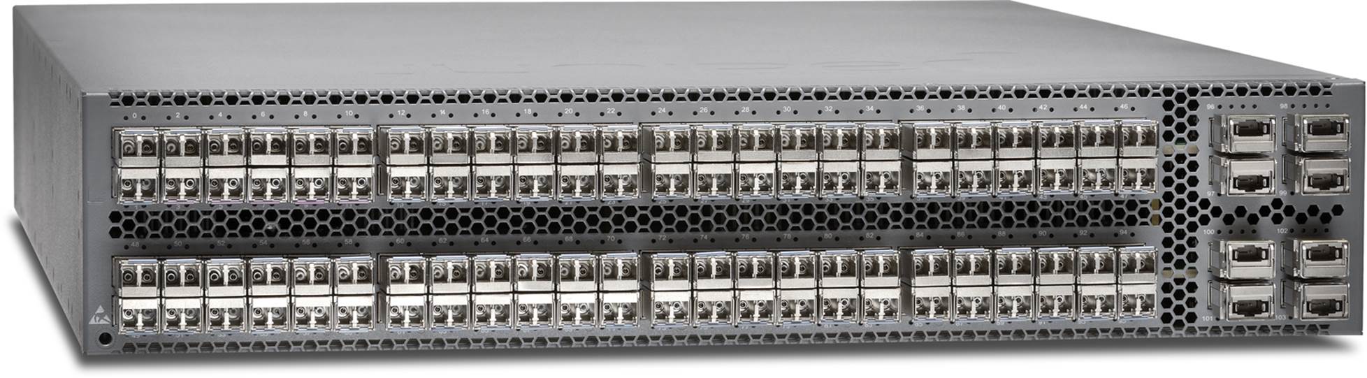
Figure 1-25. The Juniper QFX5100-96S
Roles
The Juniper QFX5100-96S is the king of access switches. As of this writing, it boasts the highest 10GbE port density in a 2RU footprint that Juniper offers. The Juniper QFX5100-96S has 96 10GbE and 8 40GbE built-in interfaces as shown in Figure 1-26.
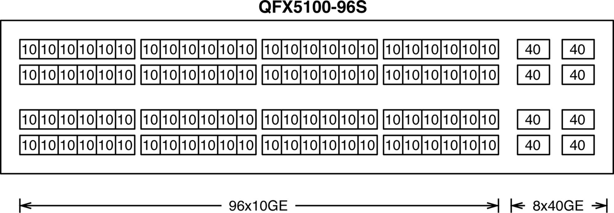
Figure 1-26. The Juniper QFX5100-96S built-in interfaces
The Juniper QFX5100-96S was specifically designed to deliver high-density 10GbE access in the largest data centers in the world, as shown in Figure 1-27; the Juniper QFX5100-96S is in the access tier denoted with an “S.”
The other option is to use the Juniper QFX5100-96S as a core and aggregation switch in the spine of the network. Using four QFX5100-96S switches in the spine will offer a dense 384 ports of 10GE.
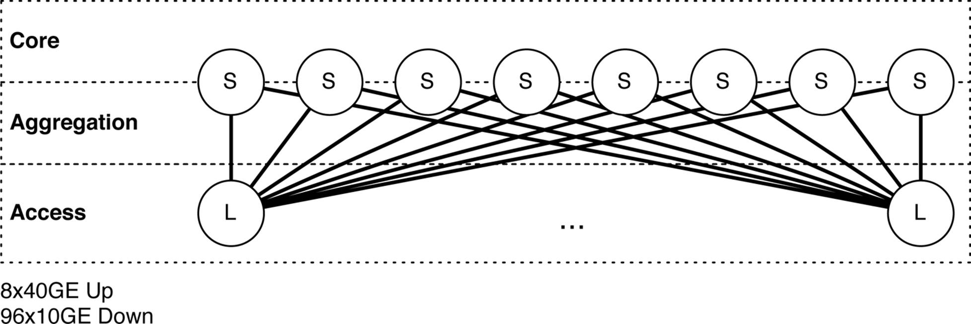
Figure 1-27. The Juniper QFX5100-96S in an access role in a spine-and-leaf topology
Physical attributes
The Juniper QFX5100-96S offers a large amount of 10GbE ports in such a small footprint. Table 1-7 lists the switch’s physical attributes.
|
Physical attributes |
Value |
|
Rack units |
2 |
|
Built-in interfaces |
96 10GbE and 8 40GbE |
|
Total 10GbE interfaces |
104 using breakout cables on two of the QSFP ports |
|
Total 40GbE interfaces |
8 |
|
Modules |
0 |
|
Airflow |
Airflow in (AFI) or airflow out (AFO) |
|
Power |
150 |
|
Cooling |
3 fans with N + 1 redundancy |
|
PFEs |
1 |
|
Latency |
~500 nanoseconds |
|
Buffer size |
12 MB |
|
Table 1-7. Physical attributes of the QFX5100-96S |
|
WARNING
Although the Juniper QFX5100-96S can physically support 128 10GbE interfaces, the BRCM 56850 chipset can only support a maximum of 104 logical interfaces.
The Juniper QFX5100-96S was modeled after the Juniper QFX5100-48S; it’s basically two QFX5100-48S switches sandwiched together. The Juniper QFX5100-96S pushes the hardware to the limit, offering the maximum amount of performance and total ports. We review the data plane in more detail later in the chapter.
Management
As with the physical attributes, the Juniper QFX5100-96S and QFX5100-48Q are identical in terms of management. The Juniper QFX5100-96S has three management ports, a serial RS-232 port, and a USB port.
Hardware Architecture
The Juniper QFX5100 family shares a lot of the same hardware to keep costs down, reduce the amount of retooling, and increase the overall reliability. The hardware is broken down into the following three major categories:
Chassis
The chassis houses all of the other components that make up the actual switch. In addition to housing the control plane and data plane, the chassis also controls the environmentals such as power and cooling.
Control Board
The control board is responsible for many management aspects of the switch. It is essentially a custom motherboard that brings together the control plane CPU, memory, solid-state disks (SSDs), I2C connections, and other management modules. The Juniper QFX5100 family uses Linux and KVM to virtualize the network operating system—Junos—which is responsible for all of the management, routing protocols, and other exception traffic in the switch.
Switch Board
The switch board brings together the built-in interfaces, expansion modules, application-specific integrated circuit (ASIC), and the precision timing module. All of the heavy lifting in terms of forwarding traffic is always processed by the data plane. Its sole purpose is to forward traffic from port to port as fast as possible.
All three components work together to bring the switch to life and make it possible for it to forward Ethernet frames in a data center. For the switch to function, all three components must be present. Given the critical nature of each component, it’s a requirement that redundancy and high availability must be a priority in the design of a switch.
Let’s take a look at the overall hardware architecture of the Juniper QFX5100 family. Each model is going to be a little different in terms of interfaces, modules, and rack units, but the major components are all the same, as is demonstrated in Figure 1-28.
Figure 1-28. Juniper QFX5100 family hardware architecture
The switch board holds together all of the components that make up the data plane; this includes all of the built-in interfaces, modules, and the Broadcom Trident II chipset. The control board houses all of the components needed to run the control plane and manage the chassis and switch board. The two power supplies are labeled as PEM0 and PEM1 (Power Entry Module). The management module is responsible for the two management interfaces, RS232 port, and USB port. Finally, the five fans in the Juniper QFX5100-24Q and QFX5100-48 are aligned in the rear of the switch so that the airflow cools the entire chassis.
Chassis
The chassis, which physically defines the shape and size of the switch, is responsible for bringing everything together. Its most important responsibility is providing power and cooling to all of the other components within it. Let’s examine each component to learn a bit more about the chassis.
Power
Each switch in the Juniper QFX5100 family requires two power supplies to support a 1 + 1 redundancy. In the event of a failure, the switch can operate on a single power supply. There are two types of power supplies: airflow in (AFI) and airflow out (AFO). The fans and power supplies must have the same airflow direction or the chassis will trigger an alarm. Each power supply is color-coded to help quickly identify the airflow direction. AFO is colored orange, and the AFI is colored blue.
Each power supply is 650 W, but the power draw is only about 280 W for a fully loaded system. On the Juniper QFX5100-96S with 96 10GbE interfaces, the average power usage is 2.9 W per 10GbE port. On the Juniper QFX5100-24Q with 32 40GbE interfaces, the average consumption is 8.7 W per 40GbE port.
Cooling
The Juniper QFX5100 family was designed specifically for the data center environment; each system supports front-to-back cooling with reversible airflow. Each chassis has a total of five fans; each fan can be either AFO or AFI. All power supplies and fans must be either AFO or AFI, otherwise the chassis will issue alarms.
Sensors
Each chassis has a minimum of seven temperature sensors, whereas chassis that support modules have a total of nine sensors. This is so each module has its own temperature sensor. Each sensor has a set of configurable thresholds that can raise a warning alarm or shutdown the switch. For example if the CPU were running at 86° C, the switch would sound a warning alarm; however, if the temperate were to rise to 92° C, it would shut down the system to prevent damage.
If you want to see what the current temperatures and fan speeds are, use the show chassis environment command, as shown in the following:
dhanks@opus> show chassis environment
Class Item Status Measurement
Power FPC 0 Power Supply 0 OK
FPC 0 Power Supply 1 OK
Temp FPC 0 Sensor TopMiddle E OK 29 degrees C / 84 degrees F
FPC 0 Sensor TopRight I OK 24 degrees C / 75 degrees F
FPC 0 Sensor TopLeft I OK 27 degrees C / 80 degrees F
FPC 0 Sensor TopRight E OK 25 degrees C / 77 degrees F
FPC 0 Sensor CPURight I OK 30 degrees C / 86 degrees F
FPC 0 Sensor CPULeft I OK 28 degrees C / 82 degrees F
FPC 0 Sensor CPU Die Temp OK 45 degrees C / 113 degrees F
Fans FPC 0 Fan Tray 0 OK Spinning at normal speed
FPC 0 Fan Tray 1 OK Spinning at normal speed
FPC 0 Fan Tray 2 OK Spinning at normal speed
FPC 0 Fan Tray 3 OK Spinning at normal speed
FPC 0 Fan Tray 4 OK Spinning at normal speed
To view the default thresholds, use the show chassis temperature-thresholds commands, as demonstrated here:
dhanks@opus> show chassis temperature-thresholds
Fan speed Yellow alarm Red alarm Fire Shutdown
(degrees C) (degrees C) (degrees C) (degrees C)
Item Normal High Normal Bad fan Normal Bad fan Normal
FPC 3 Sensor TopMiddle E 47 67 65 65 71 71
FPC 3 Sensor TopRight I 41 65 63 63 69 69
FPC 3 Sensor TopLeft I 45 67 64 64 70 70
FPC 3 Sensor TopRight E 42 64 62 62 68 68
FPC 3 Sensor CPURight I 40 67 65 65 71 71
FPC 3 Sensor CPULeft I 44 65 63 63 69 69
FPC 3 Sensor CPU Die Temp 62 93 86 86 92 92
It’s important that you review the default sensor thresholds and see if they’re appropriate for your environment; they’re your insurance policy against physically damaging the switch in harsh environments.
Control Plane
The control plane is essentially the brain of the switch. It encompasses a wide variety of responsibilities that can be broken down into the following four categories:
Management
There are various ways to manage a switch. Some common examples are SSH, Telnet, SNMP, and NETCONF.
Configuration and Provisioning
There are tools and protocols to change the way the switch operates and modify state. Some examples include Puppet, Chef, Device Management Interface (DMI), Open vSwitch Database (OVSDB), and OpenFlow.
Routing Protocols
For a switch to participate in a network topology, it’s common that the switch needs to run a routing protocol. Some examples include OSPF, IS-IS, and BGP.
Switching Protocols
The same goes for Layer 2 protocols, such as LLDP, STP, LACP, and MC-LAG.
As described earlier in the chapter, Junos, the network operating system, is responsible for all of the preceding functions.
The Juniper QFX5100 has a little trick up its sleeve. It takes virtualization to heart and uses Linux and KVM to create its own virtualization framework (see Figure 1-30). This creates two immediate benefits:
Two Routing Engines
Even though the control board has a single dual-core CPU, taking advantage of virtualization, the Juniper QFX5100 is able to have two routing engines. One of the primary benefits of two routing engines is the set of high-availability features. The Juniper QFX5100 is able to take full advantage of Nonstop Routing (NSR), Nonstop Bridging (NSB), Graceful Routing Engine Failover (GRES), and In-Service Software Upgrade (ISSU).
Snapshots
One of the great aspects of hypervisors is that they can take a snapshot of a virtual machine and have the ability to revert back to a snapshot at any time. Do you have a big upgrade planned? Need a backout plan? Snapshots to the rescue.
Let’s take a look at how the Juniper QFX5100 is able to virtualize the control plane. Figure 1-29 shows that the main tool being used is Linux and KVM.
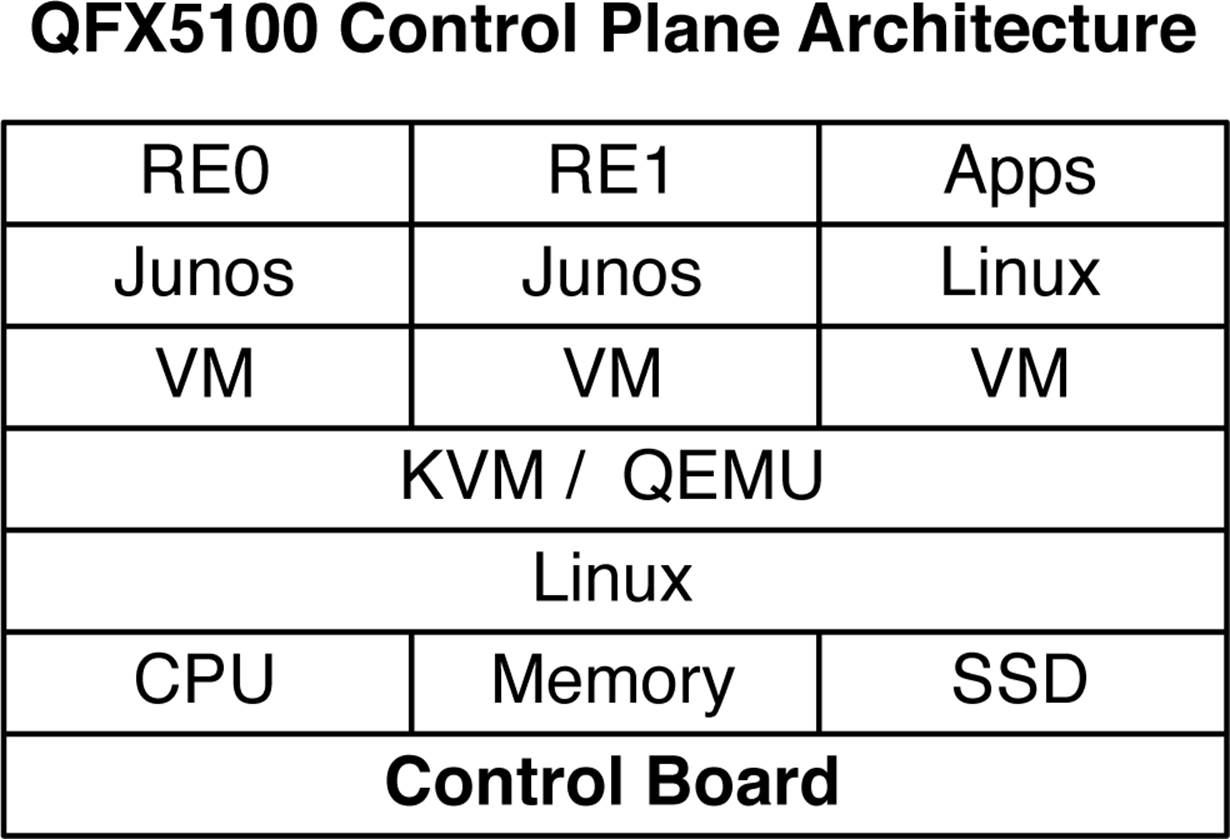
Figure 1-29. The Juniper QFX5100 control plane architecture
The Juniper QFX5100 is able to reap all of the high-availability benefits through virtualization that are usually reserved for high-end systems such as the Juniper MX and T Series. In addition to having two routing engines, there’s enough space remaining to have a third virtual machine that you can use for third-party applications. Perhaps you have some management scripts that need to be hosted locally, and you don’t want it to interfere with the switch’s control plane. No problem, there’s a VM for that.
NOTE
Are you interested in control plane virtualization and want to learn more? Chapter 2 is dedicated to just that and shows you how all of this works and is put together.
Processor, memory, and storage
The Juniper QFX5100 uses a modern Intel dual-core CPU based on the Sandy Bridge architecture. The processor speed is 1.5 GHz, which is more than adequate for two routing engines and third-party applications. The control board has 8 GB of memory. Finally, the control board has a pair of 16 GB high-speed SSDs. Overall the Juniper QFX5100 has a really zippy control plane, and you will enjoy the fast commit times and quickness of the Junos CLI.
Data Plane
So, let’s get right to it. The data plane is driven by a Broadcom BCM56850 chipset, which is also known as the Trident II. As of this writing, it’s one of the latest 10/40GbE chipsets on the market from Broadcom. The Trident II chipset brings many great features of which you can take advantage:
Single Chipset
Switch on a Chip (SoC) is a concept whereby the entire data plane of a switch is driven by a single chipset. The advantage of this architecture is that it offers much lower latency as compared to multiple chipsets. The Trident II chipset has enough ports and throughput to drive the entire switch.
Overlay Networking
With the rise of SDN, new protocols such as VXLAN and NVGRE are being used to decouple the network from the physical hardware. The Trident II chipset supports the tunnel termination of both VXLAN and NVGRE in hardware with no performance loss.
Bigger, Better, Faster
The Trident II chipset has more ports, more bandwidth, and higher throughput; this allows the creation of better switches that can support a wide variety of port configurations. Creating a family of switches that can be deployed in multiple roles within a data center architecture using the same chipset has many advantages for both the customer and vendor.
Merchant silicon
Chipsets such as the Broadcom Trident II are often referred to as merchant silicon or “off-the-shelf silicon” (OTS). Many networking vendors offer similar networking switches that are based off the same chipsets as the Trident II. It would be an incorrect assumption that networking switches that are based on the same chipsets are identical in function. Recall from Figure 1-28, that the architecture of a network switch includes three primary components: the chassis, switch board, and control board. The control plane (control board) and the data plane (switch board) must both be programmed and synchronized in order to provide a networking service or feature. In other words, although the chipset might support a specific feature, unless the control plane also supports it, you won’t be able to take advantage of it. Given the importance of the control plane, it becomes increasingly critical when comparing different network switches.
Having casual knowledge of the various chipsets helps when you need to quickly access the “speeds and feeds” of a particular network switch. For example, network switches based on the Trident II chipset will generally support 10GbE and 40GbE interfaces, allow up to 104 interfaces, and will not exceed 1,280 Gbps of overall throughput. Such limitations exist because it’s the inherent limitation of the underlying chipset used in the network switch.
It’s absolutely required that both the control plane and data plane support a particular network feature or service in order for that service or switch to be usable. Sometimes network vendors state that a switch is “Foobar Enabled” or “Foobar Ready,” which merely hints that the chipset itself supports it, but the control plane doesn’t and requires additional development. If the vendor is being extra tricky, you will see “Foobar*,” with the asterisk denoting that the feature will be released—via the control plane—in the future.
The control plane really brings the network switch to life; it’s the brains behind the entire switch. Without the control plane, the switch is just a piece of metal and silicon. This poses an interesting question: if multiple network vendors use the same chipsets in the data plane, how do you choose which one is the best for your network? The answer is simple and has two sides: the first is the switch board flexibility, and the second is the differentiation that comes through the control plane.
Even though the chipset might be the same, vendors aren’t limited in how they can use it to create a switch. For example, using the same chipset, you could build a fixed-port network switch or create a network switch that uses modules. Some configurations make sense such as the 48 10GbE, because this is a common footprint for a compute rack. There are other use cases besides an access switch; having the flexibility to use different modules in the same switch allows you to place the same switch in multiple roles in a data center.
More than any other component, the control plane impacts what is and what isn’t possible with a network switch that’s based off merchant silicon. Some vendors limit the number of data center technologies that are enabled on the switch. For example, you can only use the switch in an Ethernet fabric or it only supports features to build a spine-and-leaf network. Right off the bat, the control plane has already limited where you can and cannot use the switch. What do you do when you want to build an Ethernet fabric, but the switch can only be used in a spine-and-leaf network? The Juniper QFX5100 family is known for “one box, many options” because it offers six different switching technologies to build a network. You can read more about these technologies in Chapter 3.
There are many inherent benefits that come with virtualizing the control plane by using a hypervisor. One is the ability to create snapshots and roll back to a previous known-good state. Another is the ability to have multiple control planes and routing engines to enable features such as ISSU with which you can upgrade the switch without dropping any traffic.
The control plane makes or breaks the switch. It’s crucial that you’re familiar with the features and capabilities of the networking operating system. Junos has a very strong pedigree in the networking world and has been developed over the past 15 years, which results in a very stable, robust, and feature-rich control plane. The control plane is so critical that part of this chapter is dedicated to the Junos architecture, and Chapter 2 focuses directly on the control plane virtualization architecture.
Architecture
So, let’s consider the Trident II chipset architecture. First and foremost is that the Trident II has enough throughput and supports enough logical ports that it can drive the entire network switch itself. Using a single chipset enables an SoC design that lowers the overall power consumption and port-to-port latency. The Trident II chipset has eight primary engines, as depicted in Figure 1-30.
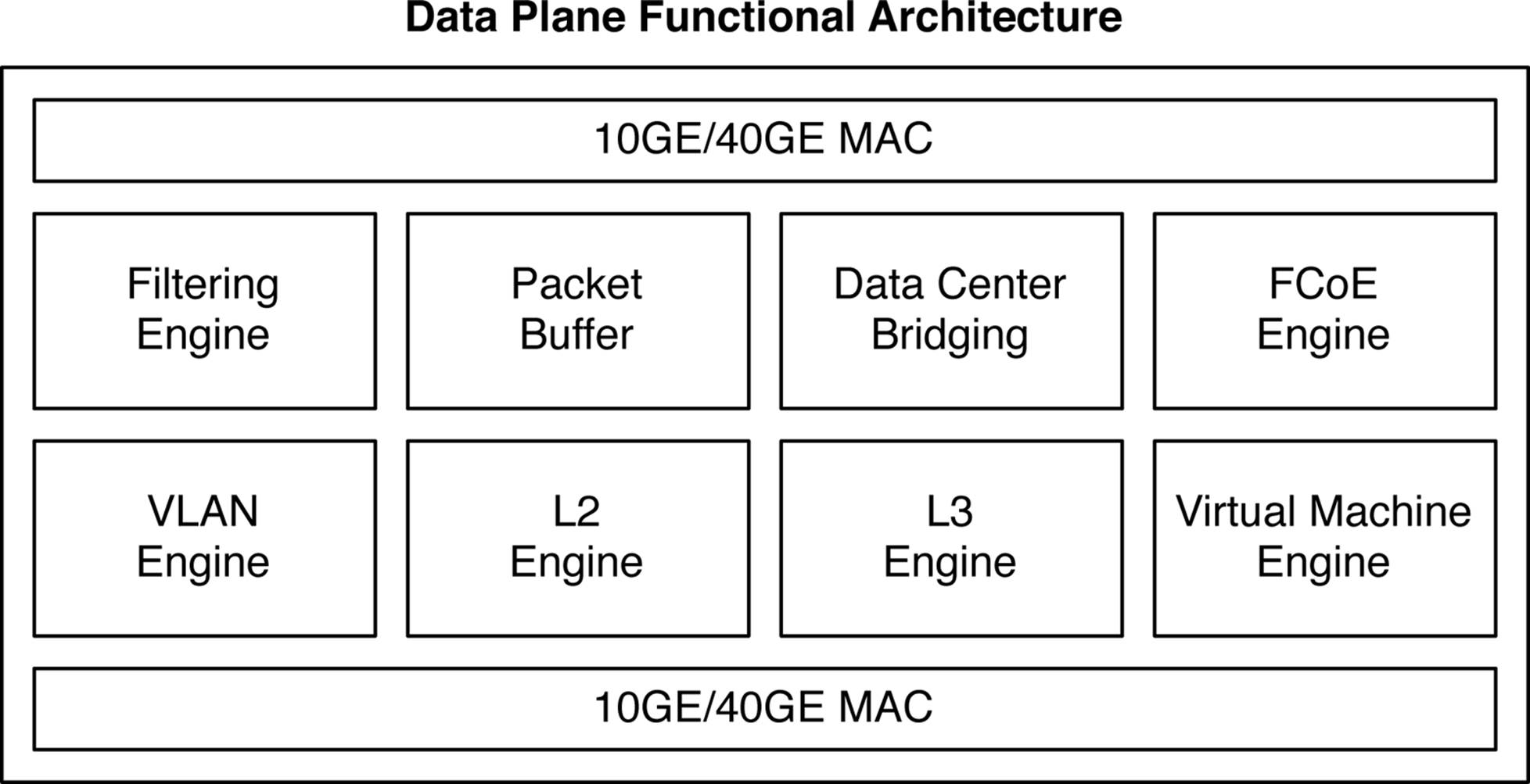
Figure 1-30. Data plane functional architecture
Data is handled by the 10GbE and 40GbE interfaces and is processed by the eight internal traffic engines. Each engine represents a discrete step in processing each Ethernet frame that flows through the switch. By looking at the available functions of a chipset, you can make some immediate assumptions regarding where the chipset can be used in the network. For example, the chipset functions in Figure 1-30 are appropriate for a data center or campus network, but they wouldn’t be applicable for an edge and aggregation network or optical-core network. You have to use a chipset with the appropriate functions that match the role in the network; this is why vendors use merchant silicon for some devices and custom silicon for others, depending on the use case.
Life of a frame
As an Ethernet frame makes its way from one port to another, it has to move through different processing engines in the data plane, as shown in Figure 1-31.
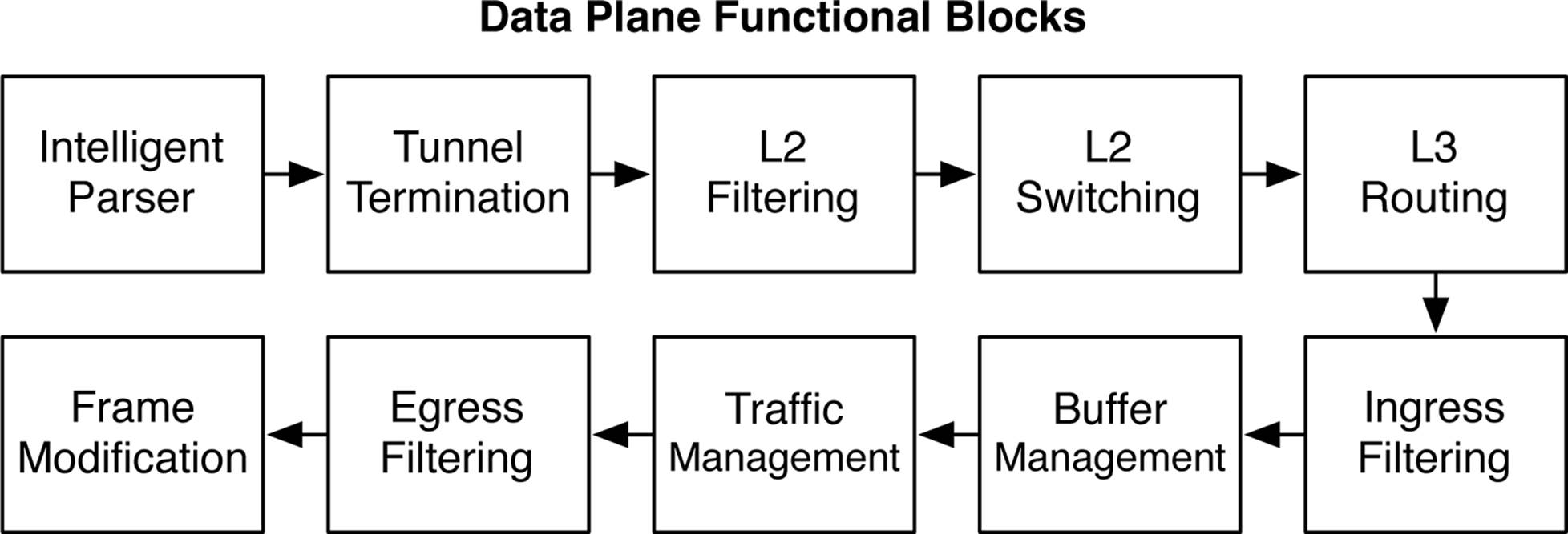
Figure 1-31. Data plane function blocks
Each functional block makes modifications to the Ethernet frame and then passes it to the next functional block in the workflow. Each functional block has a very specific function and role in processing the Ethernet frame. The end result is that as an Ethernet packet flows through the switch, it’s able to be manipulated by a wide variety of services without a loss of performance. The following are descriptions of each functional block:
Intelligent Parser
The first step is to parse the first 128 bytes of the Ethernet frame. Various information, such as the Layer 2 header, Ethernet Type, Layer 3 header, and protocols are saved into memory so that other functional blocks can quickly access this information.
Tunnel Termination
The next step is to inspect the Ethernet frame in more detail and determine if the switch needs to be a termination point of any tunnel protocols, such as VXLAN, GRE, and MPLS.
Layer 2 Filtering
This functional block is a preprocessor to determine where to route Layer 2 and Layer 3 packets. During this phase the packet can be moved to a different VLAN or VRF depending on the information in the first 128 bytes.
Layer 2 Switching
During this stage of the process, the switch needs to process all Layer 2 functions such as VLAN switching, process double-tags, and process encapsulations such as GRE, MPLS, or VXLAN.
Layer 3 Routing
When all of the Layer 2 processing is complete, the next stage in the process is Layer 3. The Layer 3 routing functional block is responsible for unicast and multicast lookups, longest prefix matching, and unicast reverse path forwarding (uRPF).
Ingress Filtering
The most powerful filtering happens in the ingress filtering functional block. The filtering happens in two stages: match and action. Nearly any field in the first 128 bytes of the packet can be used to identify and match fields that should be subject to further processing. The actions could be to permit, drop, or change the forwarding class, or assign a new next hop.
Buffer Management
All Quality of Service features, such as congestion management, classification, queuing, and scheduling are performed in the buffer management functional block.
Traffic Management
If the Ethernet frame is subject to hashing such as LACP or ECMP, the packet is run through the hashing algorithm to select the appropriate next hop. Support for storm control for broadcast, multicast, and unknown unicast (BUM) is managed by the traffic management functional block.
Egress Filtering
Sometimes, it’s desirable to filter packets on egress. The egress filtering functional block is identical to the ingress filtering functional block, except that the matching and actions are performed only for egress packets.
Frame Modification
Depending on all of the prior processing of the Ethernet frame, the final egress frame might require substantial modification. In the simplest form the switch can merely just decrement the IP time-to-live (TTL). A more complicated example would be that an Ethernet frame needs to be encapsulated with VXLAN or MPLS.
In summary, there are 10 discrete functional blocks that have specific roles and responsibilities. Starting with intelligent parsing and ending with frame modification, the life of a frame is subject to an end-to-end workload. Separating out the functions into different blocks facilitates predictable behavior and latency as the Ethernet frame makes its way through the switch.
Design Options
Let’s take a look at some of the most common design options, and understand what the differences are between them, and what challenges they solve. The following design options will only make use of the Juniper QFX5100 family platforms. There are other design options that can include QFabric and other platforms, but we will review these in detail later in the book.
768×10GbE Ethernet Fabric
The first and most common design option is to create an Ethernet fabric using the Juniper QFX5100 family. The Ethernet fabric—the VCF—is able to provide a single point of management, 3:1 over-subscription, and FCoE support. VCF will be covered in detail in Chapter 6, but let’s take a sneak peek at the topology and design benefits.
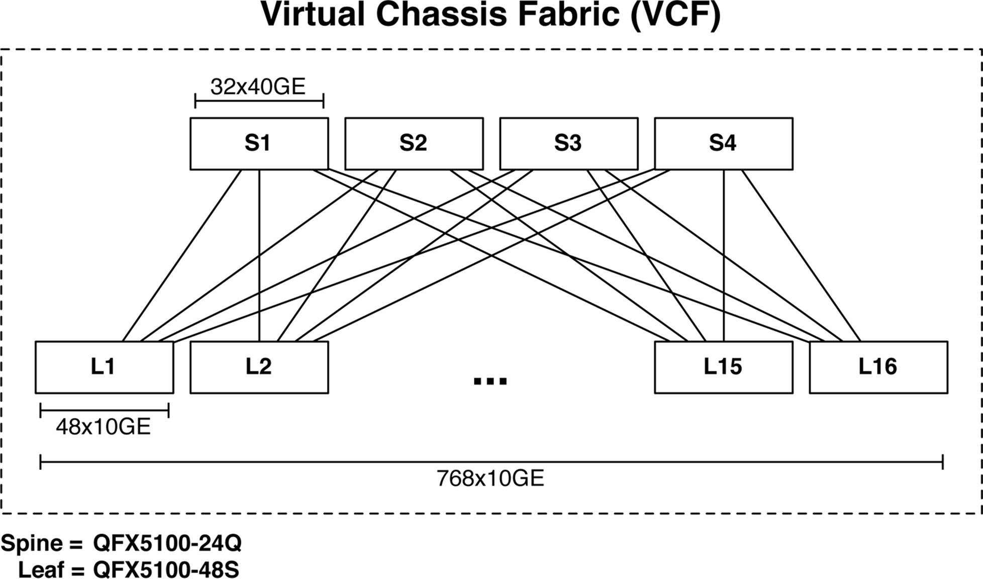
Figure 1-32. 768 10GbE VCF
As of this writing, a VCF has only two rules:
§ The number of spines cannot exceed four members.
§ The total number of switches in the fabric cannot exceed 20 members.
The example in Figure 1-32 has four spines using the Juniper QFX5100-24Q and 16 leaves using the Juniper QFX5100-48S; the total number of switches in this design option is 20. Each spine has 32 40GbE interfaces, and each leaf has 48 10GbE and 6 40GbE interfaces. Each leaf is using only 4 40GbE interfaces to connect to the spine, so the total over-subscription is 480:160 or 3:1.
NOTE
The astute reader will realize that only 4 out of the 6 40GbE interfaces on the Juniper QFX5100-48S is being used. In addition, there are only 16 out of 32 40GbE interfaces being used on the Juniper QFX5100-24Q in the spine. This is because of the current limitation of 20 devices in a VCF.
Building a VCF with 768 10GbE interfaces is perfect for many small to medium-sized data centers. Let’s explore the benefits of this VCF design option:
§ 768 10GbE ports
§ Single point of management and control
§ Full support for FCoE and converged storage
§ Topology-independent ISSU
§ Full ECMP for both Layer 2 and Layer 3
§ Plug-and-play implementation
§ In-band control plane with no additional equipment required
§ 1.5 µs end-to-end latency
With the assumption that each server requires two 10GbE links, a VCF network is a great way to easily manage 384 servers with a single Ethernet fabric that supports converged storage and the ability to upgrade the software without traffic loss. Also, assume that each server can support up to 20 VMs; VCF can support 384 servers and 7,680 VMs.
3,072 10GbE Clos
A common alternative to building a Virtual Chassis Fabric is to build a Layer 3 Clos Fabric, as illustrated in Figure 1-33. One of the key benefits of a Clos fabric is the large scale; in this example, the Clos fabric is able to scale up to 3,072 10GbE ports.
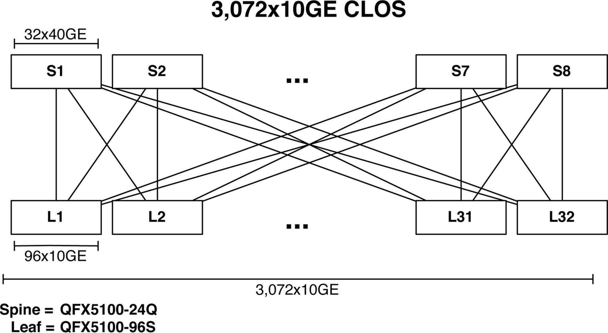
Figure 1-33. 3,072 10GbE Clos fabric
Clos fabrics are covered in greater depth in Chapter 8, but let’s take a look at some of the key features of this design option. The speed and number of uplink interfaces of the leaf switch determine the shape and size of the spine. In Figure 1-33, the leaf switch is the Juniper QFX5100-96S, which has 8 40GbE uplinks. To build a simple Clos, the easiest option is to select a spine switch that supports 40GbE interfaces and have eight of them, which matches the number of uplinks on the Juniper QFX5100-96S. In this example, we’ll use the Juniper QFX5100-24Q in the spine, which results in a total of 32 40GbE interfaces. With a total of eight spine switches, this results in 256 40GbE interfaces that can be used by the leaf switches. Because each QFX5100-96S has eight uplinks, we’ll have a total of 32 leaves (256 ports/8 uplinks = 32 leaves). Each leaf has 96 10GbE interfaces, thus the Clos fabric has 3,072 10GbE interfaces (96 ports × 32 leaves = 3,072 10GbE).
One of the central assumptions with a Layer 3 Clos is that each switch uses a routing protocol such as OSPF, IS-IS, or BGP to connect to one another. If you have a virtualized workload and want to use an overlay architecture, a Layer 3 Clos is the perfect way to scale out your data center.
12,288 10GbE Clos
Now that you’re familiar with a Layer 3 Clos, let’s take it to the next level. The key to building a large Clos is the number of ports that are available in the spine. An easy way to increase the number of ports in the spine is to use VCF, as illustrated in Figure 1-34.
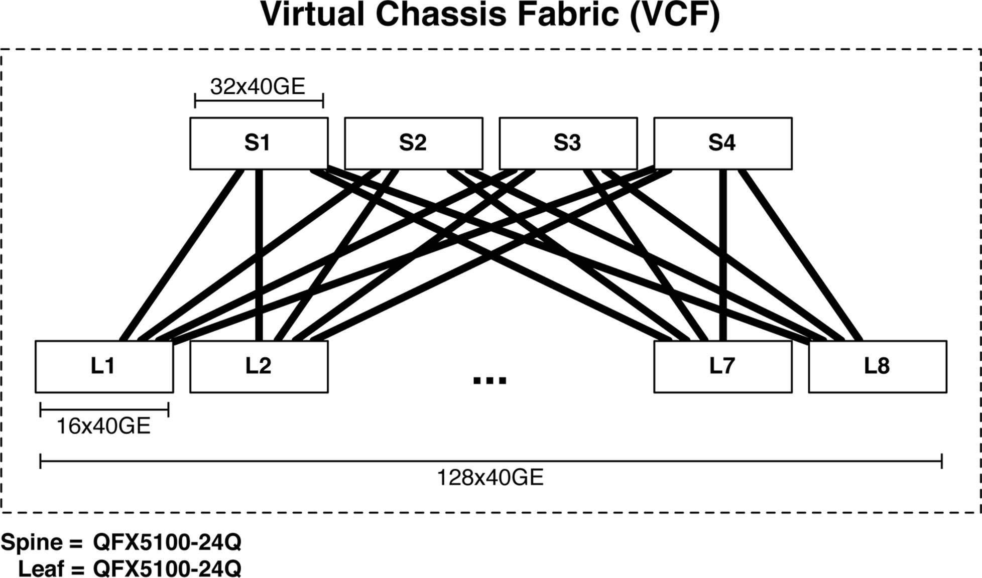
Figure 1-34. 128 40GbE VCF with 1:1 over-subscription
Using the 128 40GbE VCF illustrated in Figure 1-34, we’ve increased the capacity of a single spine switch from 32 to 128. Now, let’s use the 128 40GbE VCF as a spine switch in a Clos fabric, as shown in Figure 1-35.
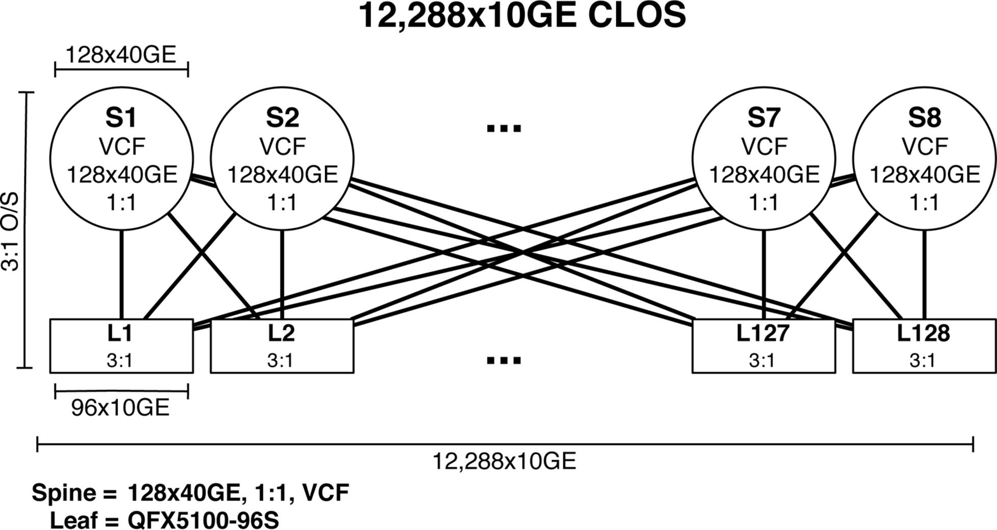
Figure 1-35. 12,288 10GbE Clos fabric
Something very interesting just happened in this design option: we’ve used a “feature within a feature” or a hierarchical approach. Typically, most people confine their thinking to a single physical switch when identifying a spine switch. If you take a look at the requirements of a spine switch, it’s fairly basic:
§ Generally 1:1 over-subscription
§ Generally 40GbE interfaces
§ Single point of management
§ Capable of Layer 3
It’s true that a single physical switch meets the above requirements, but so does VCF. In the example in Figure 1-35 the spine switches are VCF fabrics. Each VCF spine has four QFX5100-24Q switches in its spine and eight QFX5100-24Q switches in its leaves; this gives a total of 128 40GbE interfaces at 1:1 over-subscription. To meet the 1:1 over-subscription requirement, each leaf has 16 40GbE down and 16 40GbE going up to the spine. Four spine switches handling 16×40GbE interfaces from each leaf can result in 8 leaves total (4 spines × 32 ports)/16 uplinks = 8 leaves. We can summarize the spines S1 through S8 in Figure 1-35 as follows:
§ (4) QFX5100-24Q switches in the spine.
§ (8) QFX5100-24-Q switches as the leaves.
§ 16 40GbE interfaces going up to the spine.
§ 16 40GbE interfaces available for use.
§ 12 switches total in the VCF.
§ 128 40GbE usable interfaces.
§ 1:1 over-subscription.
The 12,288 10GbE design option has 138 discrete points of management; the assumption is that each VCF is a point of management (8) as well as of all the leaves (128). Here’s a summary of the benefits of the Clos fabric:
§ 12,288 10GbE ports
§ No traffic loss during software upgrades with topology-independent ISSU
§ Spine switches are a single point of management through VCF
§ 3:1 over-subscription
§ 2.5 µs end-to-end latency
§ Lossless Ethernet support with PFC over Layer 3
Building a Clos is a great way to easily scale the network in an overlay architecture or in environments that don’t require Layer 2 between leaves.
49,152 10GbE Clos
So, let’s step up the game a little bit. Let’s assume that we don’t need a single point of management in the spine. How would this effect the scale of the network? Let’s first start by building the largest 40GbE Clos spine we can with the Juniper QFX5100-24Q, assuming 1:1 over-subscription, as shown in Figure 1-36.
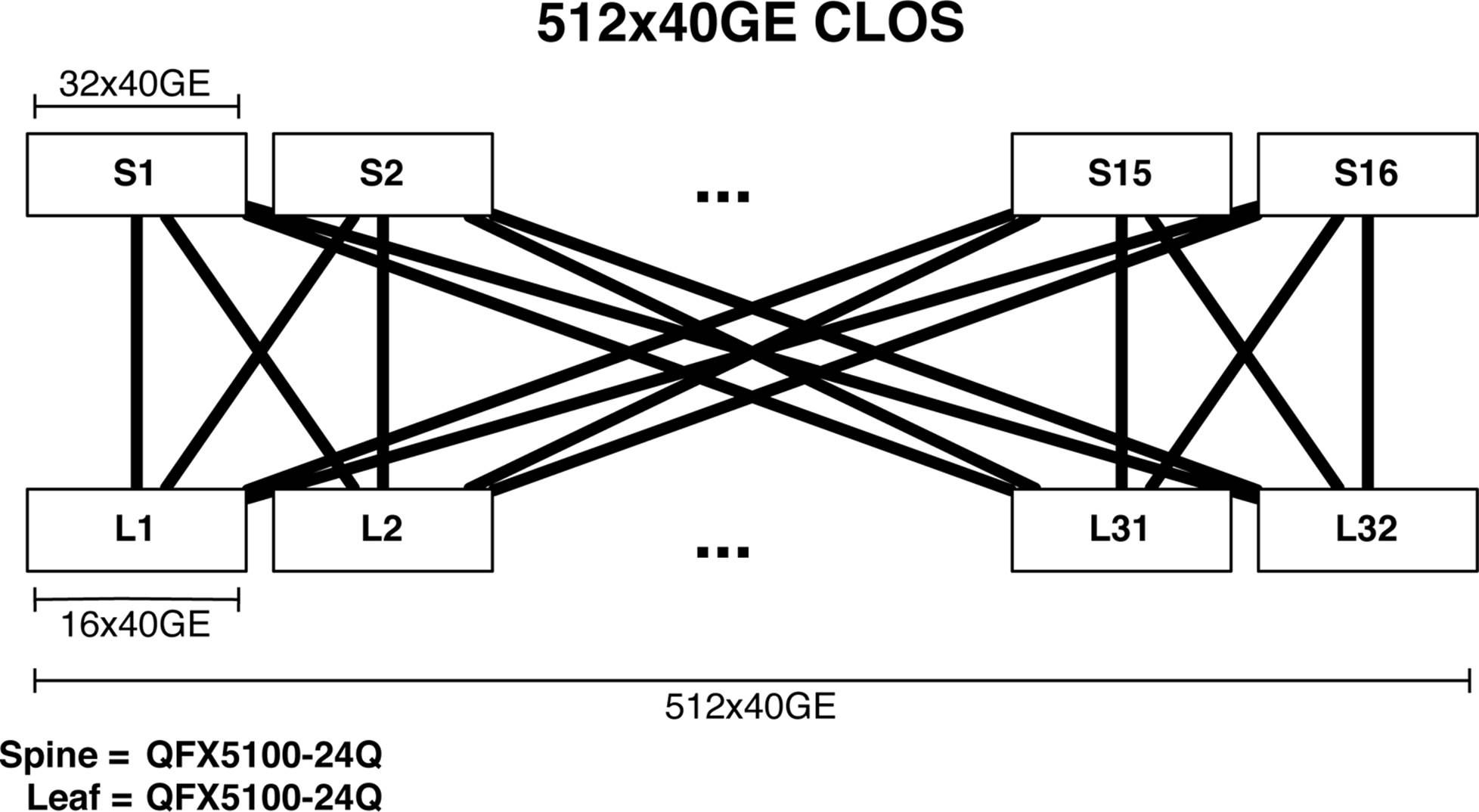
Figure 1-36. 512 40GbE Clos with 1:1 over-subscription
Now, each spine node can be a 512 40GbE Clos. This is the same concept as using VCF, but in this case, each switch in the Clos has to be managed separately; this type of design is referred as a Clos within a Clos.
NOTE
<meme>Yo dawg, I herd you like Clos, so I put a Clos in your Clos so you can Clos while you Clos</meme>
With each spine supporting 512 40GbE interfaces, we can combine it with the Juniper QFX5100-96S switch, which has 8 40GbE uplinks. 512 ports × 8 spines / 8 uplinks = 512 leaves; finally 512 leaves × 96 ports = 49,152 10GbE ports, as illustrated in Figure 1-37.

Figure 1-37. 49,152 10GbE Clos fabric
The end result is that we have a very large Clos fabric that supports 49,152 10GbE ports. Let’s take a moment to review the benefits of the Clos fabric:
§ 49,152 10GbE ports
§ No traffic loss during software upgrades with topology-independent ISSU
§ 3:1 over-subscription
§ 2.5 µs end-to-end latency
§ Lossless Ethernet support with PFC over Layer 3
One of the main assumptions to a Clos fabric of this size is that it operates at Layer 3; thus, your infrastructure and servers must not be dependent on Layer 2. Examples of such applications and infrastructure are web applications, Platform as a Service (PaaS), and overlay architecture. Keeping things simple at a large scale will reduce the amount of things that can go wrong. Layer 3 has very fast convergence, is loop free, and is able to scale easily.
Summary
This chapter has covered a lot of topics ranging from software to hardware. It’s important to understand how the software and hardware are designed to work in conjunction with each other. This combination creates a best-in-class switch that is able to solve the difficult challenges data center operators are facing with the explosion of high-density 10GbE server ports and the need for delivering network services within seconds.
Being specifically designed to solve cloud computing and SDN requirements, the Juniper QFX5100 family solves a wide variety of challenges and offers many unique benefits, including the following:
Transport
Dense 10GbE and 40GbE interfaces to build a deterministic spine-and-leaf topology with an option of 1:1, 3:1, or 6:1 over-subscription.
Interfaces
Each 10GbE interface is tri-speed and supports 100 Mbps, 1GbE, or 10GbE. In addition, each interface can support either copper or fiber connectivity. Higher interface speeds such as 40GbE can be broken out into 4 10GbE interfaces by using a breakout cable.
Overlay Networking
Each switch offers complete integration with Contrail and NSX to support overlay networking. You can configure the Juniper QFX5100 family as the end point in an overlay network architecture to support bare-metal servers.
Latency
An intelligent algorithm is used for each ingress packet to determine which forwarding architecture—store-and-forward or cut-through—should be used to guarantee the least latency. On average, the port-to-port latency is only 500 nanoseconds.
Flexible Deployment Options
The Juniper QFX5100 series doesn’t force you into deploying a particular technology or proprietary protocol. The Juniper QFX5100 family supports standalone, Virtual Chassis, QFabric node, VCF, MC-LAG, or a Clos architecture.
QFabric Node
You can use the Juniper QFX5100 as a node in the QFabric architecture. All of the benefits of the Juniper QFX5100 are available when used as a QFabric node: higher port density, overlay networking, and lower latency.
Virtualized Control Plane
The Juniper QFX5100 takes virtualization to heart. The control plane uses an Intel Sandy Bridge CPU. The host operating system is Linux running KVM and QEMU for virtualization. The network operating system is Junos and runs as a VM and is able to take advantage of all of the benefits of virtualization such as ISSU.
Unified Forwarding Table
Whether you need to support more MAC addresses or IPv4 prefixes in a Clos architecture, the Juniper QFX5100 allows you to adjust the profile of the forwarding table. There are five preconfigured profiles that range from L2 heavy to L3 heavy.
Network Analytics
Some applications are sensitive to microbursts and latency. The Juniper QFX5100 makes it possible for you to get on-box reporting of queue depth, queue latency, and microburst detection to facilitate and speed up the troubleshooting process.
Lossless Ethernet
When converging storage and data, it’s critical that storage be handled in such a way that no traffic is dropped. The Juniper QFX5100 family supports DCBX, ETS, and PFC to enable transit FCoE or lossless Ethernet for IP storage.
VCF
Ethernet fabrics provide the benefit of a single point of management, lossless Ethernet, and full Layer 2 and Layer 3 services. The Juniper QFX5100 series can form a VCF Ethernet fabric. This is a spine-and-leaf topology that supports full ECMP but with all of the benefits of an Ethernet fabric.
Inline Network Services
Traditionally network services such as GRE and NAT are handled by another device such as a router or firewall. The Juniper QFX5100 family can perform both GRE and NAT in hardware without a performance loss.
The Juniper QFX5100 family brings a lot new features and differentiation to the table when it comes to solving data center challenges. Because of the wide variety of features and differentiation, the Juniper QFX5100 is able to be positioned into many different types of architectures, such as the following:
High-Frequency Trading
Speed is king when it comes to trading stocks; with an average port-to-port latency of 500 nanoseconds, the Juniper QFX5100 family fits well in a high-frequency trading architecture.
Private Cloud
Although the Juniper QFX5100 was specifically designed to solve the challenges of cloud computing and public clouds, you can use the same features to solve the needs of the private cloud. Enterprises, government agencies, and research institutes are building out their own private clouds, and the Juniper QFX5100 meets and exceeds all requirements.
Campus
High port density and a single point of management make the Juniper QFX5100 series a perfect fit in a campus architecture, specifically in the core and aggregation roles.
Enterprise
Offering the flexibility to be used in multiple deployment scenarios, the Juniper QFX5100 family gives the enterprise the freedom to use the technology that best fits its needs. You can use it as a standalone device, Virtual Chassis, QFabric Node, VCF, MC-LAG, or in a Clos architecture.
It’s a very exciting time in the networking industry as SDN, cloud computing, and data center technologies are continuing to push the envelope and bring new innovations and solutions to the field. The Juniper QFX5100 series of switches is embracing all of the change that’s happening in the networking industry and providing clear and distinctive solution differentiation. With its wide variety of features and differentiation, the Juniper QFX5100 family is able to quickly solve the challenges of cloud computing in the data center as well as other use cases such as high-frequency trading and high-performance computing.
Chapter Review Questions
1. Which version of Junos is supported for three years?
1. The first major release of the year
2. The last maintenance release of the year
3. The last major release of the year
4. The last service release of the year
2. Which is not a function of the control plane?
1. Processing SSH traffic destined to the router
2. Updating the RIB
3. Updating the FIB
4. Processing a firewall filter on interface xe-0/0/0.0
3. How many modules does the Juniper QFX5100-24Q have?
1. 1
2. 2
3. 3
4. 4
4. Which functional block processes congestion management?
1. Intelligent parser
2. Traffic management
3. Buffer management
4. Frame modification
5. What hypervisor does the Juniper QFX5100 use for the control plane?
1. Microsoft Hyper-V
2. VMware ESXi
3. Linux KVM
4. Linux Containers
6. On what chipset is the Juniper QFX5100 based?
1. Broadcom Trident
2. Broadcom Trident II
3. Marvell Lion
4. Juniper Trio
7. On what tier in the network does the Juniper QFX5100 support ISSU?
1. Core
2. Aggregation
3. Access
4. All
Chapter Review Answers
1. Answer: C.
The last major release of Junos of a given calendar year is known as the Extended End of Life (EEOL) release and is supported for three years.
2. Answer: D.
The data/forwarding plane handles all packet processing such as firewall filters, policers, or counters on the interface xe-0/0/0.0.
3. Answer: B.
The Juniper QFX5100-24Q has two modules.
4. Answer: C.
The buffer management block is responsible for all Quality of Service features, which includes congestion management.
5. Answer: C.
The Juniper QFX5100 family uses the Linux KVM hypervisor to virtualize the control plane. Each VM runs the network operating system Junos.
6. Answer: B.
The Juniper QFX5100 family is based on the Broadcom Trident II chipset.
7. Answer: D.
Trick question. The Juniper QFX5100 family supports ISSU across platforms that can be positioned anywhere in the network.
All materials on the site are licensed Creative Commons Attribution-Sharealike 3.0 Unported CC BY-SA 3.0 & GNU Free Documentation License (GFDL)
If you are the copyright holder of any material contained on our site and intend to remove it, please contact our site administrator for approval.
© 2016-2026 All site design rights belong to S.Y.A.