Juniper QFX5100 Series (2015)

Chapter 7. IP Fabrics (Clos)

Everywhere you look in the networking world you see something about IP Fabrics or Clos networks. Something is brewing, but what is it? What’s driving the need for IP Fabrics? If an IP Fabric is the answer, then what is the problem we’re trying to solve?

Many over-the-top (OTT) and software-as-a-service (SaaS) companies have been building large IP Fabrics for a long time, but have rarely received any attention for having done so. Such companies generally have no need for compute virtualization and write their applications in such a way that high availability is built in to the application. With intelligent applications and no compute virtualization, it makes a lot of sense to build an IP Fabric using nothing but Layer 3 protocols. Layer 2 has traditionally been a point of weakness in data centers with respect to scale and high availability. It’s a difficult problem to solve when you have to flood traffic across a large set of devices and prevent loops on Ethernet frames that don’t natively have a time-to-live field.

If companies have been building large IP Fabrics for a long time, why is it that only recently IP Fabrics have been receiving a lot of attention? The answer is because of overlay networking in the data center. The problem being solved is twofold: first, network agility, and second, simplifying the network. Overlay networking combined with IP Fabrics in the data center is an interesting way of providing both agility and simplifying the provisioning of data center resources.

Overlay Networking

One of the first design considerations in a next-generation data center is do you need to centrally orchestrate all resources within it such that you can deploy applications within seconds? The follow-up question is do you currently virtualize your data center compute and storage with hypervisors or cloud management platforms? If the answer is “yes” to these questions, you must consider an overlay architecture when it comes to the data center network.

Given that compute and storage have already been virtualized, the next step is to virtualize the data center network. Using an overlay architecture in the data center gives you the freedom to decouple physical hardware from the network, which is one of the key tenets of virtualization. Decoupling the network from the physical hardware makes it possible for the data center network to be programmatically provisioned within seconds

The second benefit of overlay networking is that it supports both Layer 2 and Layer 3 transport between virtual machines (VMs) and servers, which is very compelling to traditional IT data centers. The third benefit is that overlay networking has a much larger scale than traditional Virtual Local Area Networks (VLANs) and supports up to 16.7 million tenants. Two great examples of products that support overlay architectures are Juniper Contrail and VMware NSX.

Moving to an overlay architecture places a different “network tax” on the data center. Typically, when servers and virtual machines are connected to a network, they each consume a MAC address and host route entry in the network. However, in an overlay architecture, only the Virtual Tunnel End Points (VTEPs) consume a MAC address and host route entry in the network. All VM and server traffic is now encapsulated between VTEPs and the MAC address, and the host route of each VM and server isn’t visible to the underlying networking equipment. The MAC address and host route scale have been moved from the physical network hardware into the hypervisor.

Bare-Metal Servers

It’s rare to find a data center that has virtualized 100 percent of its compute resources. There’s always a subset of servers that cannot be virtualized due to performance, compliance, or any other number of reasons. This raises an interesting question: if 80 percent of the servers in the data center are virtualized and take advantage of an overlay architecture, how do you provide connectivity to the other 20 percent?

Overlay architectures support several mechanisms to provide connectivity to physical servers. The most common option is to embed a VTEP into the physical access switch, as shown in Figure 7-1.

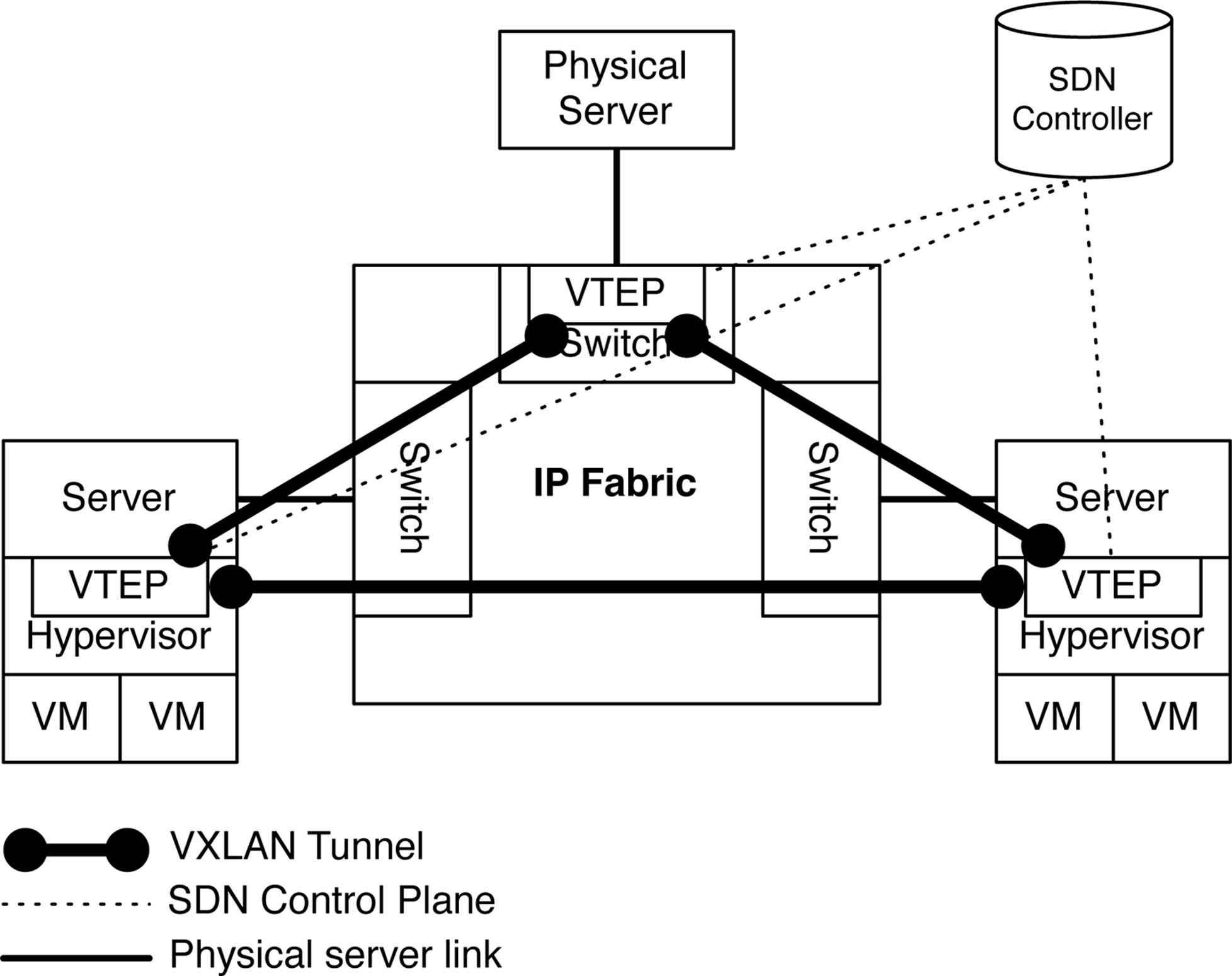
Figure 7-1. Virtual-to-physical data flow in an overlay architecture

Each server on the left and right of the IP Fabric in Figure 7-1 has been virtualized with a hypervisor. Each hypervisor has a VTEP within it that handles the encapsulation of data plane traffic between VMs. Each VTEP also handles MAC address learning, provisioning of new virtual networks, and other configuration changes. The server on top of the IP Fabric is a simple physical server, but doesn’t have any VTEP capabilities of its own. For the physical server to participate in the overlay architecture, it needs something to encapsulate the data plane traffic and perform MAC address learning. Being able to handle the VTEP role within an access switch simplifies the overlay architecture. Now, each access switch that has physical servers connected to it can simply perform the overlay encapsulation and control plane on behalf of the physical server. From the point of view of the physical server, it simply sends traffic into the network without having to worry about anything else.

IP Fabric

To summarize, there are two primary drivers for an IP Fabric: OTT companies with simple Layer 3 requirements, and the introduction of overlay networking that uses the IP Fabric as a foundational underlay. Let’s begin to explore these by taking a look at the requirements of overlay networking in the data center and how an IP Fabric can meet and exceed the requirements.

All VM and server MAC addresses, traffic, and flooding are encapsulated between VTEPs in an overlay architecture. The only network requirements of VTEPs is Layer 3 connectivity. Creating a network that’s able to meet the networking requirements is straightforward. The challenge is in how you design a transport architecture that’s able to scale in a linear fashion as the size increases. A very similar problem was solved back in 1953, by the telecommunications industry. Charles Clos invented a method to create a multistage network that is able to grow beyond the largest switch in the network. This is illustrated in Figure 7-2.

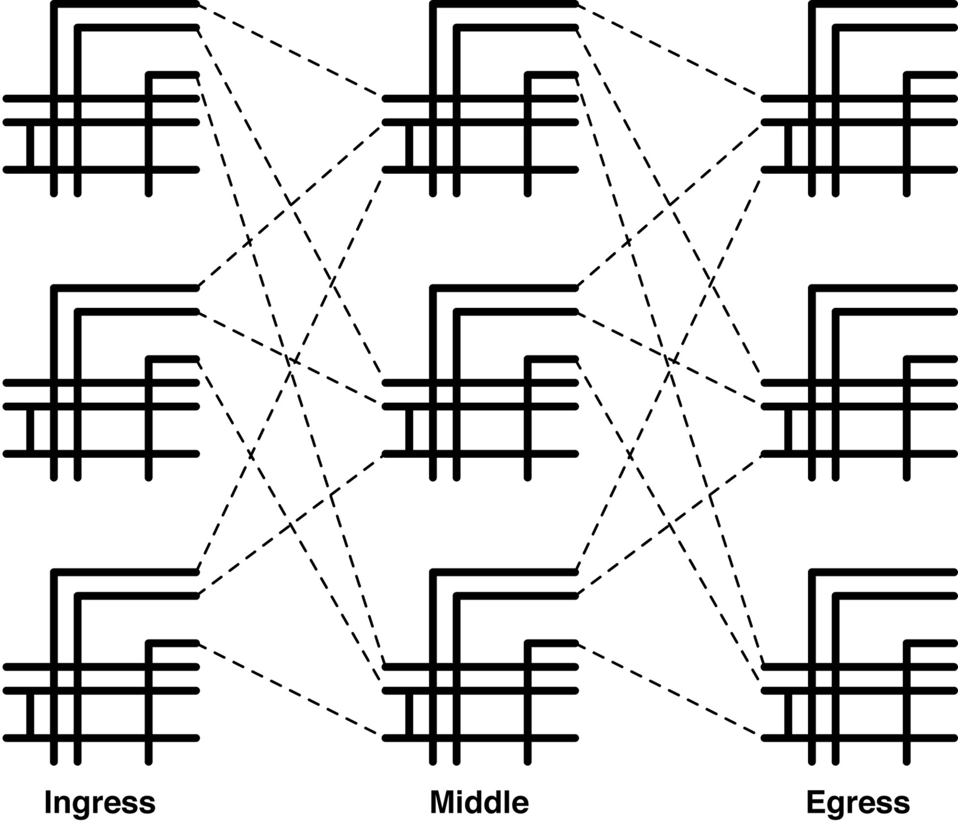
Figure 7-2. Charles Clos’ multistage topology

The advantage to a Clos topology is that it’s nonblocking and provides predictable performance and scaling characteristics. Figure 7-2 represents a 3-stage Clos network: ingress, middle, and egress.

We can take the same principals of the Clos network and apply it to creating an IP Fabric. Many networks are already designed like this and are often referred to as spine-and-leaf networks, which you can see demonstrated in Figure 7-3.

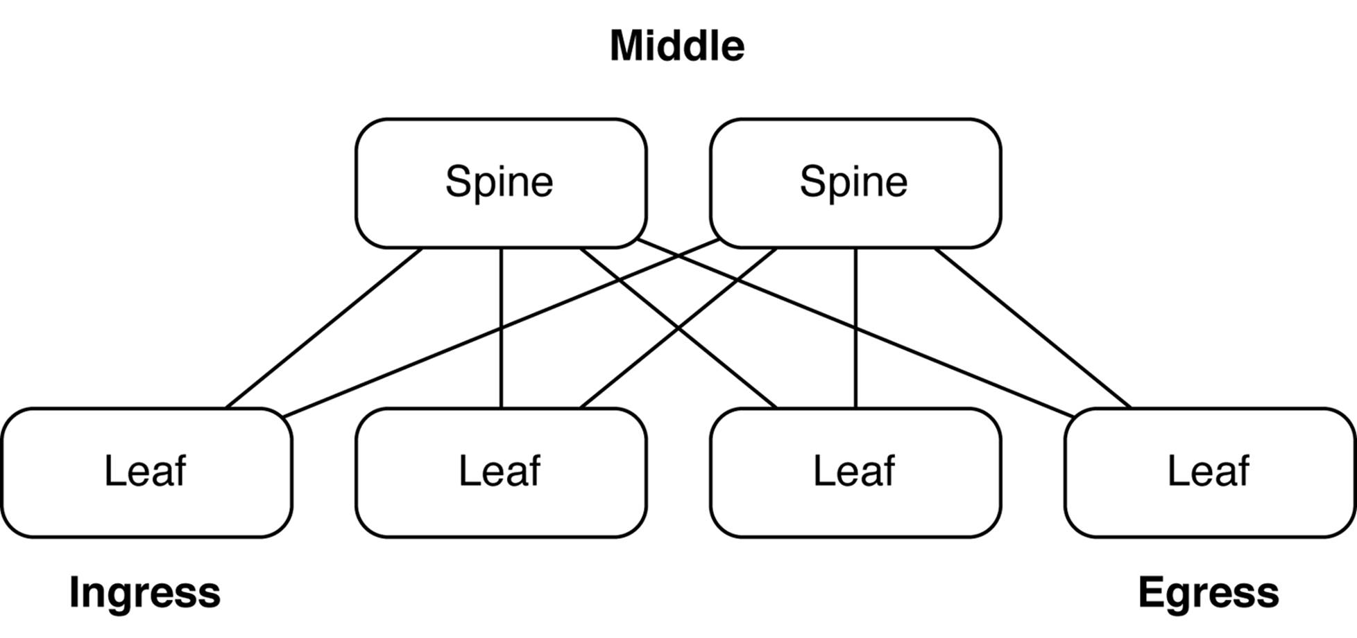
Figure 7-3. Spine-and-leaf topology

A spine-and-leaf network is actually identical to a three-stage Clos network; it is sometimes referred to as a folded three-stage Clos network because the ingress and egress points are folded back on top of each other, as illustrated in Figure 7-3. In this example the spine switches are simple Layer 3 switches and the leaves are top-of-rack (ToR) switches that provide connectivity to the servers and VTEPs.

The secret to scaling up the number of ports in a Clos network is adjusting two values: the width of the spine, and over-subscription ratio. The wider the spine, the more leaves the IP Fabric can support. The more over-subscription placed into the leaves, the larger the IP Fabric, as well. Let’s review some example topologies in detail to understand how the pieces are put together and what the end results are.

768×10GbE Virtual Chassis Fabric

The first example is a new Juniper technology called Virtual Chassis Fabric (VCF) that enables you to create a three-stage IP Fabric by using a set of Juniper QFX5100 switches that are managed as a single device. As of Junos 13.2, the maximum number of switches in a VCF is 20, as depicted in Figure 7-4.

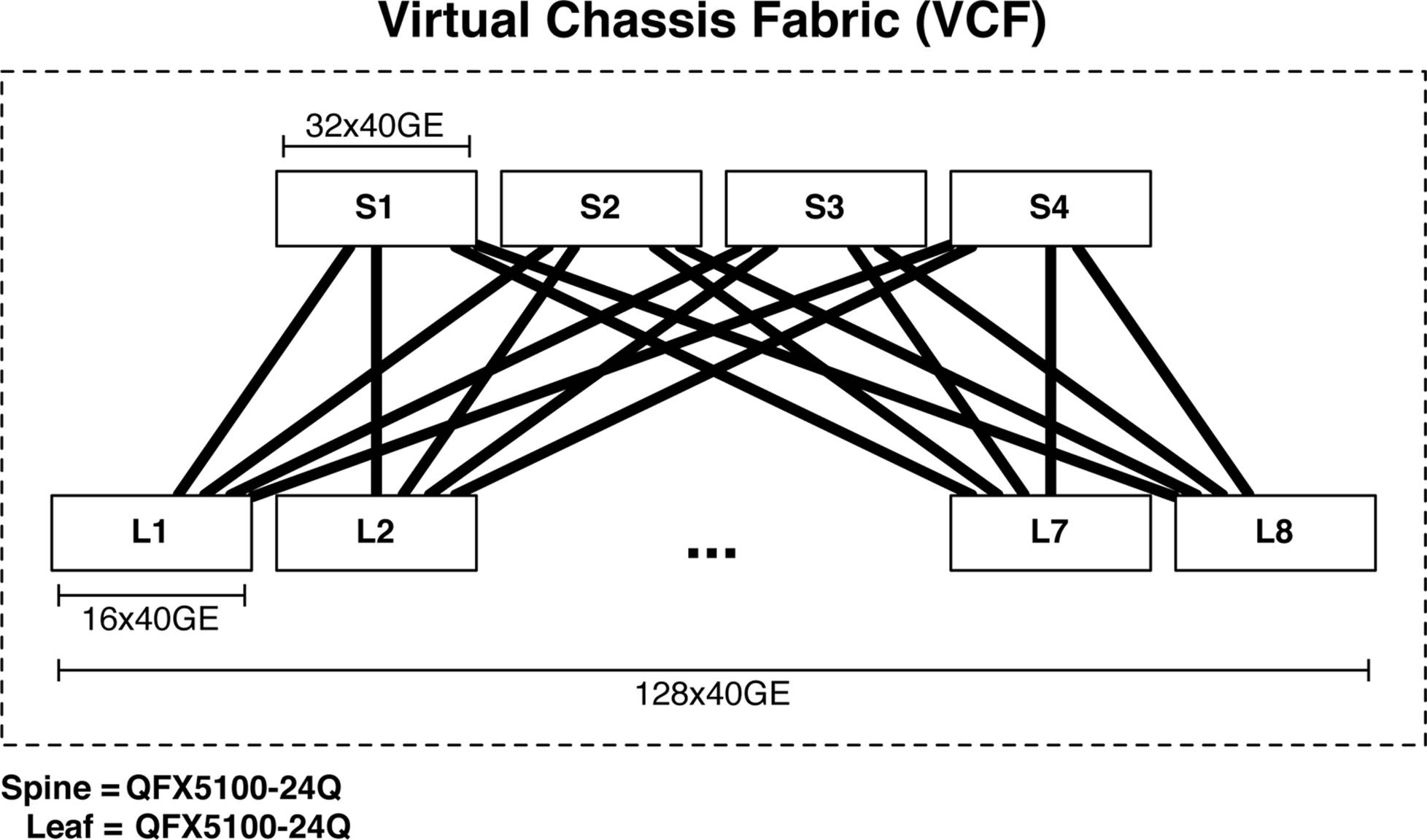
Figure 7-4. VCF of 768 10GbE ports

In this example, the spine comprises four QFX5100-24Q switches; each switch supports up to 32 40GbE interfaces. The leaves are built by using the Juniper QFX5100-48S, which supports 48 10GbE and 6 40GbE interfaces. Each leaf uses 4 40GbE interfaces as uplinks, with one link going to each spine (see Figure 7-4); this creates an over-subscription of 480:160, or 3:1 per leaf. Because VCF only supports 20 switches, we have a total of four spine switches and 16 leaf switches for a total of 20. Each leaf supports 48 10GbE interfaces; because there are 16 leaves total, this brings the total port count up to 768 10GbE, with 3:1 over-subscription.

If you have scaling requirements that exceed the capacity of VCF, it’s not a problem. The next option is to create a simple three-stage IP Fabric that is able to scale to thousands of ports.

3,072×10GbE IP Fabric

The next option is creating a simple three-stage IP Fabric by using the Juniper QFX5100-24Q and QFX5100-96S, but this time we won’t use VCF. The Juniper QFX5100-24Q switch has 32 40GbE ports, and the Juniper QFX5100-96S boasts 96 10GbE and 8 40GbE ports. Combining the Juniper QFX5100-24Q and the Juniper QFX5100-96S creates an IP Fabric of 3,072 usable 10GbE ports, as shown in Figure 7-5.

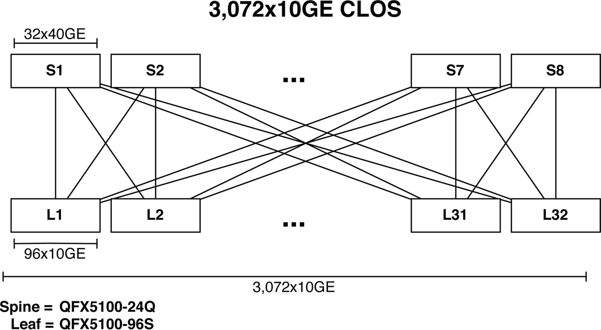
Figure 7-5. 3,072 10GbE IP Fabric topology

The leaves are constructed by using the Juniper QFX5100-96S, and 8 40GbE interfaces are used as uplinks into the spine. Because each leaf has eight uplinks into the spine, the maximum width of the spine is eight. Each 40GbE interface per leaf will connect to a separate spine; thus each leaf will consume one 40GbE interface per spine. To calculate the maximum size of the IP Fabric, you need to multiply the number of server interfaces on the leaf by the number of leaves supported by the spine. In this example, the spine can support 32 leaves, and each leaf can support 96 ports of 10GbE; this is a total of 3,072 usable 10GbE ports with a 3:1 over-subscription ratio.

Control Plane Options

One of the big benefits to using VCF is that you need not worry about the underlying control plane protocols of the IP Fabric. It just works. However, if you need to create a network that exceeds the scale of VCF, you need to take a look at what the control plane options are.

One of the fundamental requirements in creating an IP Fabric is the distribution of prefixes. Each leaf will need to send and receive IP routing information to and from all of the other leaves in the IP Fabric. The question now becomes what are the options for an IP Fabric control plane, and which is the best? We can begin by reviewing the fundamental requirements of an IP Fabric and mapping the results to the control plane options, as is done in Table 7-1.

The most common options for the control plane of an IP Fabric are Open Shortest Path First (OSPF), Intermediate System to Intermediate System (IS-IS), and Border Gateway Protocol (BGP). Each protocol can fundamentally advertise prefixes, but vary in terms of scale and features. OSPF and IS-IS use a flooding technique to send updates and other routing information. Creating areas can help scope the amount of flooding, but then you start to lose the benefits of a Shortest Path First (SPF) routing protocol. On the other hand, BGP was created from the ground up to support a large number of prefixes and peering points. The best use case in the world to prove this point is the Internet.

Having the ability to shift traffic around in an IP Fabric could be useful; for example, you could steer traffic around a specific spine switch while it’s in maintenance. OSPF and IS-IS have limited traffic-engineering and traffic-tagging capabilities. Again, BGP was designed from the ground up to support extensive traffic engineering and tagging with features such as Local Preference, Media Endpoint Discoveries (MEDs), and extended communities.

One of the interesting side effects of building a large IP Fabric is that it’s generally done iteratively and over time. It is common to see multiple vendors creating a single IP Fabric. Although OSPF and IS-IS work well across multiple vendors, the real winner here is BGP. Again, the best use case in the world is the Internet. It consists of a huge number of vendors, equipment, and other variables, but they all use BGP as the control plane protocol to advertise prefixes, perform traffic engineering, and tag traffic.

Because of the scale, traffic tagging, and multivendor stability, BGP is the best choice when selecting a control plane protocol for an IP Fabric. The next question is how do you design BGP in an IP Fabric?

BGP Design

One of the first decisions to make is to whether to use iBGP or eBGP. The very nature of an IP Fabric is based on Equal-Cost Multipath (ECMP). One of the design considerations is how does each option handle ECMP? By default eBGP supports ECMP without a problem. However, iBGP requires a BGP route reflector and the AddPath feature to fully support ECMP.

Let’s take a closer look at the eBGP design in an IP Fabric. Each switch represents a different autonomous system (AS) number and each leaf must peer with every other spine in the IP Fabric, as illustrated in Figure 7-6.

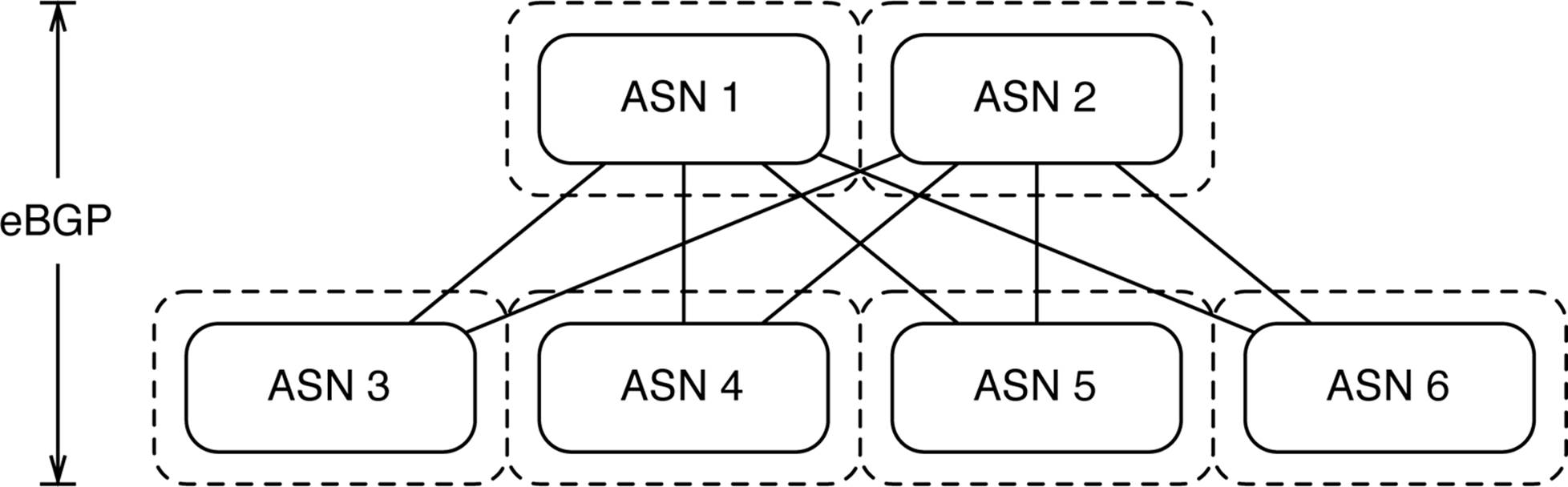
Figure 7-6. Using eBGP in an IP Fabric

Using eBGP in an IP Fabric is very simple and straightforward; it also lends itself well to traffic engineering using Local Preference and AS padding techniques.

Designing iBGP in an IP Fabric is a bit different, due to the requirements of iBGP to have all switches peer with every other device within the IP Fabric. To mitigate the burden of having to peer with every other device in the IP Fabric, we can use inline BGP route reflectors in the spine of the network (see Figure 7-7). The problem with standard BGP route reflection is that it only reflects the best prefix and doesn’t lend itself well to ECMP. To enable full ECMP we must use the BGP AddPath feature, which adds additional ECMP paths into the BGP advertisements between the route reflector and clients.

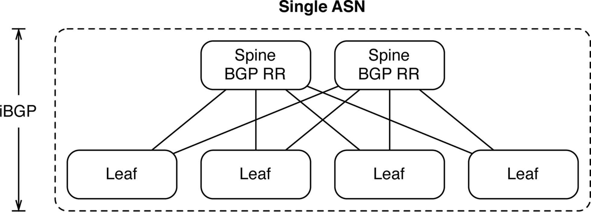
Figure 7-7. Using iBGP in an IP Fabric

The Juniper QFX5100 series supports both the iBGP and eBGP design options. Both options work equally well; however, the design and implementation of eBGP is simpler. Going back to designing a machine with less moving parts is always more stable; it’s our recommendation to use eBGP when creating simple three-stage IP Fabrics. There’s no need to worry about BGP route reflection and AddPath if you’re not required to do so.

Implementation Requirements

There is a set of requirements that need to be worked out in order to create a blueprint for an IP Fabric. At a high level, it revolves around IP Address Management (IPAM) and BGP assignments. The list that follows breaks out the requirements into the next level of detail:

Base IP Prefix

All of the IP address assignments made within the IP Fabric must originate from a common base IP prefix. It’s critical that the base IP prefix have enough address space to hold all of the point-to-point addressing as well as loopback addressing of each switch in the IP Fabric.

Point-to-Point Network Mask

Each leaf is connected to every spine in the IP Fabric; these connections are referred to as the point-to-point links. The network mask used in the point-to-point links will determine how much of the base IP prefix is used. For example, using a 30-bit network mask will use twice as much space as using a 31-bit network mask.

Point-to-Point IP Addresses

For every point-to-point connection, each switch must have an IP address assignment. You need to decide whether the spine receives the lower or higher numbered IP address assignment. This is more of a cosmetic decision and doesn’t impact the functionality of the IP Fabric.

Server-Facing IP Prefix

To provide Layer 3 gateway services to VTEPs, the leaves must have a consistent IP prefix that’s used for server-facing traffic. This is separate from the base IP prefix used to construct the IP Fabric. The server-facing IP prefix must be large enough to support the address requirements of each leaf in the IP Fabric. For example, if each leaf required a 24-bit subnet and there were 512 leaves, the minimum server-facing IP prefix would need to be at least 15 bits, such as 192.168.0.0/15, which would allow you to have 512 24-bit subnets. Each leaf would have a 24-bit subnet such as 192.168.0.0/24 and could use the first IP address for Layer 2 gateway services such as 192.168.0.1/24.

Loopback Addressing

Each switch in the IP Fabric needs a single loopback address using a 32-bit mask. You can use the loopback address for troubleshooting and to verify connectivity between switches.

BGP Autonomous System Numbers

Each switch in the IP Fabric would require its own Autonomous System Numbers (ASN). Each spine and each leaf would have a unique BGP ASN. This would make it possible for eBGP to be used between the leaves and spines.

BGP Export Policy

Each of the leaves needs to advertise its local server-facing IP prefix into the IP Fabric so that all other servers know how to reach it. Each leaf would also need to export its loopback address into the IP Fabric, as well.

BGP Import Policy

Because each leaf only cares about server-facing IP prefixes and loopback addressing, all other addressing of point-to-point links can be filtered out.

Equal Cost Multi-Path Routing

Each spine and leaf should have the ability to load balance flows across a set of equal next-hops. For example, if there are four spine switches, each leaf would have a connection to each spine. For every flow egressing a leaf switch, there should exist four equal next-hops: one for each spine. To do this ECMP routing should be enabled.

These requirements can easily build a blueprint for the IP Fabric. Although the network might not be fully built out from day one, it’s good to have a scaled out blueprint of the IP Fabric so that there’s no question on how to scale out the network in the future.

Decision Points

There are a couple of important decision points when designing an IP Fabric. The first decision is whether to use iBGP or eBGP. At first this might seem like a simple choice, but there are some other variables that make the decision a bit more complicated. The second decision point is actually a fallout of the first: should you use 16-bit or 32-bit ASNs? Let’s walk through the decision points one at a time and take a closer look.

The first decision point should take you back to your JNCIE or CCIE days. What are the requirements of iBGP versus eBGP? We all know that iBGP requires a full mesh to propagate prefixes throughout the topology. However, eBGP doesn’t require a full mesh and is more flexible. Obviously, the reason behind this is loop prevention. To prevent loops, iBGP will not propagate prefixes learned from one iBGP peer to another. Each iBGP switch must have a BGP session to the other to fully propagate routes. On the other hand, eBGP will simply propagate all BGP prefixes to all BGP neighbors; the exception is that any prefixes that contain the switch’s own ASN will be dropped.

iBGP design

Let’s focus on an iBGP design that meets all of the implementation requirements of building an IP Fabric. The first challenge is how do you get around the full mesh requirement of iBGP? The answer will be BGP confederations or route reflection. Given that an IP Fabric is a fixed topology, route reflection lends itself nicely. As demonstrated in Figure 7-8, each spine switch can act as a BGP route reflector, whereas each leaf is a BGP route reflector client.

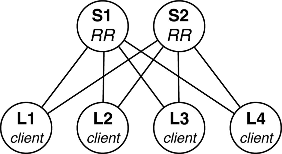
Figure 7-8. iBGP Design with route reflectors

WARNING

It’s important to ensure that the spine switches support BGP route reflection if you want to use an iBGP design. Fortunately, you’re in luck, because the Juniper QFX5100 series supports BGP route reflection.

The other critical implementation requirement that you must meet in an iBGP design is ECMP routing. By default, BGP route reflectors only reflect the best route. This means that if four ECMP routes exist, only the single, best prefix is reflected to the clients. Obviously, this breaks the ECMP requirement and something must be done.

The answer to this problem is to enable the BGP route reflector to send multiple paths instead of the best. There is currently a draft in the IETF that implements this behavior. The feature is called BGP Add Path; with it, the route reflector can offer all ECMP routes to each client.

NOTE

Ensure that the spine switches in your IP Fabric support BGP Add Path if you want to design the network using iBGP. Thankfully, the Juniper QFX5100 family supports BGP Add Path as well as BGP route reflection.

To summarize, the spine switches must support BGP route reflection as well as BGP Add Path to meet all of the IP Fabric requirements with iBGP, but iBGP does allow you to manage the entire IP Fabric as a single ASN.

eBGP Design

The other alternative is to use eBGP to design the IP Fabric. By default, eBGP will meet all of the implementation requirements when building the IP Fabric. There’s no need for BGP route reflection or BGP Add Path with eBGP.

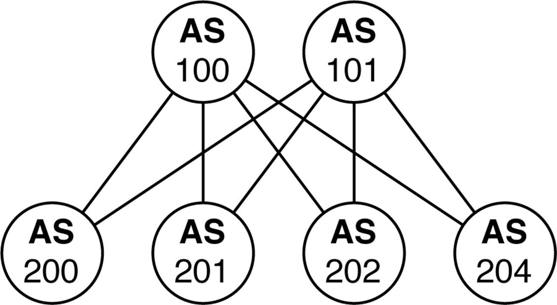
Figure 7-9. eBGP requires a BGP ASN per switch

The only thing you really have to worry about is how many BGP ASNs you will consume with the IP Fabric. Each switch will have its own BGP ASN. Technically the BGP private range is 64,512 to 65,535 (and 65,535 is reserved) which leaves you with 1,023 BGP ASNs. If the IP Fabric is larger than 1,023 switches, you’re going to have to consider moving into the public BGP ASN range or move to 32-bit ASN numbers.

WARNING

As you can see, eBGP has the simplest design that meets all of the implementation requirements. This works well when creating a multivendor IP Fabric.

Edge connectivity

The other critical decision point is how do you connect your data center to the rest of the world and to other data centers? There are multiple decision points due to the number of end points and options. Let’s review a simple example of two data centers. Figure 7-10 gives you an overview.

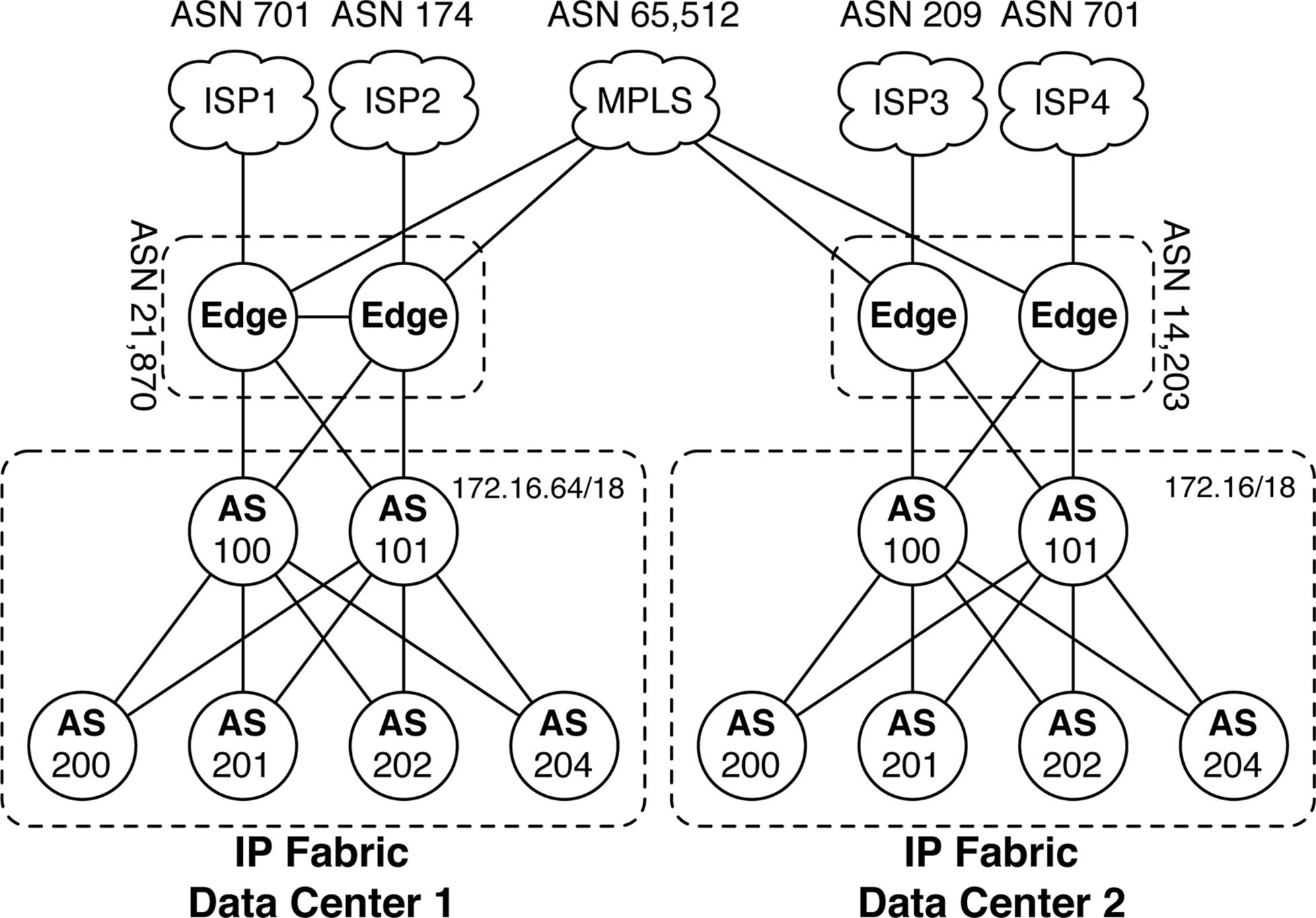
Figure 7-10. Edge connectivity in two data centers with IP Fabrics

Each data center has the following components:

§ An IP Fabric using the same BGP ASN numbers and scheme

§ Two edge routers with a unique BGP ASN

§ They are connected to two ISPs

§ They are connected to a private Multiprotocol Label Switching (MPLS) network

Reusing the same eBGP design in each data center reduces the operational burden of bringing up new data centers; it also creates a consistent operational experience, regardless of which data center you’re in. The drawback is that using the same AS numbers throughout the entire design makes things confusing in the MPLS core. For example, what BGP prefixes does AS 200 own? The answer is that it depends on which data center you’re in.

One simple solution is to use the BGP AS Override feature. This allows the PE routers in the MPLS network to change the AS used by the edge routers in each data center. Now, we can simply say that ASN 21,870 owns the aggregate 172.16.64/18 and ASN 14,203 owns the aggregate 172.16/18. For example, from the perspective of Data Center 1, the route to 172.16/18 is through BGP ASN 65,512 then 14,203. To do this, you must create a BGP export policy on the edge routers in each data center that rejects all of the IP Fabric prefixes but instead advertises a single BGP aggregate.

When connecting out to the Internet, the design is a little different. The goal is that the IP Fabric should have a default route of 0/0, but the edge routers should have a full Internet table. Each data center has its own public IP range that needs to be advertised out to each ISP, as well. In summary, the edge routers will perform the following actions:

§ Advertise a default route into the IP Fabric

§ Advertise public IP ranges to each ISP

§ Reject all other prefixes

IP Fabrics Review

With IP Fabrics, you can create some very large networks that are easily able to support overlay networking architectures in the data center. There are a few decision points that you must consider carefully when creating your own IP Fabric. How many switches will you deploy? Do you want to design for a multivendor environment using BGP features? How many data centers will be connected to each other? These are the questions you must ask yourself and consider into the overall design of each data center.

BGP Implementation

Let’s get down to brass tacks. Moving from the design phase to the implementation phase requires physical devices, configurations, and verification. This section walks through the implementation in detail using Junos. In this laboratory we will have two spines and three leaves, as shown inFigure 7-11.

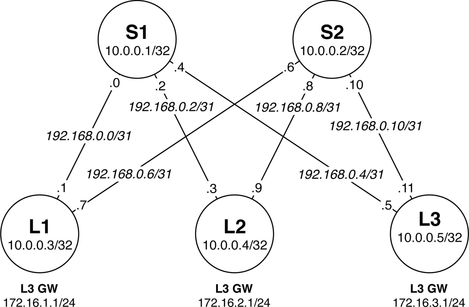
Figure 7-11. BGP implementation of an IP Fabric

There’s a lot happening in Figure 7-11. The following is a breakdown of the IP address schema:

Loopback Address

Each switch will use a 32-bit loopback address from the 10/8 range.

Point-to-Point Addresses

Each switch will use a 31-bit netmask on each point-to-point link starting from 192.168/24.

Layer 3 Server Gateway

Servers connecting to the IP Fabric will require a default gateway. Each leaf will have gateway services starting at 172.16.1/24.

Topology Configuration

The first step is to examine the topology and understand how each switch is connected, what the BGP attributes are, and IP address schemes. Each switch has a hostname, loopback, L3 gateway, and a BGP ASN. Table 7-2 lists the implementation details for you.

NOTE

My apologies for using a public BGP ASN in my lab. Please don’t do this in real life.

Interface and IP Configuration

Now, let’s investigate the physical connection details of each switch. Table 7.3 presents the interface names, point-to-point network, and IP addresses.

Each leaf is connected to each spine, but notice that the spines aren’t connected to one another. In an IP Fabric, there’s no requirement for the spines to be directly connected. Given any single-link failure scenario, all leaves will still have connectivity to one another. The other detail is that an IP Fabric is all Layer 3. Traditional Layer 2 networks require connections between the spines to ensure proper flooding and propagation of the broadcast domains. Yet another reason to favor Layer 3 IP Fabric: no need to interconnect the spines.

BGP Configuration

One of the first steps is to configure each spine to peer via eBGP to each leaf. One trick to speed up the BGP processing in Junos is to keep all the neighbors in a single BGP group. We can certainly do this because the import and export policies are identical, but only the peer AS and neighbor IP vary from leaf to leaf. Here’s the BGP configuration of S1:

protocols {

bgp {

log-updown;

import bgp-clos-in;

export bgp-clos-out;

graceful-restart;

group CLOS {

type external;

mtu-discovery;

bfd-liveness-detection {

minimum-interval 350;

multiplier 3;

session-mode single-hop;

}

multipath multiple-as;

neighbor 192.168.0.1 {

peer-as 200;

}

neighbor 192.168.0.3 {

peer-as 201;

}

neighbor 192.168.0.5 {

peer-as 202;

}

}

}

}

Each leaf has its own neighbor statement with the proper IP address. In addition, each neighbor has its own specific peer AS; this allows all of the leaves in the IP Fabric to be placed under a single BGP group called CLOS.

There are a few global BGP options you’ll want to enable so that you don’t have to specify them for each group and neighbor.

log-updown

This enables tracking of all BGP session state. All groups and neighbors shall inherit this option. Now, we can keep track of the entire IP Fabric from the point of view of each switch.

Import and Export Policies

A common import and export policy is used across the entire IP Fabric; it doesn’t make a difference if it’s a leaf or a spine. We’ll review the policy statements in more detail later in the chapter.

graceful-restart

Of course, you want the ability to make policy changes to BGP without having to tear down existing sessions. To enable this functionality, you can enable the graceful-restart feature in Junos.

Under the CLOS BGP group, we also enable some high-level features:

type external

This enables eBGP for the entire BGP group. Given that the IP Fabric is based on an eBGP design, there’s no need to repeat this information for each neighbor.

mtu-discovery

We’re running jumbo frames on the physical interfaces. Allowing BGP to discover the larger MTU will help in processing control plane updates.

BFD

To ensure that you have fast convergence, you’ll offload the forwarding detection to BFD. In this example, we’re using a 350 ms interval with a 3x multiplier.

multipath multiple-as

To allow for ECMP across a set of eBGP neighbors, you need to enable the multipath multiple-as option.

BGP Policy Configuration

The real trick is writing the BGP policy for importing and exporting the prefixes throughout the IP Fabric. It’s actually straightforward. We can craft a common set of BGP policies to be used across both spines and leaves, which results in a simple copy-and-paste operation.

First up is the BGP export policy:

policy-options {

policy-statement bgp-clos-out {

term loopback {

from {

protocol direct;

route-filter 10.0.0.0/24 orlonger;

}

then {

next-hop self;

accept;

}

}

term server-L3-gw {

from {

protocol direct;

route-filter 172.16.0.0/12 orlonger;

}

then {

next-hop self;

accept;

}

}

}

}

There’s a lot happening in this policy.

term loopback

The first order of business is to identify the switch’s loopback address and export it to all other BGP peers. You can do this by looking at the directly connected interfaces that match 10/24 or longer bitmask; this will quickly identify all loopback addresses across the entire IP Fabric. Personally, I keep next-hop self in the policy just in case there’s a change to iBGP in the future; this way prefixes are still exchanged and next-hops are valid.

term server-L3-gw

We already know that each leaf has Layer 3 gateway services for the servers connected to it; the range is 172.16/12. This will match all of the server gateway addresses on each leaf. Of course, you’ll apply the next-hop self, as well. Obviously, this has no effect on the spines and will only work on the leaves; it’s great being able to write a single policy for both switches.

Default

Each BGP policy has a default term at the very end. It isn’t configurable, but follows the default rules of eBGP: advertise all eBGP and iBGP prefixes to the neighbor; otherwise, deny all other prefixes. This simply means that other BGP prefixes in the routing table will be advertised to other peers. You can stop this behavior by installing an explicit reject action at the end, but in this case you want the IP Fabric to propagate all BGP prefixes to all leaves.

Here’s the import policy configuration:

policy-options {

policy-statement bgp-clos-in {

term loopbacks {

from {

route-filter 10.0.0.0/24 orlonger;

}

then accept;

}

term server-L3-gw {

from {

route-filter 172.16.0.0/12 orlonger;

}

then accept;

}

term reject {

then reject;

}

}

}

Again, there is a lot happening in the import policy. At a high level, you want to be very selective about what types of prefixes you accept into the routing and forwarding table of each switch. Let’s walk through each term in detail.

term loopbacks

Obviously, you want each switch to have reachability to every other switch in the IP Fabric via loopback addresses. You will explicitly match on the 10/8 and allow all loopback addresses into the routing and forwarding table.

term server-L3-gw

The same goes for server Layer 3 gateway addresses; each leaf in the IP Fabric needs to know about all other gateway addresses. You’ll explicitly match on 172.16/12 to allow this.

term reject

At this point, you’ve had enough. Reject all other prefixes. The problem is that if you didn’t have a reject statement at the end of the import policy, the routing and forwarding tables would be trashed by all of the point-to-point networks. There’s no reason to have this information in each switch, because it’s only relevant to the immediate neighbor of its respective switch.

You simply export and import loopbacks and Layer 3 server gateways and propagate all prefixes throughout the entire IP Fabric. The best part is that you can reuse the same set of policies throughout the entire IP Fabric, as well. Copy and paste.

ECMP Configuration

Recall that we used the multipath multiple-as configuration knob in the BGP section. That alone only installs ECMP prefixes into the Routing Information Base (RIB). To take full ECMP from the RIB and install it into the Forwarding Information Base (FIB), you need to create another policy that enables ECMP and install it into the FIB. Here’s the policy:

routing-options {

forwarding-table {

export PFE-LB;

}

}

policy-options {

policy-statement PFE-LB {

then {

load-balance per-packet;

}

}

}

The PFE-LB policy simply says that for any packet being forwarded by the switch, enable load balancing; this enables full ECMP in the FIB. However, the existence of the PFE-LB policy by itself is useless; it must be applied into the FIB directly. This is done under routing-options forwarding-table by referencing the PFE-LB policy.

BGP Verification

Now that you have configured the IP Fabric, the next step is to ensure that the control plane and data plane are functional. We can verify the IP Fabric through the use of show commands to check the state of the BGP sessions, what prefixes are being exchanged, and passing packets through the network.

BGP State

Let’s kick things off by logging into S1 and checking the BGP sessions:

dhanks@S1> show bgp summary

Groups: 1 Peers: 3 Down peers: 0

Table Tot Paths Act Paths Suppressed History Damp State Pending

inet.0

6 6 0 0 0 0

Peer AS InPkt OutPkt OutQ Flaps Last Up/Dwn

State|#Active/Received/Accepted/Damped...

192.168.0.1 200 12380 12334 0 3 3d 21:11:35

2/2/2/0 0/0/0/0

192.168.0.3 201 12383 12333 0 2 3d 21:11:35

2/2/2/0 0/0/0/0

192.168.0.5 202 12379 12333 0 2 3d 21:11:35

2/2/2/0 0/0/0/0

All is well, and each BGP session to each leaf is connected and exchanging prefixes. You can see that each session has two active, received, and accepted prefixes; these are the loopback and Layer 3 gateway addresses. So far, everything is great.

Let’s dig further down the rabbit hole. You need to verify, from a control plane perspective, ECMP, graceful restart, and BFD. Here it is:

dhanks@S1> show bgp neighbor 192.168.0.1

Peer: 192.168.0.1+60120 AS 200 Local: 192.168.0.0+179 AS 100

Type: External State: Established Flags: <Sync>

Last State: OpenConfirm Last Event: RecvKeepAlive

Last Error: Cease

Export: [ bgp-clos-out ] Import: [ bgp-clos-in ]

Options: <Preference LogUpDown PeerAS Multipath Refresh>

Options: <MtuDiscovery MultipathAs BfdEnabled>

Holdtime: 90 Preference: 170

Number of flaps: 3

Last flap event: Stop

Error: 'Cease' Sent: 1 Recv: 1

Peer ID: 10.0.0.3 Local ID: 10.0.0.1 Active Holdtime: 90

Keepalive Interval: 30 Group index: 1 Peer index: 0

BFD: enabled, up

Local Interface: xe-0/0/14.0

NLRI for restart configured on peer: inet-unicast

NLRI advertised by peer: inet-unicast

NLRI for this session: inet-unicast

Peer supports Refresh capability (2)

Stale routes from peer are kept for: 300

Peer does not support Restarter functionality

NLRI that restart is negotiated for: inet-unicast

NLRI of received end-of-rib markers: inet-unicast

NLRI of all end-of-rib markers sent: inet-unicast

Peer supports 4 byte AS extension (peer-as 200)

Peer does not support Addpath

Table inet.0 Bit: 10000

RIB State: BGP restart is complete

Send state: in sync

Active prefixes: 2

Received prefixes: 2

Accepted prefixes: 2

Suppressed due to damping: 0

Advertised prefixes: 3

Last traffic (seconds): Received 1 Sent 25 Checked 42

Input messages: Total 12381Updates 3Refreshes 0Octets 235340

Output messages: Total 12334Updates 7Refreshes 0Octets 234634

Output Queue[0]: 0

The important bits are italicized. Take a closer look at the two lines of Options. You can see the following:

§ Logging the state of the BGP session

§ Support ECMP

§ Support graceful restart

§ MTU discovery enabled

§ BFD is bound to BGP

BGP Prefixes

With BGP itself configured correctly, let’s examine what it’s doing. Take a closer look at S1 and see what prefixes are being advertised to L1:

dhanks@S1> show route advertising-protocol bgp 192.168.0.1 extensive

inet.0: 53 destinations, 53 routes (52 active, 0 holddown, 1 hidden)

* 10.0.0.1/32 (1 entry, 1 announced)

BGP group CLOS type External

Nexthop: Self

Flags: Nexthop Change

AS path: [100] I

* 10.0.0.4/32 (1 entry, 1 announced)

BGP group CLOS type External

Nexthop: Self (rib-out 192.168.0.3)

AS path: [100] 201 I

* 10.0.0.5/32 (1 entry, 1 announced)

BGP group CLOS type External

Nexthop: Self (rib-out 192.168.0.5)

AS path: [100] 202 I

* 172.16.2.0/24 (1 entry, 1 announced)

BGP group CLOS type External

Nexthop: Self (rib-out 192.168.0.3)

AS path: [100] 201 I

* 172.16.3.0/24 (1 entry, 1 announced)

BGP group CLOS type External

Nexthop: Self (rib-out 192.168.0.5)

AS path: [100] 202 I

Things are really looking great. S1 is advertising five prefixes to L1. Here’s a breakdown:

10.0.0.1/32

This is the loopback address on S1 itself. You’re advertising this prefix to L1.

10.0.0.4/32

This is the loopback address for L2. You’re simply passing this prefix on to L1. You can see the AS path is [100] 201 I, which means that the route origin was internal and you can simply follow the AS itself back to L2.

10.0.0.5/32

Same goes for the loopback address of L3. Passing it on to L1.

172.16.2.0/24

This is the Layer 3 gateway address for L2. Passing it on to L1.

172.16.3.0/24

Same goes for the Layer 3 gateway address for L3. Passing it on to L1.

Here’s what you’re receiving from the other leaves:

dhanks@S1> show route receive-protocol bgp 192.168.0.1

inet.0: 53 destinations, 53 routes (52 active, 0 holddown, 1 hidden)

Prefix Nexthop MED Lclpref AS path

* 10.0.0.3/32 192.168.0.1 200 I

* 172.16.1.0/24 192.168.0.1 200 I

dhanks@S1> show route receive-protocol bgp 192.168.0.3

inet.0: 53 destinations, 53 routes (52 active, 0 holddown, 1 hidden)

Prefix Nexthop MED Lclpref AS path

* 10.0.0.4/32 192.168.0.3 201 I

* 172.16.2.0/24 192.168.0.3 201 I

dhanks@S1> show route receive-protocol bgp 192.168.0.5

inet.0: 53 destinations, 53 routes (52 active, 0 holddown, 1 hidden)

Prefix Nexthop MED Lclpref AS path

* 10.0.0.5/32 192.168.0.5 202 I

* 172.16.3.0/24 192.168.0.5 202 I

Again, you can confirm that each leaf is only advertising its loopback and Layer 3 gateway address into the spine.

Routing Table

You have verified that the prefixes are being exchanged correctly between the switches, At this juncture, it’s time to ensure that the RIB is being populated correctly. The easiest way to verify this is to log in to L1 and verify that we see ECMP to the loopback address of L3:

dhanks@L1> show route 172.16.3.1/24 exact

inet.0: 54 destinations, 58 routes (53 active, 0 holddown, 1 hidden)

+ = Active Route, - = Last Active, * = Both

172.16.3.0/24 *[BGP/170] 3d 10:55:14, localpref 100, from 192.168.0.6

AS path: 101 202 I

> to 192.168.0.0 via xe-0/0/14.0

to 192.168.0.6 via xe-0/0/15.0

[BGP/170] 3d 10:55:14, localpref 100

AS path: 100 202 I

> to 192.168.0.0 via xe-0/0/14.0

What we see here is that there are two next-hops to L3 from L1. This is a result of a proper BGP configuration using the multipath multiple-as knob.

Forwarding Table

The next step is to ensure that the forwarding table is being programmed correctly by the RIB. You verify this the same way. Start on L1 and verify to L3:

dhanks@L1> show route forwarding-table destination 172.16.3.1

Routing table: default.inet

Internet:

Destination Type RtRef Next hop Type Index NhRef Netif

172.16.3.0/24 user 0 ulst 131070 5

192.168.0.0 ucst 1702 5 xe-0/0/14.0

192.168.0.6 ucst 1691 5 xe-0/0/15.0

Of course, what you see here are two next-hops: one toward S1 (xe-0/0/14), and the other toward S2 (xe-0/0/15).

Ping

A simple way to verify the data plane connectivity is to log in to L1 and source a ping from its Layer 2 gateway address and ping L3; this will force traffic through the spine of the network:

dhanks@L1> ping source 172.16.1.1 172.16.3.1 count 5

PING 172.16.3.1 (172.16.3.1): 56 data bytes

64 bytes from 172.16.3.1: icmp_seq=0 ttl=63 time=3.009 ms

64 bytes from 172.16.3.1: icmp_seq=1 ttl=63 time=2.163 ms

64 bytes from 172.16.3.1: icmp_seq=2 ttl=63 time=2.243 ms

64 bytes from 172.16.3.1: icmp_seq=3 ttl=63 time=2.302 ms

64 bytes from 172.16.3.1: icmp_seq=4 ttl=63 time=1.723 ms

--- 172.16.3.1 ping statistics ---

5 packets transmitted, 5 packets received, 0% packet loss

round-trip min/avg/max/stddev = 1.723/2.288/3.009/0.414 ms

So far, so good. The trick here is to source the ping from the Layer 3 gateway address; that way you know that L3 has a return route for L1.

Traceroute

To get the next level of detail, let’s use traceroute. You can verify that traffic is moving through the spine of the IP Fabric. Try mixing it up a bit by using the loopback addresses, instead:

dhanks@L1> traceroute source 10.0.0.3 10.0.0.5

traceroute to 10.0.0.5 (10.0.0.5) from 10.0.0.3, 30 hops max, 40 byte packets

1 192.168.0.6 (192.168.0.6) 2.031 ms 1.932 ms 192.168.0.0 (192.168.0.0)

2.121 ms

2 10.0.0.5 (10.0.0.5) 2.339 ms 2.342 ms 2.196 ms

What’s interesting here is that we can see the traceroute happened to go through S2 to get to L3. This is just a result of how the traceroute traffic was hashed by the forwarding table of L1.

Configurations

If you would like to build your own IP Fabric and use this laboratory as a foundation, feel free to use the configuration. For the sake of page count, I share just a single spine and leaf switch. Being an astute reader, you can figure out the rest.

S1

Here is the configuration for S1:

interfaces {

xe-0/0/14 {

mtu 9216;

unit 0 {

family inet {

mtu 9000;

address 192.168.0.0/31;

}

}

}

xe-0/0/16 {

mtu 9216;

unit 0 {

family inet {

mtu 9000;

address 192.168.0.2/31;

}

}

}

xe-0/0/18 {

mtu 9216;

unit 0 {

family inet {

mtu 9000;

address 192.168.0.4/31;

}

}

}

lo0 {

unit 0 {

family inet {

address 10.0.0.1/32;

}

}

}

}

routing-options {

router-id 10.0.0.1;

autonomous-system 100;

forwarding-table {

export PFE-LB;

}

}

protocols {

bgp {

log-updown;

import bgp-clos-in;

export bgp-clos-out;

graceful-restart;

group CLOS {

type external;

mtu-discovery;

bfd-liveness-detection {

minimum-interval 350;

multiplier 3;

session-mode single-hop;

}

multipath multiple-as;

neighbor 192.168.0.1 {

peer-as 200;

}

neighbor 192.168.0.3 {

peer-as 201;

}

neighbor 192.168.0.5 {

peer-as 202;

}

}

}

policy-options {

policy-statement PFE-LB {

then {

load-balance per-packet;

}

}

policy-statement bgp-clos-in {

term loopbacks {

from {

route-filter 10.0.0.0/24 orlonger;

}

then accept;

}

term server-L3-gw {

from {

route-filter 172.16.0.0/12 orlonger;

}

then accept;

}

term reject {

then reject;

}

}

policy-statement bgp-clos-out {

term loopback {

from {

protocol direct;

route-filter 10.0.0.0/24 orlonger;

}

then {

next-hop self;

accept;

}

}

term server-L3-gw {

from {

protocol direct;

route-filter 172.16.0.0/12 orlonger;

}

then {

next-hop self;

accept;

}

}

}

}

L1

And now, the L1 configuration:

interfaces {

interface-range ALL-SERVER {

member-range xe-0/0/0 to xe-0/0/13;

member-range xe-0/0/16 to xe-0/0/47;

unit 0 {

family ethernet-switching {

port-mode access;

vlan {

members SERVER;

}

}

}

}

xe-0/0/14 {

mtu 9216;

unit 0 {

family inet {

mtu 9000;

address 192.168.0.1/31;

}

}

}

xe-0/0/15 {

mtu 9216;

unit 0 {

family inet {

mtu 9000;

address 192.168.0.7/31;

}

}

}

lo0 {

unit 0 {

family inet {

address 10.0.0.3/32;

}

}

}

vlan {

mtu 9216;

unit 1 {

family inet {

mtu 9000;

address 172.16.1.1/24;

}

}

}

}

routing-options {

router-id 10.0.0.3;

autonomous-system 200;

forwarding-table {

export PFE-LB;

}

}

protocols {

bgp {

log-updown;

import bgp-clos-in;

export bgp-clos-out;

graceful-restart;

group CLOS {

type external;

mtu-discovery;

bfd-liveness-detection {

minimum-interval 350;

multiplier 3;

session-mode single-hop;

}

multipath multiple-as;

neighbor 192.168.0.0 {

peer-as 100;

}

neighbor 192.168.0.6 {

peer-as 101;

}

}

}

}

policy-options {

policy-statement PFE-LB {

then {

load-balance per-packet;

}

}

policy-statement bgp-clos-in {

term loopbacks {

from {

route-filter 10.0.0.0/24 orlonger;

}

then accept;

}

term server-L3-gw {

from {

route-filter 172.16.0.0/12 orlonger;

}

then accept;

}

term reject {

then reject;

}

}

policy-statement bgp-clos-out {

term loopback {

from {

protocol direct;

route-filter 10.0.0.0/24 orlonger;

}

then {

next-hop self;

accept;

}

}

term server-L3-gw {

from {

protocol direct;

route-filter 172.16.0.0/12 orlonger;

}

then {

next-hop self;

accept;

}

}

term reject {

then reject;

}

}

}

vlans {

SERVER {

vlan-id 1;

l3-interface vlan.1;

}

}

Summary

This chapter covered the basic ways to build an IP Fabric. More important, it has reviewed the decision points you must take into account when building an IP Fabric. There are various options in the control plane that impact what features are required on the platform. Finally, we reviewed in great detail how to implement BGP in an IP Fabric. We walked through all of the interfaces, IP addresses, BGP configurations, and policies. To wrap things up, we verified that BGP is working across the IP Fabric and ran some tests on the data plane to ensure that traffic can get from leaf to leaf.

Building an IP Fabric is a straightforward task and serves as a great foundation to overlay technologies such as VMware NSX and Juniper Contrail. Basing the design on only Layer 3 makes the IP Fabric very resilient to failure and offers very fast end-to-end convergence with BFD. Build your next IP Fabric with the Juniper QFX5100 series.

Chapter Review Questions

1. How do you avoid full mesh requirements in an iBGP design?

1. BGP route reflection

2. BGP confederations

3. All of the above

4. None of the above

2. What is required to enable ECMP in an iBGP design?

1. Multiple route reflectors

2. Enable load balancing

3. BGP Add Path

4. multipath multiple-as

3. How many private BGP ASNs are there?

1. 1,023

2. 1,024

3. 511

4. 512

Chapter Review Answers

1. Answer: C.

Both are valid options. I recommend using BGP route reflectors. The Juniper QFX5100 family can easily handle both.

2. Answer: C.

You require BGP Add Path for the route reflector to advertise all equal next-hops instead of the best.

3. Answer: A.

There are 1,023 private BGP ASNs.