Juniper QFX5100 Series (2015)

Chapter 9. Network Analytics

One of the most difficult tasks in network operations is gathering accurate sampling data from a switch to create a dashboard that shows the overall health of the network. Accurate network visibility and analytics is the cornerstone to operating an efficient and reliable network. After all, how do you know that your network is running smoothly if you have no idea what’s going across it?

Network analytics is a broad term, but in general—as network operators—we want to provide context and answer the following questions:

§ What types of applications are consuming network resources?

§ What’s the current capacity and utilization of a given switch?

§ How can I quickly identify peaks and valleys?

§ How can I detect microbursts?

§ Are there hotspots forming in the network?

Answering these questions has become more difficult with the standardization of 10GbE access ports in the data center. The amount of traffic is increasing rapidly and traditional sampling techniques such as sFlow and IPFIX only provide answers to some of the questions posed. Because microbursts and latency spikes can happen in very small windows, tools that rely on sampling every few seconds are unable to detect these events that interrupt business applications. Microburst events occur when there are multiple ports of ingress traffic that’s all destined to a single egress port, and the egress port’s buffer is exceeded. For example, if server 1 sent a query to a set of compute clusters, and all 100 compute clusters responded back to the server at the exact same time, the physical port connected to server 1 would become congested for that brief moment in time.

To detect micro events in the network, the frequency at which the networking device samples the traffic and counters must be increased dramatically. With Juniper Enhanced Analytics, you can receive real-time information from the switch and detect events such as latency, jitter, and microbursting.

Overview

The Juniper QFX5100 series gives you the capability to quickly gather traffic statistics and other data out of the switch and into powerful collection tools so that you can visualize what’s happening inside the network (see Figure 9-1). Juniper QFX5100 switches supports two major types of network analytics:

Sampled Data

The sFlow technology on the Juniper QFX5100 family uses sampling to gather data. You can sample interface statistics and flow data on a Juniper QFX5100 switch at a frequency of one out of n packets. Data is exported from the Juniper QFX5100 every 1,500 bytes or every 250 ms. Due to the nature of sampling, there are no options to enable monitoring thresholds; this means you’re unable to send real-time alerts based on events exceeding or dropping below a threshold.

Real-Time Data

Juniper Enhanced Analytics fills in the gaps of traditional sampling techniques such as sFlow. Data is exported from the switch in real time as the data is collected. Enhanced Analytics offers much faster polling intervals, all the way down to 8 ms. Because data is collected in real time, you are able to set high and low thresholds for latency and queue depth, all the way down to 1 nanosecond.

One of the benefits of sFlow is that it’s able to capture the first 128 bytes of the sampled packets. It’s a small form of Deep Packet Inspection (DPI), which remote tools can use to create detailed graphs of the application traffic within the network. Although Enhanced Analytics doesn’t have any (current) DPI capabilities, it has the unique ability to detect micro events and report them in real time. By combining the power of sampled and real-time data, you can get a true end-to-end view of what’s happening within your network.

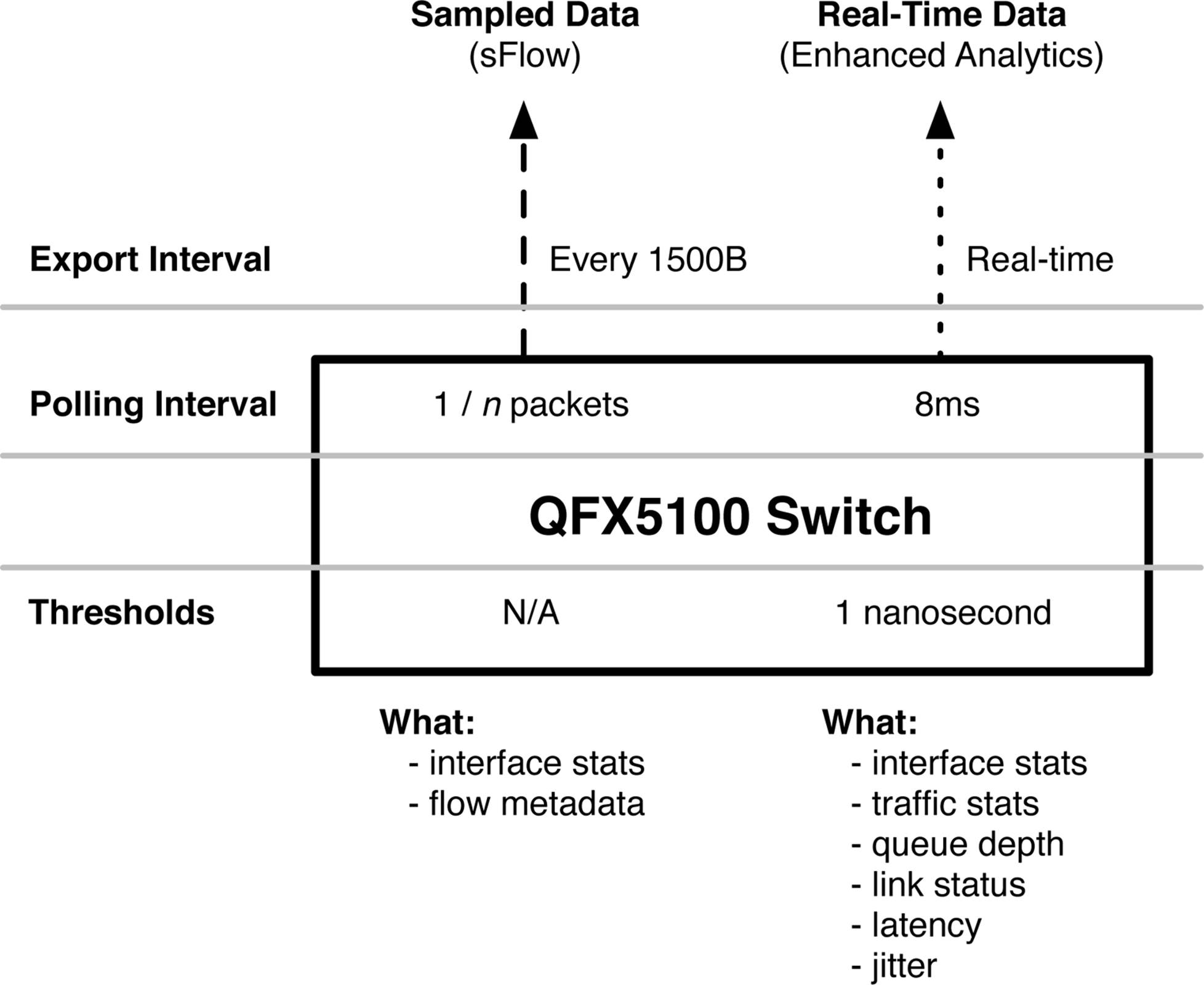
Figure 9-1. Overview of network analytics on the Juniper QFX5100 switch

sFlow

Figure 9-2 shows at a high level how sFlow collects samples of packets in a switched network and sends the aggregated data to a remote collector.

There are two sampling mechanisms for sFlow:

Packet-Based Sampling

You can sample one packet out of a specified number of packets from a particular interface. The first 128 bytes—including the raw Ethernet frame—are recorded and sent to the collector. It’s important to note that only switched traffic can be subject to sFlow; you cannot sample Layer 3 interfaces. The data included in the sampled information is the aforementioned Ethernet frame, IP packet, TCP segments or UDP datagrams, and any remaining payload information up to 128 bytes.

Time-Based Sampling

Using this mode, you can capture interface statistics at a specified time interval to the remote collector. If you don’t need to sample packets and get the first 128 bytes of information but instead only want to receive traffic statistics, time-based sampling would be a good option for you.

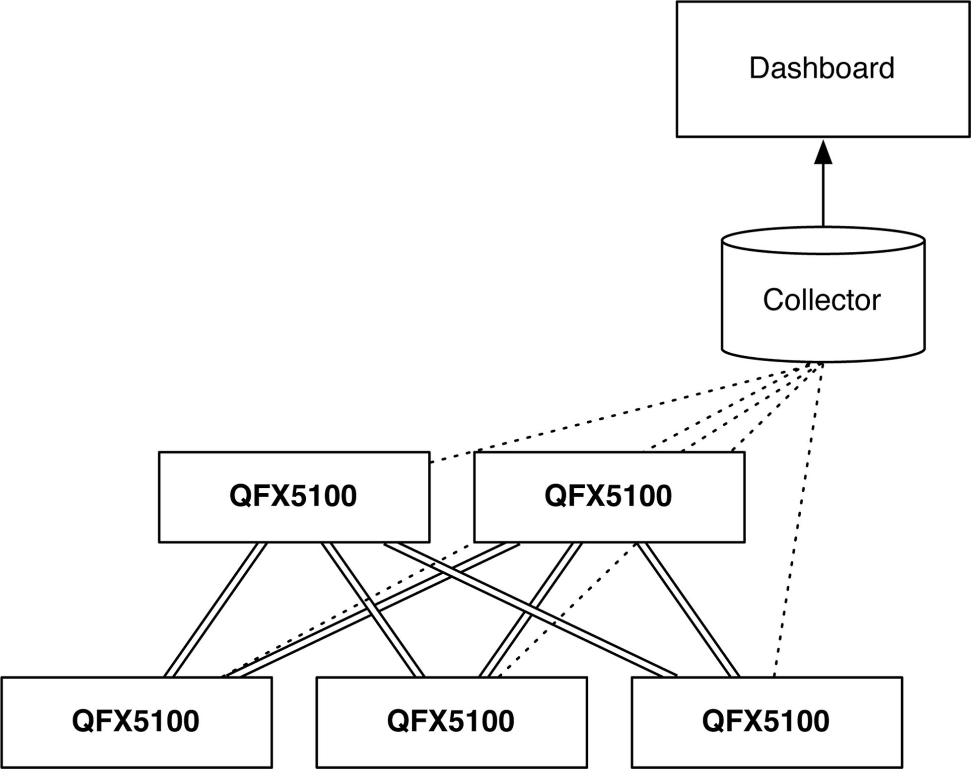
Figure 9-2. Overview of sFlow sampling

sFlow is commonly used to enable network dashboards using collection tools such as PRTG or nfsen. It shows what types of applications are consuming networking resources. Because the first 128 bytes of the packet are sent to the collector, it can easily perform DPI into the payload of the packet and see what’s happening from an application perspective.

Adaptive Sampling

As you might imagine, enabling sFlow across all interfaces in a switch that could support 104 10GbE interfaces would require a lot of processing to sample packets, perform DPI, and send that data to an external collector. You wouldn’t want sFlow to cause any service interruptions to the actual traffic itself. Juniper sFlow includes the capability to monitor the interface traffic and dynamically adjust the polling interval of sFlow.

Agents check the interfaces every 5 seconds and create a sorted list of interfaces that are receiving the most samples per second. The top five interfaces with the highest number of samples are selected. Using a binary backoff algorithm, the sampling loads on the selected interfaces are reduced by half and allocated to other interfaces that have a lower sampling rate. Keep in mind that adaptive sampling is a transient feature that’s adjusted every 5 seconds. If traffic spiked for 1 minute and then went back down for the next 15 minutes, the adaptive sampling would kick in for the first minute, but then restore sFlow to the configured values for the remaining 15 minutes. Sampling resources are distributed evenly across the entire switch during excessive traffic peaks, resulting in the guaranteed delivery of production traffic through the switch.

Configuration

Be aware that an external collection tool is required to make sFlow useful. Downloading and installing an external collection tool is beyond the scope of this book and is left as an exercise to the user. However some of the better sFlow tools are Juniper’s STRM, PRTG, ntop, nfsen, and sFlowTrend.

The first step in the configuration process is to set up the sFlow collector to which we want to send the sampled data. The Juniper QFX5100 series supports sending data from the management port as well as any revenue ports configured for Layer 3. It’s recommended to use revenue ports to export sampled data, because during peak traffic loads, the amount of data being exported can be quite large.

Let’s get right to it:

{master:0}[edit]

dhanks@QFX5100# set protocols sflow collector 192.168.1.100 udp-port 5000

Next, define which interfaces will be enabled for sFlow sampling. By default all the interfaces are excluded from sFlow, and you must enable them for sFlow to work:

{master:0}[edit]

dhanks@QFX5100# set protocols sflow interfaces et-0/0/0

The final step is to set up the polling interval and sampling rate for the interfaces. You can define these settings per interface or simply set them globally:

{master:0}[edit]

dhanks@QFX5100# set protocols sflow sample-rate egress 10 ingress 10

{master:0}[edit]

dhanks@QFX5100# set protocols sflow polling-interval 5

You might be wondering what the difference is between the polling-interval and the sampling-rate; these two knobs are often confused. The polling-interval simply instructs the Juniper QFX5100 device to poll the physical interface every n seconds to collect interface statistics. The sampling-rate specifies how many packets the Juniper QFX5100 switch inspects in order to send sampled meta-information (the first 128 bytes) to the collector.

sFlow Review

The Juniper QFX5100 family of switches supports sFlow for all switched traffic passing through the switch. It allows you to quickly get an idea of what types of applications are consuming networking resources. There are only a few configuration statements to enable sFlow and it’s very easy to get running. However, there are a few caveats, which are listed here:

§ You cannot enable sFlow on Layer 3 interfaces or aggregated Ethernet bundles (ae); however, you can enable sFlow on the member interfaces such as et-0/0/0.

§ When using sFlow on ingress traffic, none of the CPU-bound traffic is captured.

§ When using sFlow on egress traffic, no multicast or broadcast traffic is sampled. Also the Juniper QFX5100 device doesn’t factor in egress firewall filters when using sFlow, due to a limitation in the Broadcom chipset.

§ The Juniper QFX5100 series supports sFlow version 5 as of 13.1X51D20.

Using sFlow is a great way to quickly sample application traffic in your network and visualize it. After enabling sFlow, many network operators are surprised to learn what types of applications and end-user traffic is going across the network.

Enhanced Analytics

With the introduction of 10GbE and higher speeds in the access layer, new use cases have emerged such as Big Data and High-Frequency Trading (HFT). Each of these requires high-speed networks, low latency, and no jitter. Traditional monitoring tools such as sFlow aren’t equipped to deal with the high-speed latency and jitter problems that can arise in high-speed networks. This is because sFlow works by sampling traffic. For example if sFlow only sampled one packet out of 2,000, it wouldn’t be able to detect a microburst happening in the other 1,999 packets.

Overview

With Juniper Enhanced Analytics, you can monitor the Juniper QFX5100 in real time (as opposed to sampling packets) to monitor traffic statistics, queue depth, latency, and jitter in the network (see Figure 9-3). Being able to collect real-time traffic statistics offers more granularity when graphing traffic patterns across interfaces. The queue depth and latency are early warning signals to application failures. For example, if you notice an increasing amount of tail-dropping or microbursts on a specific server, you know that it will have a negative impact on the application performance and reliability.

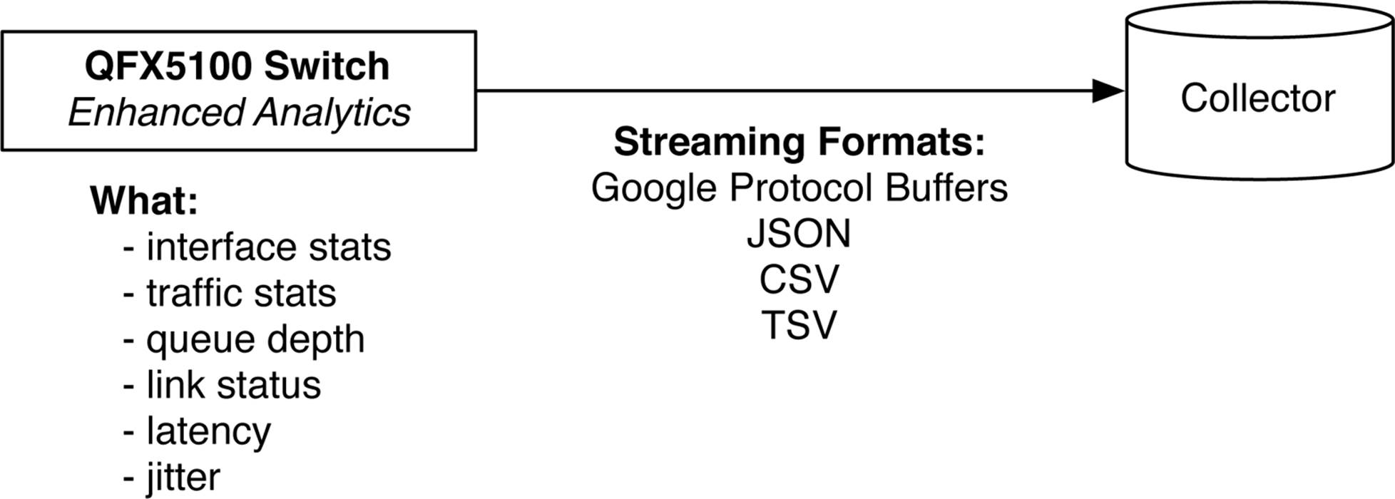
Figure 9-3. Overview of Juniper Enhanced Analytics

Enhanced Analytics is split into two major functions; the result is that a Juniper QFX5100 device is able to quickly export data to multiple collectors in real time for offline analysis. Following is a brief description of each function:

Analytics Daemon

The analytics daemon (analyticsd) runs within Junos; its primary responsibility is to collect the analytics information from the Packet Forwarding Engine (PFE) and export it to the collectors.

Analytics Manager

The analytics manager (AM) runs within the PFE so that it’s able to read traffic, queue depth, and latency in real time. Traffic is read off the data plane and processed into ring buffers so that analyticsd can retrieve the information.

Enhanced Analytics and sFlow make a perfect combination when you need to quickly get all the data off the switch and into offline analysis tools. You get both the benefits of sampled and real-time data to create a true end-to-end view of your network.

Architecture

Both analyticsd (AD) and AM work as a team to obtain real-time data from the PFE and export it to remote collectors, as shown in Figure 9-4.

The two analytics engines, AD and AM, work in unison and use standard Unix Interprocess Communication (IPC) to pass information back and forth. The heavy lifting is performed by the Junos µKernel. Traffic statistics are gathered from the Broadcom chipset every second, and the queue depth information is retrieved every 8 ms (see Figure 9-5). The information is put into ring buffers that the IPC thread uses to retrieve the information; the traffic statistics are pulled from the ring queue every second, and the queue depth is pulled from the ring queue every 100 ms. The rest of the processing is handled by the control plane with the analytics daemon. AD uses standard IPC to transfer data from the AM. From this point the data is shipped off to the configured collectors.

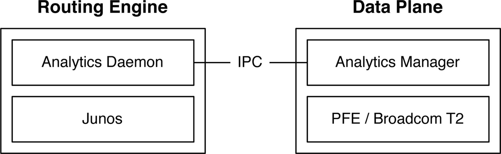
Figure 9-4. Analytics daemon and analytics manager overview

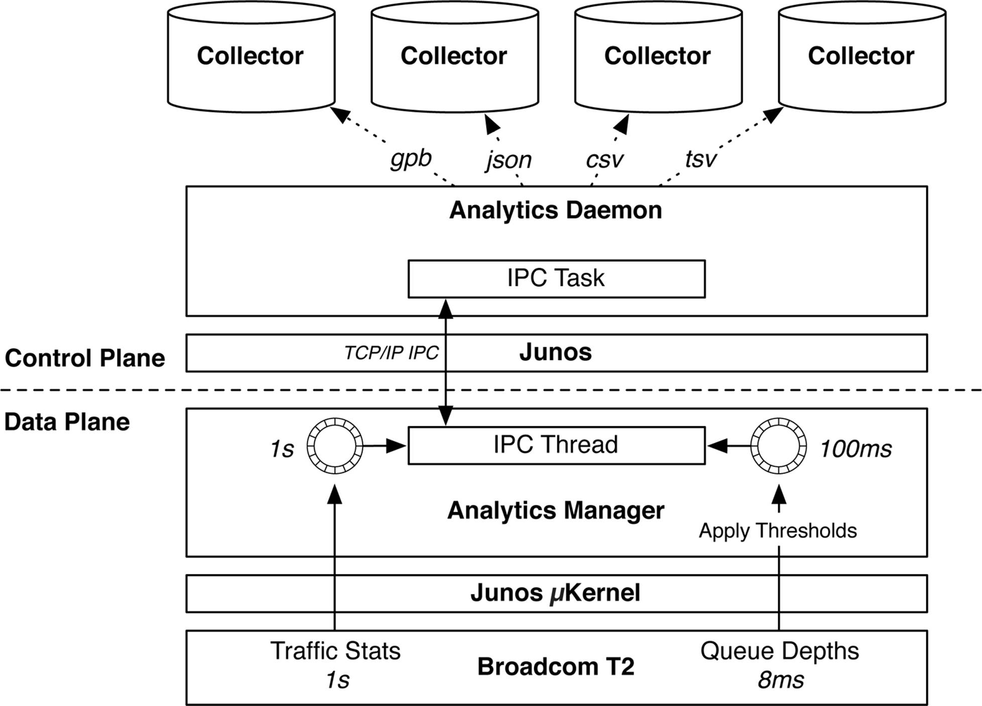
Figure 9-5. Enhanced Analytics architecture

The end result is that data is retrieved from the data plane in real time and exported to multiple collectors. The information gathered makes it possible for you to quickly determine the overall network performance, health, and application stability.

NOTE

The Enhanced Analytics architecture shown in Figure 9-5 is accurate as of Junos 13.1X51D20. Given that the entire architecture is a software solution, it can be changed and enhanced at any time with future software releases.

Streaming Information

The information provided by Enhanced Analytics is critical in mapping out your network to detect latency and jitter between applications. The information streamed is divided into two major categories:

Streamed Queue Depth Statistics

You can use the queue depth information to measure an interface’s latency and see how full the transmit buffer is. If the buffer capacity is exceeded, traffic will drop.

Streamed Traffic Statistics

You can use the traffic statistics to see the amount and velocity of traffic flowing through the network. The information also includes any types of errors and dropped packets.

Using the combination of queue depth and traffic statistics, you can quickly troubleshoot application issues in your data center. The extensive support for streaming protocols reduces the burden to create customized monitoring tools and increases the compatibility with open source tools, such as LogStash, fluentd, and Elasticsearch.

Streaming formats

Enhanced Analytics is capable of streaming the queue depth and traffic information to multiple collectors in the following streaming formats:

Google Protocol Buffer

The Google Protocol Buffer (GPB) supports nine types of messages in a hierarchical format. The format is in binary and isn’t readable by humans, unless you’re Cypher from The Matrix.

JavaScript Object Notation (JSON)

JSON is a lightweight data-interchange format that is easy for both humans and machines to read and parse. It’s based on a subset of the JavaScript Programming Language.

Comma-Separated Values (CSV)

This is a simple flat file containing fields of data delimited by a single comma (“,”).

Tab-Separated Values (TSV)

Simple flat file containing fields of data delimited by a single tab (“\t”).

Each format has its advantages and disadvantages. If you need quick and dirty, you might opt for the CSV or TSV formats. If you really enjoy programming in Python or Perl, you might like to use the JSON format. If you need sheer speed and support for remote procedure calls (RPCs), you might lean toward GPB.

GPB

Take a moment to examine the GPB format, as presented in Table 9-1.

The Juniper QFX5100 family uses a specific GPB prototype file (analytics-proto) to format the streaming data, which you can download from the Juniper website.

Let’s take a look at the fields of the analytics-proto file. This is what you will need to use in your GPB collector:

package analytics;

// Traffic statistics related info

message TrafficStatus {

optional uint32 status = 1;

optional uint32 poll_interval = 2;

}

// Queue statistics related info

message QueueStatus {

optional uint32 status = 1;

optional uint32 poll_interval = 2;

optional uint64 lt_high = 3;

optional uint64 lt_low = 4;

optional uint64 dt_high = 5;

optional uint64 dt_low = 6;

}

message LinkStatus {

optional uint64 speed = 1;

optional uint32 duplex = 2;

optional uint32 mtu = 3;

optional bool state = 4;

optional bool auto_negotiation= 5;

}

message InterfaceInfo {

optional uint32 snmp_index = 1;

optional uint32 index = 2;

optional uint32 slot = 3;

optional uint32 port = 4;

optional uint32 media_type = 5;

optional uint32 capability = 6;

optional uint32 porttype = 7;

}

message InterfaceStatus {

optional LinkStatus link = 1;

optional QueueStatus queue = 2;

optional TrafficStatus traffic = 3;

}

message QueueStats {

optional uint64 timestamp = 1;

optional uint64 queue_depth = 2;

optional uint64 latency = 3;

optional string traffic_class = 4;

}

message TrafficStats {

optional uint64 timestamp = 1;

optional uint64 rxpkt = 2;

optional uint64 rxucpkt = 3;

optional uint64 rxmcpkt = 4;

optional uint64 rxbcpkt = 5;

optional uint64 rxpps = 6;

optional uint64 rxbyte = 7;

optional uint64 rxbps = 8;

optional uint64 rxdrop = 9;

optional uint64 rxerr = 10;

optional uint64 txpkt = 11;

optional uint64 txucpkt = 12;

optional uint64 txmcpkt = 13;

optional uint64 txbcpkt = 14;

optional uint64 txpps = 15;

optional uint64 txbyte = 16;

optional uint64 txbps = 17;

optional uint64 txdrop = 18;

optional uint64 txerr = 19;

}

//Interface message

message Interface {

required string name = 1;

optional bool deleted = 2;

optional InterfaceInfo information = 3;

optional InterfaceStatus status = 4;

optional QueueStats queue_stats = 5;

optional TrafficStats traffic_stats = 6;

}

message SystemInfo {

optional uint64 boot_time = 1;

optional string model_info = 2;

optional string serial_no = 3;

optional uint32 max_ports = 4;

optional string collector = 5;

repeated string interface_list = 6;

}

message SystemStatus {

optional QueueStatus queue = 1;

optional TrafficStatus traffic = 2;

}

//System message

message System {

required string name = 1;

optional bool deleted = 2;

optional SystemInfo information = 3;

optional SystemStatus status = 4;

}

JSON

Following are two examples of JSON. The first example will be queue depth information:

{"record-type":"queue-stats","time":1383453988263,"router-id":"qfx5100-switch",

"port":"xe-0/0/18","latency":0,"queue-depth":208}

The next example is traffic statistics:

{"record-type":"traffic-stats","time":1383453986763,"router-id":"qfx5100-switch",

"port":"xe-0/0/16","rxpkt":26524223621,"rxpps":8399588,"rxbyte":3395100629632,

"rxbps":423997832,"rxdrop":0,"rxerr":0,"txpkt":795746503,"txpps":0,"txbyte":1018555

33467, "txbps":0,"txdrop":0,"txerr":0}

CSV

Now, let’s explore CSV, using the same data as last time. First up is the queue depth information:

q,1383454067604,qfx5100-switch,xe-0/0/18,0,208

Here are the traffic statistics:

t,1383454072924,qfx5100-switch,xe-

0/0/19,1274299748,82950,163110341556,85603312,0,0,

27254178291,8300088,3488534810679,600002408,27268587050,3490379142400

TSV

Finally we have TSV. It’s the exact same thing as CSV, but uses a tab (\t) instead of a comma (“,”) for a delimiter. First up is the queue depth information:

Q 585870192561703872 qfx5100-switch xe-0/0/18 (null) 208 2

You get the idea. There’s no need to show you the traffic statistics.

Streamed queue depth information

The streamed queue depth information is straightforward and makes it possible for you to easily see each interface’s buffer utilization and latency. Table 9-2 lists the data collected in detail.

Streamed traffic information

The streamed traffic information has a very similar format to the queue depth information. Take a look at each of the fields, as shown in Table 9-3.

Configuration

The configuration of Enhanced Analytics is very modular in nature. At a high level, there are resources that reference resource-profiles and there are collectors that reference export-profiles, as shown in Figure 9-6.

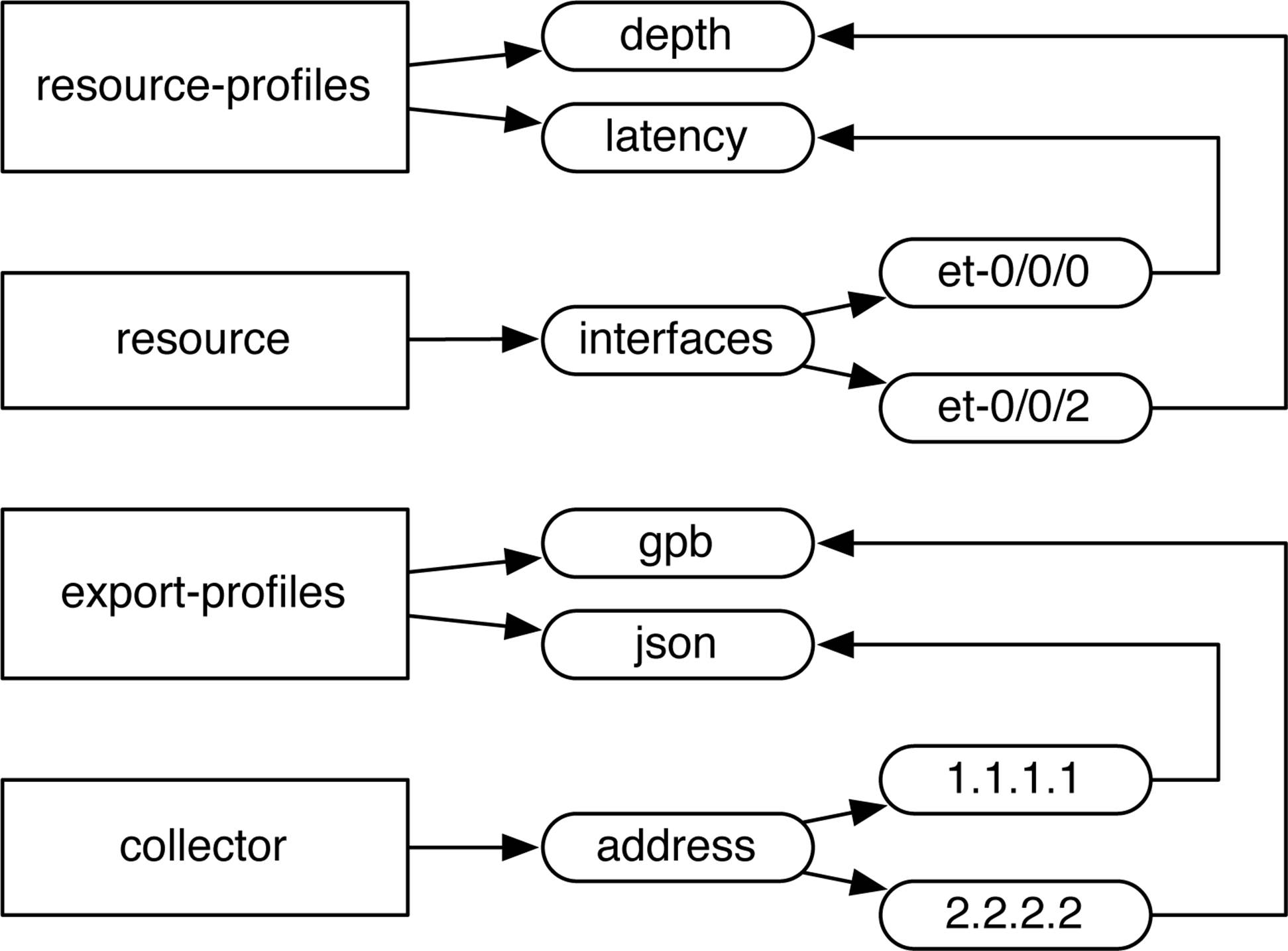
Figure 9-6. Enhanced Analytics configuration hierarchy

Because the configuration is modular in nature, you can create a single Enhanced Analytics configuration that contains multiple profiles for different applications, collectors, and streaming formats. Changing the way a Juniper QFX5100 switch performs analytics is as simple as changing a profile, which triggers all of the underlying changes such as collector addressing, streaming formats, latency thresholds, and traffic statistics.

Let’s inspect the full configuration that’s illustrated in Figure 9-6. We’ll define the following:

§ Two resource profiles

§ Two export profiles

§ Monitor two interfaces

§ Create two collectors with different streaming formats

Here is the code:

services {

analytics {

traceoptions {

file an size 10m files 3;

}

export-profiles {

GPB {

stream-format gpb;

interface {

information;

statistics {

traffic;

queue;

}

status {

link;

traffic;

queue;

}

}

system {

information;

status {

traffic;

queue;

}

}

}

JSON {

stream-format json;

interface {

information;

statistics {

traffic;

queue;

}

status {

link;

traffic;

queue;

}

}

system {

information;

status {

traffic;

queue;

}

}

}

}

resource-profiles {

QUEUE-DEPTH-STANDARD {

queue-monitoring;

traffic-monitoring;

depth-threshold high 14680064 low 1024;

}

LATENCY {

queue-monitoring;

traffic-monitoring;

latency-threshold high 900000 low 100;

}

}

resource {

system {

resource-profile QUEUE-DEPTH-STANDARD;

polling-interval {

traffic-monitoring 2;

queue-monitoring 100;

}

}

interfaces {

et-0/0/0 {

resource-profile QUEUE-DEPTH-STANDARD;

}

et-0/0/1 {

resource-profile LATENCY;

}

}

}

collector {

local {

file an.local size 10m files 3;

}

address 1.1.1.1 {

port 3000 {

transport udp {

export-profile GPB;

}

}

}

address 2.2.2.2 {

port 5555 {

transport tcp {

export-profile JSON;

}

}

}

}

}

}

It’s just like building blocks. You define a set of attributes and then reference it in another part of the configuration. This makes Enhanced Analytics a breeze.

NOTE

There are some tricks that you need to be aware of when configuring the queue depth thresholds. The values are given in bytes, but it’s all relative to the physical interface being monitored.

Here are the calculations for latency, given in bytes for different speed interfaces:

§ 1GbE latency = bytes / 125

§ 10GbE latency = bytes / 1250

§ 40GbE latency = bytes / 5000

So, for example if you were monitoring a 10GbE interface and wanted to detect 1µ of latency, you would set the number of bytes to 1250.

The next step is using show commands to verify that Enhanced Analytics is set up correctly. Verify the collectors first:

{master:0}

dhanks@QFX5100> show analytics collector

Address Port Transport Stream format State Sent

1.1.1.1 3000 udp gpb n/a 8742

2.2.2.2 5555 tcp json Established 401

Everything looks great. Obviously, the User Datagram Protocol (UDP) collector says “N/A” because UDP is a stateless protocol and the switch doesn’t have any acknowledgements whether the traffic was received.

Now, let’s take a look at the general analytics configuration:

{master:0}

dhanks@QFX5100> show analytics configuration

Traffic monitoring status is enabled

Traffic monitoring pollng interval : 2 seconds

Queue monitoring status is enabled

Queue monitoring polling interval : 100 milliseconds

Queue depth high threshold : 14680064 bytes

Queue depth low threshold : 1024 bytes

Interface Traffic Queue Queue depth Latency

Statistics Statistics threshold threshold

High Low High Low

bytes) (nanoseconds)

et-0/0/0 enabled enabled 14680064 1024 n/a n/a

et-0/0/1 enabled enabled n/a n/a 900000 100

Looking good. Both interfaces are configured for traffic and queue depth information with the correct thresholds. The traffic monitoring polling is set correctly at every two seconds. The queue monitoring polling interval is correct per Figure 9-5.

Take a peek at the information the Juniper QFX5100 device is gathering around traffic statistics:

{master:0}

dhanks@QFX5100> show analytics traffic-statistics

CLI issued at 2014-07-26 20:40:43.067972

Time: 00:00:01.905564 ago, Physical interface: et-0/0/1

Traffic Statistics: Receive Transmit

Total octets: 633916936 633662441

Total packets: 8703258 8699671

Unicast packet: 8607265 8603658

Multicast packets: 94802 94810

Broadcast packets: 1191 1203

Octets per second: 2048 1704

Packets per second: 3 3

CRC/Align errors: 0 0

Packets dropped: 0 0

Time: 00:00:01.905564 ago, Physical interface: et-0/0/0

Traffic Statistics: Receive Transmit

Total octets: 633917501 633662336

Total packets: 8703209 8699607

Unicast packet: 8607214 8603571

Multicast packets: 94819 94831

Broadcast packets: 1176 1205

Octets per second: 1184 1184

Packets per second: 2 2

CRC/Align errors: 0 0

Packets dropped: 0 0

Very cool! There’s no need to log in to a collector to confirm that the Juniper QFX5100 is configured correctly to gather traffic statistics. We can view it locally with the show analytics traffic-statistics command. The really great thing is that the command-line output has microsecond precision.

Summary

This chapter covered network analytics and how you can use the built-in tools to create a better performing and more reliable network. Network analytics comes in two forms: sampled data and real-time data. The sampled data is performed by sFlow; the real-time data is performed by Enhanced Analytics. The sFlow technology allows you to quickly take a peek inside your switching network and see application-level information. It’s always surprising to see what type of traffic is flowing through a network. With Enhanced Analytics, you can get precision data in terms of traffic statistics, latency, and queue depth information in real time. Finally you learned that the Juniper QFX5100 series of switches supports multiple streaming formats: GPB, JSON, CSV, and TSV.