Hadoop in Practice, Second Edition (2015)
Part 3. Big data patterns
Now that you’ve gotten to know Hadoop and know how to best organize, move, and store your data in Hadoop, you’re ready to explore part 3 of this book, which examines the techniques you need to know to streamline your big data computations.
In chapter 6 we’ll examine techniques for optimizing MapReduce operations, such as joining and sorting on large datasets. These techniques make jobs run faster and allow for more efficient use of computational resources.
Chapter 7 examines how graphs can be represented and utilized in Map-Reduce to solve algorithms such as friends-of-friends and PageRank. It also covers how data structures such as Bloom filters and HyperLogLog can be used when regular data structures can’t scale to the data sizes that you’re working with.
Chapter 8 looks at how to measure, collect, and profile your MapReduce jobs and identify areas in your code and hardware that could be causing jobs to run longer than they should. It also tames MapReduce code by presenting different approaches to unit testing. Finally, it looks at how you can debug any Map-Reduce job, and offers some anti-patterns you’d best avoid.
Chapter 6. Applying MapReduce patterns to big data
This chapter covers
· Learning how to join data with map-side and reduce-side joins
· Understanding how a secondary sort works
· Discovering how partitioning works and how to globally sort data
With your data safely in HDFS, it’s time to learn how to work with that data in MapReduce. Previous chapters showed you some MapReduce snippets in action when working with data serialization. In this chapter we’ll look at how to work effectively with big data in MapReduce to solve common problems.
MapReduce basics
If you want to understand the mechanics of Map-Reduce and how to write basic MapReduce programs, it’s worth your time to read Hadoop in Action by Chuck Lam (Manning, 2010).
MapReduce contains many powerful features, and in this chapter we’ll focus on joining, sorting, and sampling. These three patterns are important because they’re natural operations you’ll want to perform on your big data, and the goal of your clusters should be to squeeze as much performance as possible out of your MapReduce jobs.
The ability to join disparate and sparse data is a powerful MapReduce feature, but an awkward one in practice, so we’ll also look at advanced techniques for optimizing join operations with large datasets. Examples of joins include combining log files with reference data from a database and inbound link calculations on web graphs.
Sorting in MapReduce is also a black art, and we’ll dive into the depths of Map-Reduce to understand how it works by examining two techniques that everyone will encounter at some point: secondary sorting and total order sorting. We’ll wrap things up with a look at sampling in MapReduce, which provides the opportunity to quickly iterate over a large dataset by working with a small subset of that data.
6.1. Joining
Joins are relational constructs used to combine relations together (you’re probably familiar with them in the context of databases). In MapReduce, joins are applicable in situations where you have two or more datasets you want to combine. An example would be when you want to combine your users (which you extracted from your OLTP database) with your log files (which contain user activity details). Various scenarios exist where it would be useful to combine these datasets together, such as these:
· You want to aggregate data based on user demographics (such as differences in user habits, comparing teenagers and users in their 30s).
· You want to send an email to users who haven’t used the website for a prescribed number of days.
· You want to create a feedback loop that examines a user’s browsing habits, allowing your system to recommend previously unexplored site features to the user.
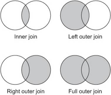
All of these scenarios require you to join datasets together, and the two most common types of joins are inner joins and outer joins. Inner joins compare all tuples in relations L and R, and produce a result if a join predicate is satisfied. In contrast, outer joins don’t require both tuples to match based on a join predicate, and instead can retain a record from L or R even if no match exists. Figure 6.1 illustrates the different types of joins.
Figure 6.1. Different types of joins combining relations, shown as Venn diagrams. The shaded areas show data that is retained in the join.
In this section we’ll look at three joining strategies in MapReduce that support the two most common types of joins (inner and outer). These three strategies perform the join either in the map phase or in the reduce phase by taking advantage of the MapReduce sort-merge architecture:
· Repartition join —A reduce-side join for situations where you’re joining two or more large datasets together
· Replication join —A map-side join that works in situations where one of the datasets is small enough to cache
· Semi-join —Another map-side join where one dataset is initially too large to fit into memory, but after some filtering can be reduced down to a size that can fit in memory
After we cover these joining strategies, we’ll look at a decision tree so you can determine the best join strategy for your situation.
Join data
The techniques will all utilize two datasets to perform the join—users and logs. The user data contains user names, ages, and states. The complete dataset follows:
anne 22 NY
joe 39 CO
alison 35 NY
mike 69 VA
marie 27 OR
jim 21 OR
bob 71 CA
mary 53 NY
dave 36 VA
dude 50 CA
The logs dataset shows some user-based activity that could be extracted from application or webserver logs. The data includes the username, an action, and the source IP address. Here’s the complete dataset:
jim logout 93.24.237.12
mike new_tweet 87.124.79.252
bob new_tweet 58.133.120.100
mike logout 55.237.104.36
jim new_tweet 93.24.237.12
marie view_user 122.158.130.90
jim login 198.184.237.49
marie login 58.133.120.100
Let’s get started by looking at which join method you should pick given your data.
Technique 54 Picking the best join strategy for your data
Each of the join strategies covered in this section has different strengths and weaknesses, and it can be challenging to determine which one is best suited for the data you’re working with. This technique takes a look at different traits in the data and uses that information to pick the optimal approach to join your data.
Problem
You want to select the optimal method to join your data.
Solution
Use a data-driven decision tree to pick the best join strategy.
Discussion
Figure 6.2 shows a decision tree you can use.[1]
1 This decision tree is modeled after the one presented by Spyros Blanas et al., in “A Comparison of Join Algorithms for Log Processing in MapReduce,” http://pages.cs.wisc.edu/~jignesh/publ/hadoopjoin.pdf.
Figure 6.2. Decision tree for selecting a join strategy
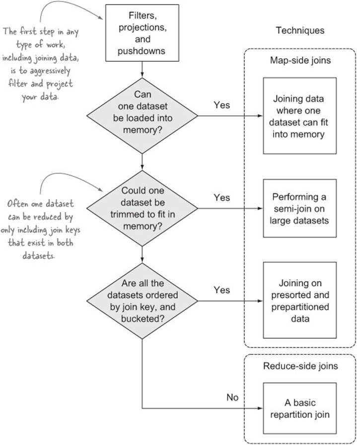
The decision tree can be summarized in the following three points:
· If one of your datasets is small enough to fit into a mapper’s memory, the map-only replicated join is efficient.
· If both datasets are large and one dataset can be substantially reduced by prefiltering elements that don’t match the other, the semi-join works well.
· If you can’t preprocess your data and your data sizes are too large to cache—which means you have to perform the join in the reducer—repartition joins need to be used.
Regardless of which strategy you pick, one of the most fundamental activities you should be performing in your joins is using filters and projections.
Technique 55 Filters, projections, and pushdowns
In this technique, we’ll examine how you can effectively use filters and projections in your mappers to cut down on the amount of data that you’re working with, and spilling, in MapReduce. This technique also examines a more advanced optimization called pushdowns, which can further improve your data pipeline.
Problem
You’re working with large data volumes and you want to efficiently manage your input data to optimize your jobs.
Solution
Filter and project your data to only include the data points you’ll be using in your work.
Discussion
Filtering and projecting data is the biggest optimization you can make when joining data, and when working with data in general. This is a technique that applies to any OLAP activity, and it’s equally effective in Hadoop.
Why are filtering and projection so important? They cut down on the amount of data that a processing pipeline needs to handle. Having less data to work with is important, especially when you’re pushing that data across network and disk boundaries. The shuffle step in MapReduce is expensive because data is being written to local disk and across the network, so having fewer bytes to push around means that your jobs and the MapReduce framework have less work to do, and this translates to faster jobs and less pressure on the CPU, disk, and your networking gear.
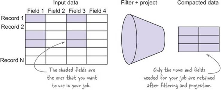
Figure 6.3 shows a simple example of how filtering and projection works.
Figure 6.3. Using filters and projections to reduce data sizes
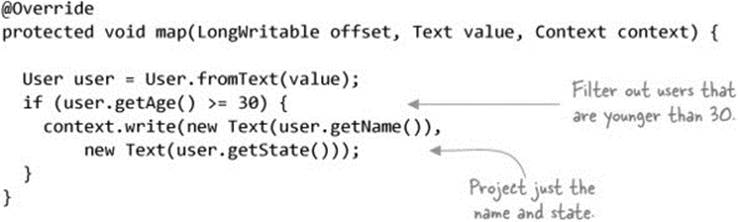
Filters and projections should be performed as close to the data source as possible; in MapReduce this work is best performed in the mappers. The following code shows an example of a filter that excludes users under 30 and only projects their names and states:
The challenge with using filters in joins is that it’s possible that not all of the datasets you’re joining will contain the fields you want to filter on. If this is the case, take a look at technique 61, which discusses using a Bloom filter to help solve this challenge.
Pushdowns
Projection and predicate pushdowns take filtering further by pushing the projections and predicates down to the storage format. This is even more efficient, especially when working with storage formats that can skip over records or entire blocks based on the pushdowns.
Table 6.1 lists the various storage formats and whether they support pushdowns.
Table 6.1. Storage formats and their pushdown support
|
Format |
Projection pushdown supported? |
Predicate pushdown supported? |
|
Text (CSV, JSON, etc.) |
No |
No |
|
Protocol Buffers |
No |
No |
|
Thrift |
No |
No |
|
Avro[a] |
No |
No |
|
Parquet |
Yes |
Yes |
a Avro has both row-major and column-major storage formats.
Further reading on pushdowns
Chapter 3 contains additional details on how Parquet pushdowns can be used in your jobs.
It’s pretty clear that a big advantage of Parquet is its ability to support both types of pushdowns. If you’re working with huge datasets and regularly work on only a subset of the records and fields, then you should consider Parquet as your storage format.
It’s time to move on to the actual joining techniques.
6.1.1. Map-side joins
Our coverage of joining techniques will start with a look at performing joins in the mapper. The reason we’ll cover these techniques first is that they’re the optimal join strategies if your data can support map-side joins. Reduce-size joins are expensive by comparison due to the overhead of shuffling data between the mappers and reducers. As a general policy, map-side joins are preferred.
In this section we’ll look at three different flavors of map-side joins. Technique 56 works well in situations where one of the datasets is already small enough to cache in memory. Technique 57 is more involved, and it also requires that one dataset can fit in memory after filtering out records where the join key exists in both datasets. Technique 58 works in situations where your data is sorted and distributed across your files in a certain way.
Technique 56 Joining data where one dataset can fit into memory
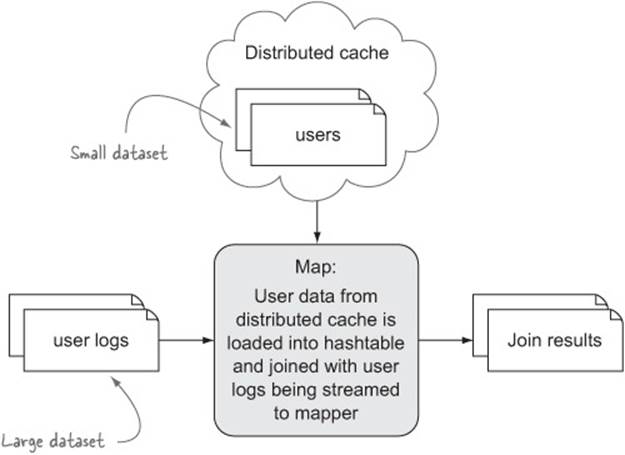
A replicated join is a map-side join, and it gets its name from its function—the smallest of the datasets is replicated to all the map hosts. The replicated join depends on the fact that one of the datasets being joined is small enough to be cached in memory.
Problem
You want to perform a join on data where one dataset can fit into your mapper’s memory.
Solution
Use the distributed cache to cache the smaller dataset and perform the join as the larger dataset is streamed to the mappers.
Discussion
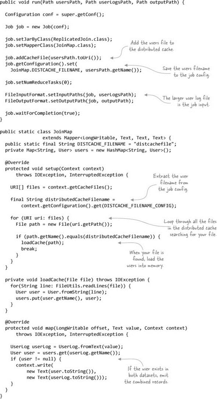
You’ll use the distributed cache to copy the small dataset to the nodes running the map tasks[2] and use the initialization method of each map task to load it into a hashtable. Use the key from each record fed to the map function from the large dataset to look up the small dataset hashtable, and perform a join between the large dataset record and all of the records from the small dataset that match the join value. Figure 6.4 shows how the replicated join works in MapReduce.
2 Hadoop’s distributed cache copies files located on the MapReduce client host or files in HDFS to the slave nodes before any map or reduce tasks are executed on the nodes. Tasks can read these files from their local disk to use as part of their work.
Figure 6.4. Map-only replicated join
The following code performs this join:[3]
3 GitHub source: https://github.com/alexholmes/hiped2/blob/master/src/main/java/hip/ch6/joins/replicated/simple/ReplicatedJoin.java.
To perform this join, you first need to copy the two files you’re going to join to your home directory in HDFS:
$ hadoop fs -put test-data/ch6/users.txt .
$ hadoop fs -put test-data/ch6/user-logs.txt .
Next, run the job and examine its output once it has completed:
$ hip hip.ch6.joins.replicated.simple.ReplicatedJoin \
--users users.txt \
--user-logs user-logs.txt \
--output output
$ hadoop fs -cat output/part*
jim 21 OR jim logout 93.24.237.12
mike 69 VA mike new_tweet 87.124.79.252
bob 71 CA bob new_tweet 58.133.120.100
mike 69 VA mike logout 55.237.104.36
jim 21 OR jim new_tweet 93.24.237.12
marie 27 OR marie view_user 122.158.130.90
jim 21 OR jim login 198.184.237.49
marie 27 OR marie login 58.133.120.100
Hive
Hive joins can be converted to map-side joins by configuring the job prior to execution. It’s important that the largest table be the last table in the query, as that’s the table that Hive will stream in the mapper (the other tables will be cached):
set hive.auto.convert.join=true;
SELECT /*+ MAPJOIN(l) */ u.*, l.*
FROM users u
JOIN user_logs l ON u.name = l.name;
De-emphasizing map-join hint
Hive 0.11 implemented some changes that ostensibly removed the need to supply map-join hints as part of the SELECT statement, but it’s unclear in which situations the hint is no longer needed (see https://issues.apache.org/jira/browse/HIVE-3784).
Map-side joins are not supported for full or right outer joins; they’ll execute as repartition joins (reduce-side joins).
Summary
Both inner and outer joins can be supported with replicated joins. This technique implemented an inner join, because only records that had the same key in both datasets were emitted. To convert this into an outer join, you could emit values being streamed to the mapper that don’t have a corresponding entry in the hashtable, and you could similarly keep track of hashtable entries that were matched with streamed map records and use the cleanup method at the end of the map task to emit records from the hashtable that didn’t match any of the map inputs.
Is there a way to further optimize map-side joins in cases where the dataset is small enough to cache in memory? It’s time to look at semi-joins.
Technique 57 Performing a semi-join on large datasets
Imagine a situation where you’re working with two large datasets that you want to join, such as user logs and user data from an OLTP database. Neither of these datasets is small enough to cache in a map task’s memory, so it would seem you’ll have to resign yourself to performing a reduce-side join. But not necessarily—ask yourself this question: would one of the datasets fit into memory if you were to remove all records that didn’t match a record from the other dataset?
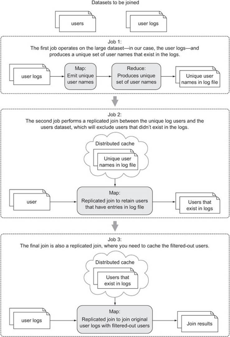
In our example there’s a good chance that the users that appear in your logs are a small percentage of the overall set of users in your OLTP database, so by removing all the OLTP users that don’t appear in your logs, you could get the dataset down to a size that fits into memory. If this is the case, a semi-join is the solution. Figure 6.5 shows the three MapReduce jobs you need to execute to perform a semi-join.
Figure 6.5. The three MapReduce jobs that comprise a semi-join
Let’s look at what’s involved in writing a semi-join.
Problem
You want to join large datasets together and at the same time avoid the overhead of the shuffle and sort phases.
Solution
In this technique you’ll use three MapReduce jobs to join two datasets together to avoid the overhead of a reducer-side join. This technique is useful in situations where you’re working with large datasets, but where a job can be reduced down to a size that can fit into the memory of a task by filtering out records that don’t match the other dataset.
Discussion
In this technique you’ll break down the three jobs illustrated in figure 6.5.
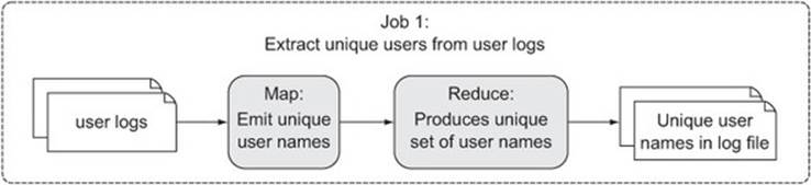
Job 1
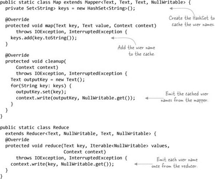
The function of the first MapReduce job is to produce a set of unique user names that exist in the log files. You do this by having the map function perform a projection of the user name, and in turn use the reducers to emit the user name. To cut down on the amount of data transferred between the map and reduce phases, you’ll have the map task cache all of the user names in a HashSet and emit the values of the HashSet in the cleanup method. Figure 6.6 shows the flow of this job.
Figure 6.6. The first job in the semi-join produces a unique set of user names that exist in the log files.
The following code shows the MapReduce job:[4]
4 GitHub source: https://github.com/alexholmes/hiped2/blob/master/src/main/java/hip/ch6/joins/semijoin/UniqueHashedKeyJob.java.
The result of the first job is a unique set of users that appear in the log files.
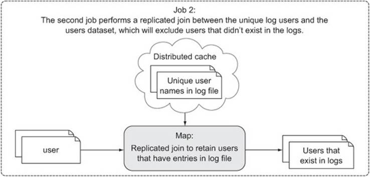
Job 2
The second step is an elaborate filtering MapReduce job, where the goal is to remove users from the user dataset that don’t exist in the log data. This is a map-only job that uses a replicated join to cache the user names that appear in the log files and join them with the user dataset. The unique user output from job 1 will be substantially smaller than the entire user dataset, which makes it the natural selection for caching. Figure 6.7 shows the flow of this job.
Figure 6.7. The second job in the semi-join removes users from the user dataset missing from the log data.
This is a replicated join, just like the one you saw in the previous technique. For that reason I won’t include the code here, but you can easily access it on GitHub.[5]
5 GitHub source: https://github.com/alexholmes/hiped2/blob/master/src/main/java/hip/ch6/joins/semijoin/ReplicatedFilterJob.java.
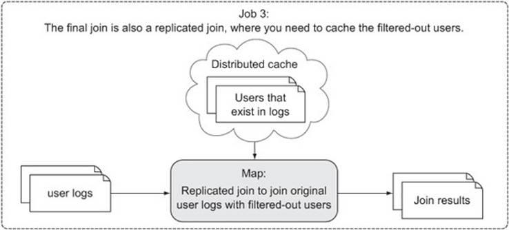
Job 3
In this final step you’ll combine the filtered users produced from job 2 with the original user logs. The filtered users should now be few enough to stick into memory, allowing you to put them in the distributed cache. Figure 6.8 shows the flow of this job.
Figure 6.8. The third job in the semi-join combines the users produced from job 2 with the original user logs.
Again you’re using the replicated join to perform this join, so I won’t show the code for that here—please refer to the previous technique for more details on replicated joins, or go straight to GitHub for the source of this job.[6]
6 GitHub source: https://github.com/alexholmes/hiped2/blob/master/src/main/java/hip/ch6/joins/semijoin/FinalJoinJob.java.
Run the code and look at the output produced by each of the previous steps:
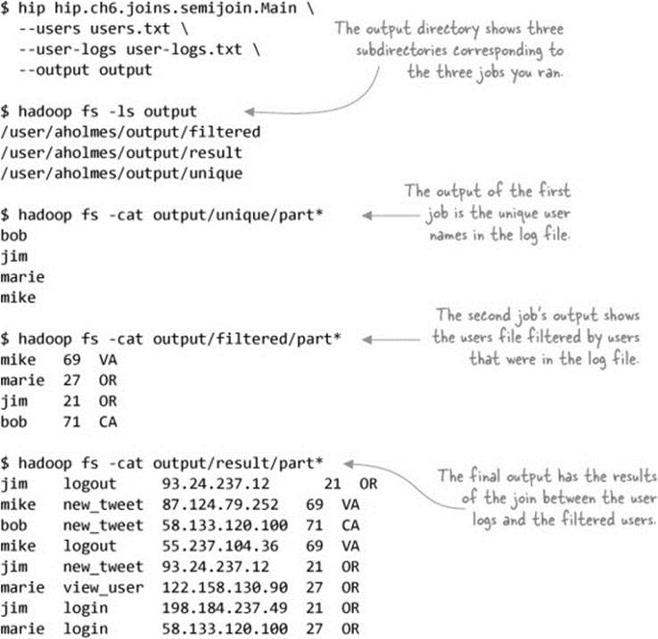
The output shows the logical progression of the jobs in the semi-join and the final join output.
Summary
In this technique we looked at how to use a semi-join to combine two datasets together. The semi-join construct involves more steps than the other joins, but it’s a powerful way to use a map-side join even when working with large datasets (with the caveat that one of the datasets must be reduced to a size that fits in memory).
With these three join strategies in hand, you may be wondering which one you should use in what circumstances.
Technique 58 Joining on presorted and prepartitioned data
Map-side joins are the most efficient techniques, and the previous two map-side strategies both required that one of the datasets could be loaded into memory. What if you’re working with large datasets that can’t be reduced down to a smaller size as required by the previous technique? In this case, a composite map-side join may be viable, but only if all of the following requirements are met:
· None of the datasets can be loaded in memory in its entirety.
· The datasets are all sorted by the join key.
· Each dataset has the same number of files.
· File N in each dataset contains the same join key K.
· Each file is less than the size of an HDFS block, so that partitions aren’t split. Or alternatively, the input split for the data doesn’t split files.
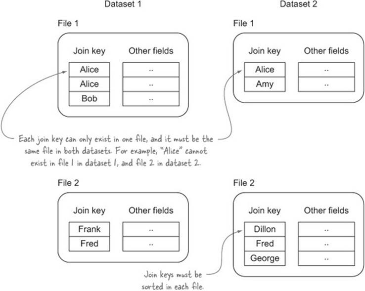
Figure 6.9 shows an example of sorted and partitioned files that lend themselves to composite joins. This technique will look at how you can use the composite join in your jobs.
Figure 6.9. An example of sorted files used as input for the composite join
Problem
You want to perform a map-side join on sorted, partitioned data.
Solution
Use the CompositeInputFormat bundled with MapReduce.
Discussion
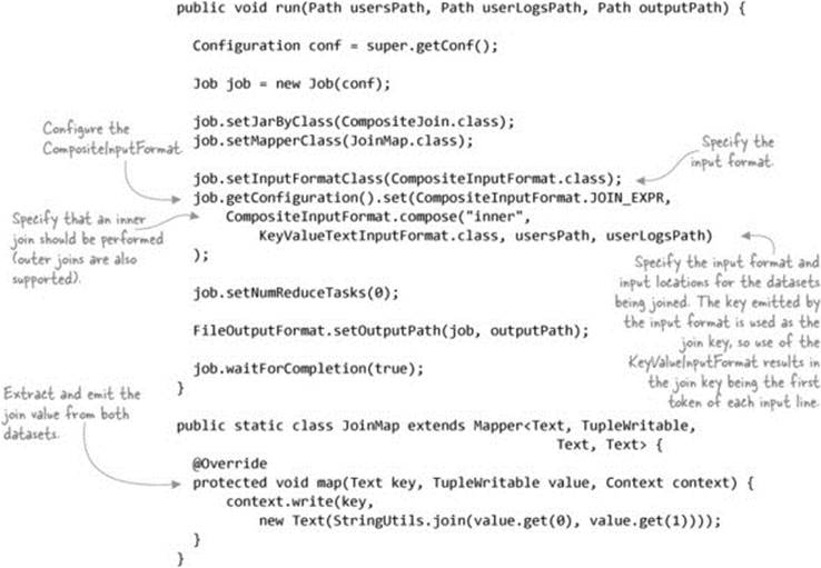
The CompositeInputFormat is quite powerful and supports both inner and outer joins. The following example shows how an inner join would be performed on your data:[7]
7 GitHub source: https://github.com/alexholmes/hiped2/blob/master/src/main/java/hip/ch6/joins/composite/CompositeJoin.java.
The composite join requires the input files to be sorted by key (which is the user name in our example), so before you run the example you’ll need to sort the two files and upload them to HDFS:
$ sort -k1,1 test-data/ch6/users.txt > users-sorted.txt
$ sort -k1,1 test-data/ch6/user-logs.txt > user-logs-sorted.txt
$ hadoop fs -put users-sorted.txt .
$ hadoop fs -put user-logs-sorted.txt .
Next, run the job and examine its output once it has completed:
$ hip hip.ch6.joins.composite.CompositeJoin \
--users users-sorted.txt \
--user-logs user-logs-sorted.txt \
--output output
$ hadoop fs -cat output/part*
bob 71 CA new_tweet 58.133.120.100
jim 21 OR login 198.184.237.49
jim 21 OR logout 93.24.237.12
jim 21 OR new_tweet 93.24.237.12
marie 27 OR login 58.133.120.100
marie 27 OR view_user 122.158.130.90
mike 69 VA logout 55.237.104.36
mike 69 VA new_tweet 87.124.79.252
Hive
Hive supports a map-side join called a sort-merge join, which operates in much the same way as this technique. It also requires all the keys to be sorted in both tables, and the tables must be bucketized into the same number of buckets. You need to specify a number of configurables and also use the MAPJOIN hint to enable this 'margin-top:12.0pt;margin-right:0cm;margin-bottom: 12.0pt;margin-left:8.75pt;line-height:normal'>set hive.input.format=
org.apache.hadoop.hive.ql.io.BucketizedHiveInputFormat;
set hive.optimize.bucketmapjoin = true;
set hive.optimize.bucketmapjoin.sortedmerge = true;
SELECT /*+ MAPJOIN(l) */ u.*, l.*
FROM users u
JOIN user_logs l ON u.name = l.name;
Summary
The composite join actually supports N-way joins, so more than two datasets can be joined. But all datasets must conform to the same set of restrictions that were discussed at the start of this technique.
Because each mapper works with two or more data inputs, data locality can only exist with one of the datasets, so the remaining ones must be streamed from other data nodes.
This join is certainly restrictive in terms of how your data must exist prior to running the join, but if your data is already laid out that way, then this is a good way to join data and avoid the overhead of the shuffle in reducer-based joins.
6.1.2. Reduce-side joins
If none of the map-side techniques work for your data, you’ll need to use the shuffle in MapReduce to sort and join your data together. The following techniques present a number of tips and tricks for your reduce-side joins.
Technique 59 A basic repartition join
The first technique is a basic reduce-side join, which allows you to perform inner and outer joins.
Problem
You want to join together large datasets.
Solution
Use a reduce-side repartition join.
Discussion
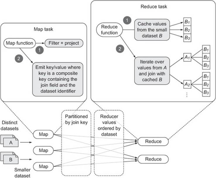
A repartition join is a reduce-side join that takes advantage of MapReduce’s sort-merge to group together records. It’s implemented as a single MapReduce job, and it can support an N-way join, where N is the number of datasets being joined.
The map phase is responsible for reading the data from the various datasets, determining the join value for each record, and emitting that join value as the output key. The output value contains data that you’ll want to include when you combine datasets together in the reducer to produce the job output.
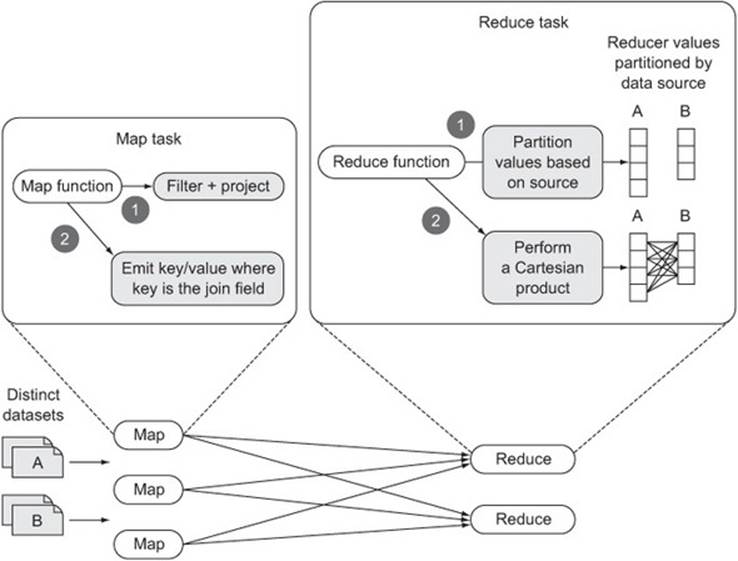
A single reducer invocation receives all of the values for a join key emitted by the map function, and it partitions the data into N partitions, where N is the number of datasets being joined. After the reducer has read all of the input records for the join value and partitioned them in memory, it performs a Cartesian product across all partitions and emits the results of each join. Figure 6.10 shows the repartition join at a high level.
Figure 6.10. A basic MapReduce implementation of a repartition join
There are a number of things that your MapReduce code will need to be able to support for this technique:
· It needs to support multiple map classes, each handling a different input dataset. This is accomplished by using the MultipleInputs class.
· It needs a way to mark records being emitted by the mappers so that they can be correlated with the dataset of their origin. Here you’ll use the htuple project to easily work with composite data in MapReduce.[8]
8 htuple (http://htuple.org) is an open source project that was designed to make it easier to work with tuples in MapReduce. It was created to simplify secondary sorting, which is onerous in MapReduce.
The code for the repartition join follows:[9]
9 GitHub source: https://github.com/alexholmes/hiped2/blob/master/src/main/java/hip/ch6/joins/repartition/SimpleRepartitionJoin.java.
You can use the following commands to run the job and view the job outputs:
$ hip hip.ch6.joins.repartition.SimpleRepartitionJoin \
--users users.txt \
--user-logs user-logs.txt \
--output output
$ hadoop fs -cat output/part*
jim 21 OR jim login 198.184.237.49
jim 21 OR jim new_tweet 93.24.237.12
jim 21 OR jim logout 93.24.237.12
mike 69 VA mike logout 55.237.104.36
mike 69 VA mike new_tweet 87.124.79.252
bob 71 CA bob new_tweet 58.133.120.100
marie 27 OR marie login 58.133.120.100
marie 27 OR marie view_user 122.158.130.90
Summary
Hadoop comes bundled with a hadoop-datajoin module, which is a framework for repartition joins. It includes the main plumbing for handling multiple input datasets and performing the join.
The example shown in this technique as well as the hadoop-datajoin code are the most basic form of repartition joins. Both require that all the data for a join key be loaded into memory before the Cartesian product can be performed. This may work well for your data, but if you have join keys with cardinalities that are larger than your available memory, then you’re out of luck. The next technique looks at a way you can possibly work around this problem.
Technique 60 Optimizing the repartition join
The previous implementation of the repartition join is not space-efficient; it requires all of the output values for a given join value to be loaded into memory before it can perform the multiway join. It’s more efficient to load the smaller of the datasets into memory and then iterate over the larger datasets, performing the join along the way.
Problem
You want to perform a repartition join in MapReduce, but you want to do so without the overhead of caching all the records in the reducer.
Solution
This technique uses an optimized repartition join framework that caches just one of the datasets being joined to reduce the amount of data cached in the reducers.
Discussion
This optimized join only caches records from the smaller of the two datasets to cut down on the memory overhead of caching all the records. Figure 6.11 shows the improved repartition join in action.
Figure 6.11. An optimized MapReduce implementation of a repartition join
There are a few differences between this technique and the simpler repartition join shown in the previous technique. In this technique you’re using a secondary sort to ensure that all the records from the small dataset arrive at the reducer before all the records from the larger dataset. To accomplish this, you’ll emit tuple output keys from the mapper containing the user name being joined on and a field identifying the originating dataset.
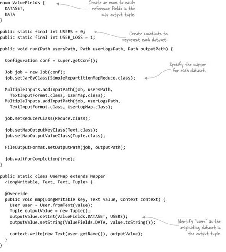
The following code shows a new enum containing the fields that the tuple will contain for the map output keys. It also shows how the user mapper populates the tuple fields:[10]
10 GitHub source: https://github.com/alexholmes/hiped2/blob/master/src/main/java/hip/ch6/joins/repartition/StreamingRepartitionJoin.java.
enum KeyFields {
USER,
DATASET
}
Tuple outputKey = new Tuple();
outputKey.setString(KeyFields.USER, user.getName());
outputKey.setInt(KeyFields.DATASET, USERS);
The MapReduce driver code will need to be updated to indicate which fields in the tuple should be used for sorting, partitioning, and grouping:[11]
11 Secondary sort is covered in more detail in section 6.2.1.
· The partitioner should only partition based on the user name, so that all the records for a user arrive at the same reducer.
· Sorting should use both the user name and dataset indicator, so that the smaller dataset is ordered first (by virtue of the fact that the USERS constant is a smaller number than the USER_LOGS constant, resulting in the user records being sorted before the user logs).
· The grouping should group on users so that both datasets are streamed to the same reducer invocation:
· ShuffleUtils.configBuilder()
· .setPartitionerIndices(KeyFields.USER)
· .setSortIndices(KeyFields.USER, KeyFields.DATASET)
· .setGroupIndices(KeyFields.USER)
.configure(job.getConfiguration());
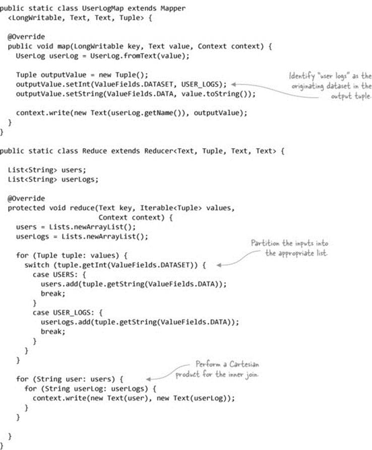
Finally, you’ll modify the reducer to cache the incoming user records, and then join them with the user logs:[12]
12 GitHub source: https://github.com/alexholmes/hiped2/blob/master/src/main/java/hip/ch6/joins/repartition/StreamingRepartitionJoin.java.
@Override
protected void reduce(Tuple key, Iterable<Tuple> values,
Context context){
users = Lists.newArrayList();
for (Tuple tuple : values) {
switch (tuple.getInt(ValueFields.DATASET)) {
case USERS: {
users.add(tuple.getString(ValueFields.DATA));
break;
}
case USER_LOGS: {
String userLog = tuple.getString(ValueFields.DATA);
for (String user : users) {
context.write(new Text(user), new Text(userLog));
}
break;
}
}
}
}
You can use the following commands to run the job and view the job’s output:
$ hip hip.ch6.joins.repartition.StreamingRepartitionJoin \
--users users.txt \
--user-logs user-logs.txt \
--output output
$ hadoop fs -cat output/part*
bob 71 CA bob new_tweet 58.133.120.100
jim 21 OR jim logout 93.24.237.12
jim 21 OR jim new_tweet 93.24.237.12
jim 21 OR jim login 198.184.237.49
marie 27 OR marie view_user 122.158.130.90
marie 27 OR marie login 58.133.120.1
mike 69 VA mike new_tweet 87.124.79.252
mike 69 VA mike logout 55.237.104.36
Hive
Hive can support a similar optimization when performing repartition joins. Hive can cache all the datasets for a join key and then stream the large dataset so that it doesn’t need to be stored in memory.
Hive assumes that the largest dataset is specified last in your query. Imagine you had two tables called users and user_logs, and user_logs was much larger. To join these tables, you’d make sure that the user_logs table was referenced as the last table in the query:
SELECT u.*, l.*
FROM users u
JOIN user_logs l ON u.name = l.name;
If you don’t want to rearrange your query, you can alternatively use the STREAMTABLE hint to tell Hive which table is larger:
SELECT /*+ STREAMTABLE(l) */ u.*, l.*
FROM user_logs l
JOIN users u ON u.name = l.name;
Summary
This join implementation improves on the earlier technique by buffering only the values of the smaller dataset. But it still suffers from the problem of all the data being transmitted between the map and reduce phases, which is an expensive network cost to incur.
Further, the previous technique can support N-way joins, but this implementation only supports two-way joins.
A simple mechanism to reduce further the memory footprint of the reduce-side join is to be aggressive about projections and filters in the map function, as discussed in technique 55.
Technique 61 Using Bloom filters to cut down on shuffled data
Imagine that you wanted to perform a join over a subset of your data according to some predicate, such as “only users that live in California.” With the repartition job techniques covered so far, you’d have to perform that filter in the reducer, because only one dataset (the users) has details about the state—the user logs don’t have that information.
In this technique we’ll look at how a Bloom filter can be used on the map side, which can have a big impact on your job execution time.
Problem
You want to filter data in a repartition join, but to push that filter to the mappers.
Solution
Use a preprocessing job to create a Bloom filter, and then load the Bloom filter in the repartition job to filter out records in the mappers.
Discussion
A Bloom filter is a useful probabilistic data structure that provides membership qualities much like a set—the difference is that membership lookups only provide a definitive “no” answer, as it’s possible to get false positives. Nevertheless, they require a lot less memory compared to a HashSet in Java, so they’re well-suited to work with very large datasets.
More about Bloom filters
Chapter 7 provides details on how Bloom filters work and how to use MapReduce to create a Bloom filter in parallel.
Your goal in this technique is to perform a join only on users that live in California. There are two steps to this solution—you’ll first run a job to generate the Bloom filter, which will operate on the user data and be populated with users that live in California. This Bloom filter will then be used in the repartition join to discard users that don’t exist in the Bloom filter. The reason you need this Bloom filter is that the mapper for the user logs doesn’t have details on the users’ states.
Figure 6.12 shows the steps in this technique.
Figure 6.12. The two-step process to using a Bloom filter in a repartition join
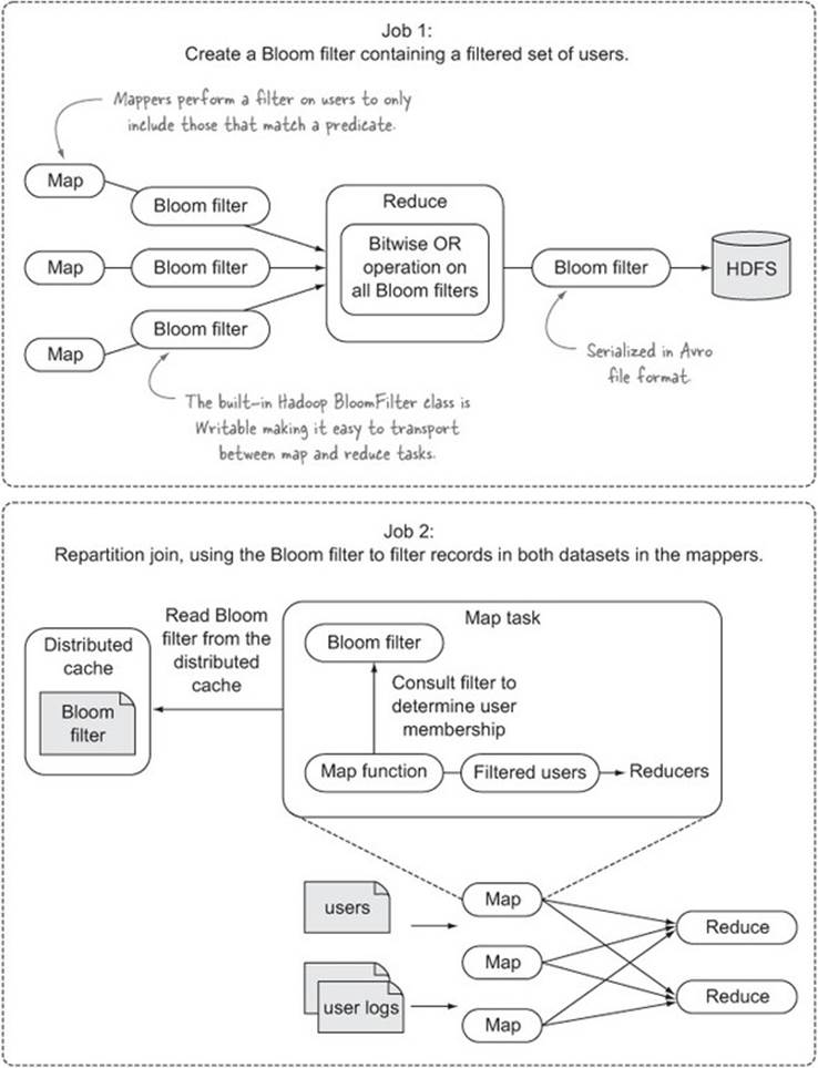
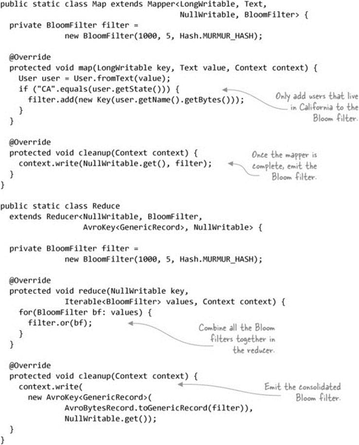
Step 1: Creating the Bloom filter
The first job creates the Bloom filter containing names of users that are in California. The mappers generate intermediary Bloom filters, and the reducer combines them together into a single Bloom filter. The job output is an Avro file containing the serialized Bloom filter:[13]
13 GitHub source: https://github.com/alexholmes/hiped2/blob/master/src/main/java/hip/ch6/joins/bloom/BloomFilterCreator.java.
Step 2: The repartition join
The repartition join is identical to the repartition join presented in technique 59—the only difference is that the mappers now load the Bloom filter generated in the first step, and when processing the map records, they perform a membership query against the Bloom filter to determine whether the record should be sent to the reducer.
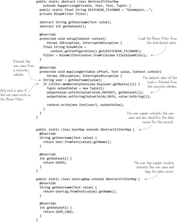
The reducer is unchanged from the original repartition join, so the following code shows two things: the abstract mapper that generalizes the loading of the Bloom filter and the filtering and emission, and the two subclasses that support the two datasets being joined:[14]
14 GitHub source: https://github.com/alexholmes/hiped2/blob/master/src/main/java/hip/ch6/joins/bloom/BloomJoin.java.
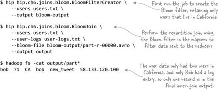
The following commands run the two jobs and dump the output of the join:
Summary
This technique presented an effective method of performing a map-side filter on both datasets to minimize the network I/O between mappers and reducers. It also reduces the amount of data that needs to be spilled to and from disk in both the mappers and reducers as part of the shuffle. Filters are often the simplest and most optimal method of speeding up and optimizing your jobs, and they work just as well for repartition joins as they do for other MapReduce jobs.
Why not use a hashtable rather than a Bloom filter to represent the users? To construct a Bloom filter with a false positive rate of 1%, you need just 9.8 bits for each element in the data structure. Compare this with the best-case use of a HashSet containing integers, which requires 8 bytes. Or if you were to have a HashSet that only reflected the presence of an element that ignores collision, you’d end up with a Bloom filter with a single hash, yielding higher false positives.
Version 0.10 of Pig will include support for Bloom filters in a mechanism similar to that presented here. Details can be viewed in the JIRA ticket at https://issues.apache.org/jira/browse/PIG-2328.
In this section you learned that Bloom filters offer good space-constrained set membership capabilities. We looked at how you could create Bloom filters in Map-Reduce, and you also applied that code to a subsequent technique, which helped you optimize a MapReduce semi-join.
6.1.3. Data skew in reduce-side joins
This section covers a common issue that’s encountered when joining together large datasets—that of data skew. There are two types of data skew that could be present in your data:
· High join-key cardinality, where you have some join keys that have a large number of records in one or both of the datasets. I call this join-product skew.
· Poor hash partitioning, where a minority of reducers receive a large percentage of the overall number of records. I refer to this as hash-partitioning skew.
In severe cases, join-product skews can result in heap exhaustion issues due to the amount of data that needs to be cached. Hash-partitioning skew manifests itself as a join that takes a long time to complete, where a small percentage of the reducers take significantly longer to complete compared to the majority of the reducers.
The techniques in this section examine these two situations and present recommendations for combating them.
Technique 62 Joining large datasets with high join-key cardinality
This technique tackles the problem of join-product skew, and the next technique examines hash-partitioning skew.
Problem
Some of your join keys are high-cardinality, which results in some of your reducers running out of memory when trying to cache these keys.
Solution
Filter out these keys and join them separately or spill them out in the reducer and schedule a follow-up job to join them.
Discussion
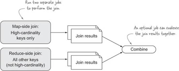
If you know ahead of time which keys are high-cardinality, you can separate them out into a separate join job, as shown in figure 6.13.
Figure 6.13. Dealing with skew when you know the high-cardinality key ahead of time
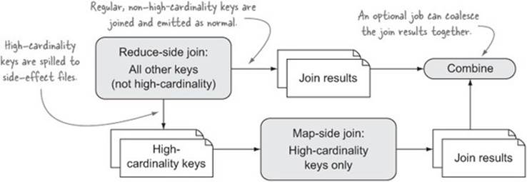
If you don’t know the high-cardinality keys, you may have to build some intelligence into your reducers to detect these keys and write them out to a side-effect file, which is joined by a subsequent job, as illustrated in figure 6.14.
Figure 6.14. Dealing with skew when you don’t know high-cardinality keys ahead of time
Hive 0.13
The skewed key implementation was flawed in Hive versions before 0.13 (https://issues.apache.org/jira/browse/HIVE-6041).
Hive
Hive supports a skew-mitigation strategy similar to the second approach presented in this technique. It can be enabled by specifying the following configurables prior to running the job:
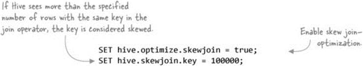
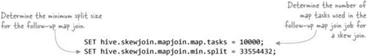
You can optionally set some additional configurables to control the map-side join that operates on the high-cardinality keys:
Finally, if you’re using a GROUP BY in your SQL, you may also want to consider enabling the following configuration to handle skews in the grouped data:
SET hive.groupby.skewindata = true;
Summary
The options presented in this technique assume that for a given join key, only one dataset has high-cardinality occurrences; hence the use of a map-side join that caches the smaller of the datasets. If both datasets are high-cardinality, then you’re facing an expensive Cartesian product operation that will be slow to execute, as it doesn’t lend itself to the MapReduce way of doing work (meaning it’s not inherently splittable and parallelizable). In this case, you are essentially out of options in terms of optimizing the actual join. You should reexamine whether any back-to-basics techniques, such as filtering or projecting your data, can help alleviate the time required to execute the join.
The next technique looks at a different type of skew that can be introduced into your application as a result of using the default hash partitioner.
Technique 63 Handling skews generated by the hash partitioner
The default partitioner in MapReduce is a hash partitioner, which takes a hash of each map output key and performs a modulo against the number of reducers to determine the reducer the key is sent to. The hash partitioner works well as a general partitioner, but it’s possible that some datasets will cause the hash partitioner to overload some reducers due to a disproportionate number of keys being hashed to the same reducer.
This is manifested by a small number of straggling reducers taking much longer to complete compared to the majority of reducers. In addition, when you examine the straggler reducer counters, you’ll notice that the number of groups sent to the stragglers is much higher than the others that have completed.
Differentiating between skew caused by high-cardinality keys versus a hash partitioner
You can use the MapReduce reducer counters to identify the type of data skew in your job. Skews introduced by a poorly performing hash partitioner will have a much higher number of groups (unique keys) sent to these reducers, whereas the symptoms of high-cardinality keys causing skew is evidenced by the roughly equal number of groups across all reducers but a much higher number of records for skewed reducers.
Problem
Your reduce-side joins are taking a long time to complete, with several straggler reducers taking significantly longer to complete than the majority.
Solution
Use a range partitioner or write a custom partitioner that siphons skewed keys to a reserved set of reducers.
Discussion
The goal of this solution is to dispense with the default hash partitioner and replace it with something that works better with your skewed data. There are two options you can explore here:
· You can use the sampler and TotalOrderPartitioner that comes bundled with Hadoop, which replaces the hash partitioner with a range partitioner.
· You can write a custom partitioner that routes keys with data skew to a set of reducers reserved for skewed keys.
Let’s explore both options and look at how you’d use them.
Range partitioning
A range partitioner will distribute map outputs based on a predefined range of values, where each range maps to a reducer that will receive all outputs within that range. This is exactly how the TotalOrderPartitioner works. In fact, the TotalOrderPartitioner is used by TeraSort to evenly distribute words across all the reducers to minimize straggling reducers.[15]
15 TeraSort is a Hadoop benchmarking tool that sorts a terabyte of data.
For range partitioners such as the TotalOrderPartitioner to do their work, they need to know the output key ranges for a given job. The TotalOrderPartitioner is accompanied by a sampler that samples the input data and writes these ranges to HDFS, which is then used by theTotalOrderPartitioner when partitioning. More details on how to use the TotalOrderPartitioner and the sampler are covered in section 6.2.
Custom partitioner
If you already have a handle on which keys exhibit data skew, and that set of keys is static, you can write a custom partitioner to push these high-cardinality join keys to a reserved set of reducers. Imagine that you’re running a job with ten reducers—you could decide to use two of them for keys that are skewed, and then hash partition all other keys across the remainder of the reducers.
Summary
Of the two approaches presented here, range partitioning is quite possibly the best solution, as it’s likely that you won’t know which keys are skewed, and it’s also possible that the keys that exhibit skew will change over time.
It’s possible to have reduce-side joins in MapReduce because they sort and correlate the map output keys together. In the next section, we’ll look at common sorting techniques in MapReduce.
6.2. Sorting
The magic of MapReduce occurs between the mappers and reducers, where the framework groups together all the map output records that were emitted with the same key. This MapReduce feature allows you to aggregate and join your data and implement powerful data pipelines. To execute this feature, MapReduce internally partitions, sorts, and merges data (which is part of the shuffle phase), and the result is that each reducer is streamed an ordered set of keys and accompanying values.
In this section we’ll explore two particular areas where you’ll want to tweak the behavior of MapReduce sorting.
First we’ll look at the secondary sort, which allows you to sort values for a reducer key. Secondary sorts are useful when you want some data to arrive at your reducer ahead of other data, as in the case of the optimized repartition join in technique 60. Secondary sorts are also useful if you want your job output to be sorted by a secondary key. An example of this is if you want to perform a primary sort of stock data by stock symbol, and then perform a secondary sort on the time of each stock quote during a day.
The second scenario we’ll cover in this section is sorting data across all the reducer outputs. This is useful in situations where you want to extract the top or bottom N elements from a dataset.
These are important areas that allow you to perform some of the joins that we looked at earlier in this chapter. But the applicability of sorting isn’t limited to joins; sorting also allows you to provide a secondary sort over your data. Secondary sorts are used in many of the techniques in this book, ranging from optimizing the repartition join to graph algorithms such as friends-of-friends.
6.2.1. Secondary sort
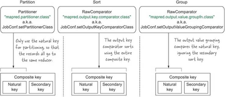
As you saw in the discussion of joining in section 6.1, you need secondary sorts to allow some records to arrive at a reducer ahead of other records. Secondary sorts require an understanding of both data arrangement and data flows in MapReduce. Figure 6.15 shows the three elements that affect data arrangement and flow (partitioning, sorting, and grouping) and how they’re integrated into MapReduce.
Figure 6.15. An overview of where sorting, partitioning, and grouping occur in MapReduce
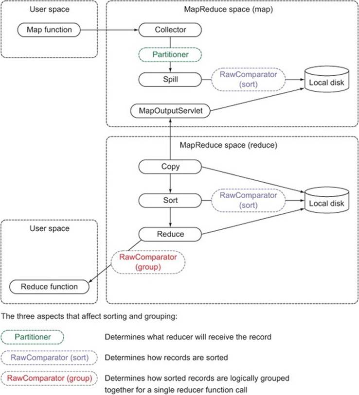
The partitioner is invoked as part of the map output collection process, and it’s used to determine which reducer should receive the map output. The sorting RawComparator is used to sort the map outputs within their respective partitions, and it’s used in both the map and reduce sides. Finally, the grouping RawComparator is responsible for determining the group boundaries across the sorted records.
The default behavior in MapReduce is for all three functions to operate on the entire output key emitted by map functions.
Technique 64 Implementing a secondary sort
Secondary sorts are useful when you want some of the values for a unique map key to arrive at a reducer ahead of other values. You can see the value of secondary sorting in other techniques in this book, such as the optimized repartition join (technique 60), and the friends-of-friends algorithm discussed in chapter 7 (technique 68).
Problem
You want to order values sent to a single reducer invocation for each key.
Solution
This technique covers writing your partitioner, sort comparator, and grouping comparator classes, which are required for secondary sorting to work.
Discussion
In this technique we’ll look at how to use secondary sorts to order people’s names. You’ll use the primary sort to order people’s last names, and the secondary sort to order their first names.
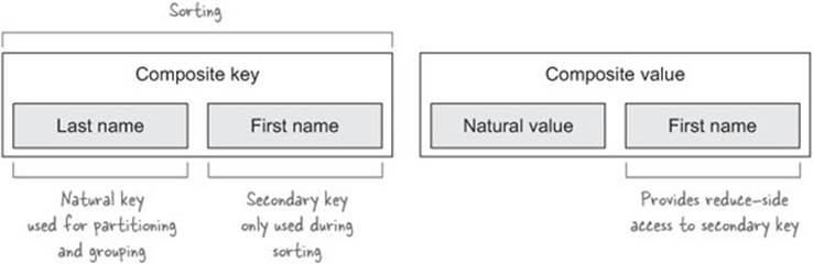
To support secondary sort, you need to create a composite output key, which will be emitted by your map functions. The composite key will contain two parts:
· The natural key, which is the key to use for joining purposes
· The secondary key, which is the key to use to order all of the values sent to the reducer for the natural key
Figure 6.16 shows the composite key for the names. It also shows a composite value that provides reducer-side access to the secondary key.
Figure 6.16. The user composite key and value
Let’s go through the partitioning, sorting, and grouping phases and implement them to sort the names. But before that, you need to write your composite key class.
Composite key
The composite key contains both the first and last name. It extends WritableComparable, which is recommended for Writable classes that are emitted as keys from map functions:[16]
16 GitHub source: https://github.com/alexholmes/hiped2/blob/master/src/main/java/hip/ch6/sort/secondary/Person.java.
public class Person implements WritableComparable<Person> {
private String firstName;
private String lastName;
@Override
public void readFields(DataInput in) throws IOException {
this.firstName = in.readUTF();
this.lastName = in.readUTF();
}
@Override
public void write(DataOutput out) throws IOException {
out.writeUTF(firstName);
out.writeUTF(lastName);
}
...
Figure 6.17 shows the configuration names and methods that you’ll call in your code to set the partitioning, sorting, and grouping classes. The figure also shows what part of the composite key each class uses.
Figure 6.17. Partitioning, sorting, and grouping settings and key utilization
Let’s look at the implementation code for each of these classes.
Partitioner
The partitioner is used to determine which reducer should receive a map output record. The default MapReduce partitioner (HashPartitioner) calls the hashCode method of the output key and performs a modulo with the number of reducers to determine which reducer should receive the output. The default partitioner uses the entire key, which won’t work for your composite key, because it will likely send keys with the same natural key value to different reducers. Instead, you need to write your own Partitioner that partitions on the natural key.
The following code shows the Partitioner interface you must implement. The getPartition method is passed the key, value, and number of partitions (also known as reducers):
public interface Partitioner<K2, V2> extends JobConfigurable {
int getPartition(K2 key, V2 value, int numPartitions);
}
Your partitioner will calculate a hash based on the last name in the Person class and perform a modulo of that with the number of partitions (which is the number of reducers):[17]
17 GitHub source: https://github.com/alexholmes/hiped2/blob/master/src/main/java/hip/ch6/sort/secondary/PersonNamePartitioner.java.
public class PersonNamePartitioner extends
Partitioner<Person, Text> {
@Override
public int getPartition(Person key, Text value, int numPartitions) {
return Math.abs(key.getLastName().hashCode() * 127) %
numPartitions;
}
}
Sorting
Both the map and reduce sides participate in sorting. The map-side sorting is an optimization to help make the reducer sorting more efficient. You want MapReduce to use your entire key for sorting purposes, which will order keys according to both the last name and the first name.
In the following example, you can see the implementation of the WritableComparator, which compares users based on their last name and their first name:[18]
18 GitHub source: https://github.com/alexholmes/hiped2/blob/master/src/main/java/hip/ch6/sort/secondary/PersonComparator.java.
public class PersonComparator extends WritableComparator {
protected PersonComparator() {
super(Person.class, true);
}
@Override
public int compare(WritableComparable w1, WritableComparable w2) {
Person p1 = (Person) w1;
Person p2 = (Person) w2;
int cmp = p1.getLastName().compareTo(p2.getLastName());
if (cmp != 0) {
return cmp;
}
return p1.getFirstName().compareTo(p2.getFirstName());
}
}
Grouping
Grouping occurs when the reduce phase is streaming map output records from local disk. Grouping is the process by which you can specify how records are combined to form one logical sequence of records for a reducer invocation.
When you’re at the grouping stage, all of the records are already in secondary-sort order, and the grouping comparator needs to bundle together records with the same last name:[19]
19 GitHub source: https://github.com/alexholmes/hiped2/blob/master/src/main/java/hip/ch6/sort/secondary/PersonNameComparator.java.
public class PersonNameComparator extends WritableComparator {
protected PersonNameComparator() {
super(Person.class, true);
}
@Override
public int compare(WritableComparable o1, WritableComparable o2) {
Person p1 = (Person) o1;
Person p2 = (Person) o2;
return p1.getLastName().compareTo(p2.getLastName());
}
}
MapReduce
The final steps involve telling MapReduce to use the partitioner, sort comparator, and group comparator classes:[20]
20 GitHub source: https://github.com/alexholmes/hiped2/blob/master/src/main/java/hip/ch6/sort/secondary/SortMapReduce.java.
job.setPartitionerClass(PersonNamePartitioner.class);
job.setSortComparatorClass(PersonComparator.class);
job.setGroupingComparatorClass(PersonNameComparator.class);
To complete this technique, you need to write the map and reduce code. The mapper creates the composite key and emits that in conjunction with the first name as the output value. The reducer produces output identical to the input:[21]
21 GitHub source: https://github.com/alexholmes/hiped2/blob/master/src/main/java/hip/ch6/sort/secondary/SortMapReduce.java.
public static class Map extends Mapper<Text, Text, Person, Text> {
private Person outputKey = new Person();
@Override
protected void map(Text lastName, Text firstName, Context context)
throws IOException, InterruptedException {
outputKey.set(lastName.toString(), firstName.toString());
context.write(outputKey, firstName);
}
}
public static class Reduce extends Reducer<Person, Text, Text, Text> {
Text lastName = new Text();
@Override
public void reduce(Person key, Iterable<Text> values,
Context context)
throws IOException, InterruptedException {
lastName.set(key.getLastName());
for (Text firstName : values) {
context.write(lastName, firstName);
}
}
}
To see this sort in action, you can upload a small file with unordered names and test whether the secondary sort code produces output sorted by first name:
$ hadoop fs -put test-data/ch6/usernames.txt .
$ hadoop fs -cat usernames.txt
Smith John
Smith Anne
Smith Ken
$ hip hip.ch6.sort.secondary.SortMapReduce \
--input usernames.txt --output output
$ hadoop fs -cat output/part*
Smith Anne
Smith John
Smith Ken
The output is sorted as expected.
Summary
As you can see in this technique, it’s nontrivial to use secondary sort. It requires you to write a custom partitioner, sorter, and grouper. If you’re working with simple data types, consider using htuple (http://htuple.org/), an open source project I developed, which simplifies secondary sort in your jobs.
htuple exposes a Tuple class, which allows you to store one or more Java types and provides helper methods to make it easy for you to define which fields are used for partitioning, sorting, and grouping. The following code shows how htuple can be used to secondary sort on the first name, just like in the technique:
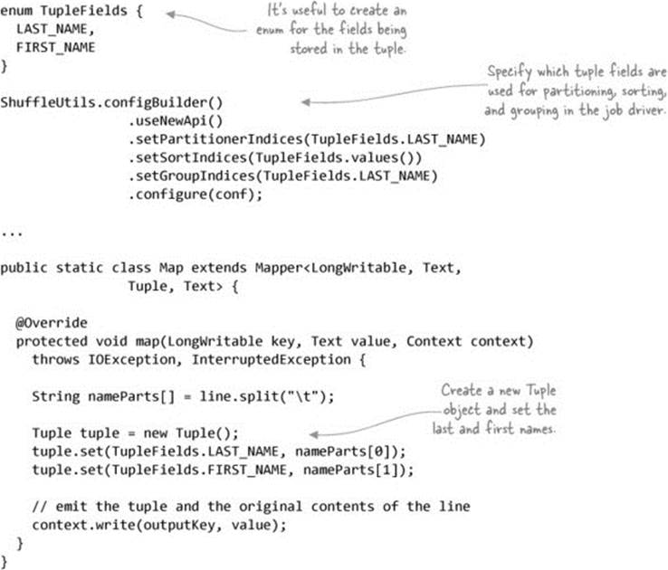
Next we’ll look at how to sort outputs across multiple reducers.
6.2.2. Total order sorting
You’ll find a number of situations where you’ll want to have your job output in total sort order.[22] For example, if you want to extract the most popular URLs from a web graph, you’ll have to order your graph by some measure of popularity, such as Page-Rank. Or if you want to display a table in your portal of the most active users on your site, you’ll need the ability to sort them based on some criteria, such as the number of articles they wrote.
22 Total sort order is when the reducer records are sorted across all the reducers, not just within each reducer.
Technique 65 Sorting keys across multiple reducers
You know that the MapReduce framework sorts map output keys prior to feeding them to reducers. But this sorting is only guaranteed within each reducer, and unless you specify a partitioner for your job, you’ll be using the default MapReduce partitioner, HashPartitioner, which partitions using a hash of the map output keys. This ensures that all records with the same map output key go to the same reducer, but the HashPartitioner doesn’t perform total sorting of the map output keys across all the reducers. Knowing this, you may be wondering how you could use Map-Reduce to sort keys across multiple reducers so that you can easily extract the top and bottom N records from your data.
Problem
You want a total ordering of keys in your job output, but without the overhead of having to run a single reducer.
Solution
This technique covers use of the TotalOrderPartitioner class, a partitioner that is bundled with Hadoop, to assist in sorting output across all reducers. The partitioner ensures that output sent to the reducers is totally ordered.
Discussion
Hadoop has a built-in partitioner called the TotalOrderPartitioner, which distributes keys to specific reducers based on a partition file. The partition file is a precomputed SequenceFile that contains N – 1 keys, where N is the number of reducers. The keys in the partition file are ordered by the map output key comparator, and as such, each key represents a logical range of keys. To determine which reducer should receive an output record, the TotalOrderPartitioner examines the output key, determines which range it falls into, and maps that range into a specific reducer.
Figure 6.18 shows the two parts of this technique. You need to create the partition file and then run your MapReduce job using the TotalOrderPartitioner.
Figure 6.18. Using sampling and the TotalOrderPartitioner to sort output across all reducers.
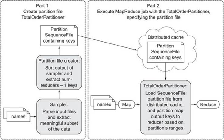
First you’ll use the InputSampler class, which samples the input files and creates the partition file. You can use one of two samplers: the RandomSampler class, which as the name suggests picks random records from the input, or the IntervalSampler class, which for every record includes the record in the sample. Once the samples have been extracted, they’re sorted, and then N – 1 keys are written to the partition file, where N is the number of reducers. The InputSampler isn’t a MapReduce job; it reads records from the InputFormat and produces the partition within the process calling the code.
The following code shows the steps you need to execute prior to calling the InputSampler function:[23]
23 GitHub source: https://github.com/alexholmes/hiped2/blob/master/src/main/java/hip/ch6/sort/total/TotalSortMapReduce.java.
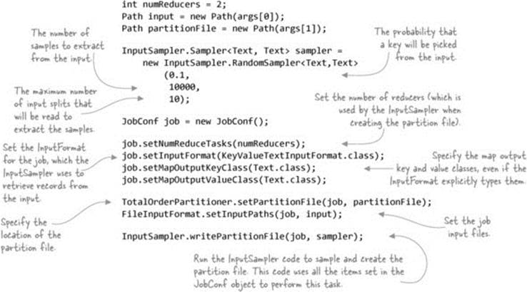
Next up, you need to specify that you want to use the TotalOrderPartitioner as the partitioner for your job:
job.setPartitionerClass(TotalOrderPartitioner.class);
You don’t want to do any processing in your MapReduce job, so you won’t specify the map or reduce classes. This means the identity MapReduce classes will be used, so you’re ready to run the code:
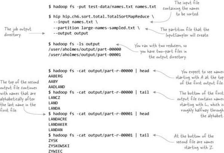
You can see from the results of the MapReduce job that the map output keys are indeed sorted across all the output files.
Summary
This technique used the InputSampler to create the partition file, which is subsequently used by the TotalOrderPartitioner to partition map output keys.
You could also use MapReduce to generate the partition file. An efficient way of doing this would be to write a custom InputFormat class that performs the sampling and then output the keys to a single reducer, which in turn can create the partition file. This brings us to sampling, the last section of this chapter.
6.3. Sampling
Imagine you’re working with a terabyte-scale dataset, and you have a MapReduce application you want to test with that dataset. Running your MapReduce application against the dataset may take hours, and constantly making code refinements and rerunning against the large dataset isn’t an optimal workflow.
To solve this problem, you look to sampling, which is a statistical methodology for extracting a relevant subset of a population. In the context of MapReduce, sampling provides an opportunity to work with large datasets without the overhead of having to wait for the entire dataset to be read and processed. This greatly enhances your ability to quickly iterate when developing and debugging MapReduce code.
Technique 66 Writing a reservoir-sampling InputFormat
You’re developing a MapReduce job iteratively with a large dataset, and you need to do testing. Testing with the entire dataset takes a long time and impedes your ability to rapidly work with your code.
Problem
You want to work with a small subset of a large dataset during the development of a MapReduce job.
Solution
Write an input format that can wrap the actual input format used to read data. The input format that you’ll write can be configured with the number of samples that should be extracted from the wrapped input format.
Discussion
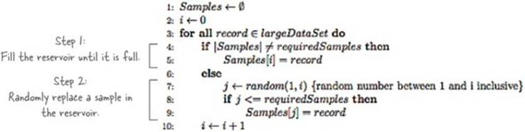
In this technique you’ll use reservoir sampling to choose samples. Reservoir sampling is a strategy that allows a single pass through a stream to randomly produce a sample.[24] As such, it’s a perfect fit for MapReduce because input records are streamed from an input source. Figure 6.19shows the algorithm for reservoir sampling.
24 For more information on reservoir sampling, see the Wikipedia article at http://en.wikipedia.org/wiki/Reservoir_sampling.
Figure 6.19. The reservoir-sampling algorithm allows one pass through a stream to randomly produce a sample.
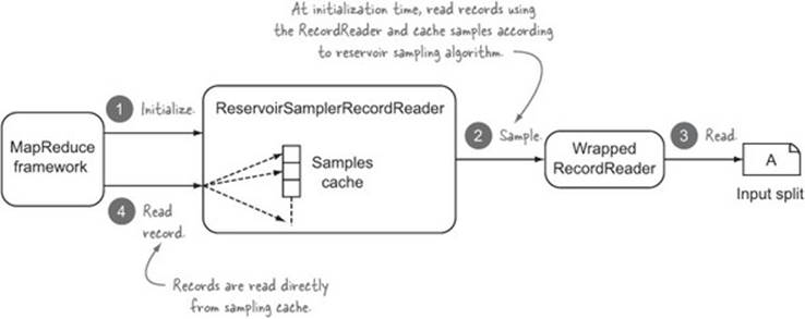
The input split determination and record reading will be delegated to wrapped InputFormat and RecordReader classes. You’ll write classes that provide the sampling functionality and then wrap the delegated InputFormat and RecordReader classes.[25] Figure 6.20 shows how theReservoirSamplerRecordReader works.
25 If you need a refresher on these classes, please review chapter 3 for more details.
Figure 6.20. The ReservoirSamplerRecordReader in action
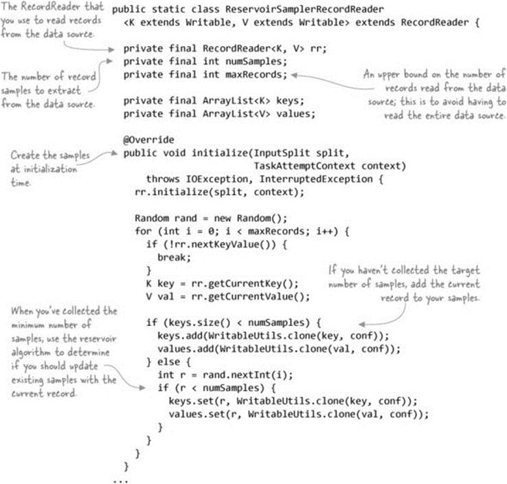
The following code shows the ReservoirSamplerRecordReader:[26]
26 GitHub source: https://github.com/alexholmes/hiped2/blob/master/src/main/java/hip/ch6/sampler/ReservoirSamplerInputFormat.java.
To use the ReservoirSamplerInputFormat class in your code, you’ll use convenience methods to help set up the input format and other parameters, as shown in the following code:[27]
27 GitHub source: https://github.com/alexholmes/hiped2/blob/master/src/main/java/hip/ch6/sampler/SamplerJob.java
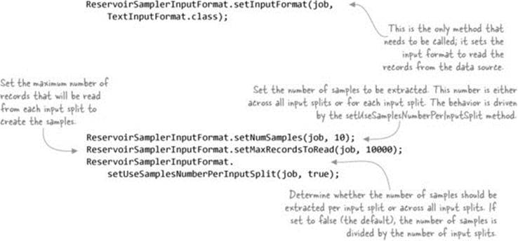
You can see the sampling input format in action by running an identity job against a large file containing names:
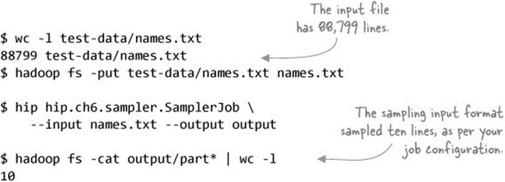
You configured the ReservoirSamplerInputFormat to extract ten samples, and the output file contained that number of lines.
Summary
Sampling support in MapReduce code can be a useful development and testing feature when engineers are running code against production-scale datasets. That begs the question: what’s the best approach for integrating sampling support into an existing codebase? One approach would be to add a configurable option that would toggle the use of the sampling input format, similar to the following code:
if(appConfig.isSampling()) {
ReservoirSamplerInputFormat.setInputFormat(job,
TextInputFormat.class);
...
} else {
job.setInputFormatClass(TextInputFormat.class);
}
You can apply this sampling technique to any of the preceding sections as a way to work efficiently with large datasets.
6.4. Chapter summary
Joining and sorting are cumbersome tasks in MapReduce, and we spent this chapter discussing methods to optimize and facilitate their use. We looked at three different join strategies, two of which were on the map side, and one on the reduce side. The goal was to simplify joins in MapReduce, and I presented two frameworks that reduce the amount of user code required for joins.
We also covered sorting in MapReduce by examining how secondary sorts work and how you can sort all of the output across all the reducers. And we wrapped things up with a look at how you can sample data so that you can quickly iterate over smaller samples of your data.
We’ll cover a number of performance patterns and tuning steps in chapter 8, which will result in faster join and sorting times. But before we get there, we’ll look at some more advanced data structures and algorithms, such as graph processing and working with Bloom filters.