Hadoop: The Definitive Guide (2015)

Part II. MapReduce

Chapter 9. MapReduce Features

This chapter looks at some of the more advanced features of MapReduce, including counters and sorting and joining datasets.

Counters

There are often things that you would like to know about the data you are analyzing but that are peripheral to the analysis you are performing. For example, if you were counting invalid records and discovered that the proportion of invalid records in the whole dataset was very high, you might be prompted to check why so many records were being marked as invalid — perhaps there is a bug in the part of the program that detects invalid records? Or if the data was of poor quality and genuinely did have very many invalid records, after discovering this, you might decide to increase the size of the dataset so that the number of good records was large enough for meaningful analysis.

Counters are a useful channel for gathering statistics about the job: for quality control or for application-level statistics. They are also useful for problem diagnosis. If you are tempted to put a log message into your map or reduce task, it is often better to see whether you can use a counter instead to record that a particular condition occurred. In addition to counter values being much easier to retrieve than log output for large distributed jobs, you get a record of the number of times that condition occurred, which is more work to obtain from a set of logfiles.

Built-in Counters

Hadoop maintains some built-in counters for every job, and these report various metrics. For example, there are counters for the number of bytes and records processed, which allow you to confirm that the expected amount of input was consumed and the expected amount of output was produced.

Counters are divided into groups, and there are several groups for the built-in counters, listed in Table 9-1.

Table 9-1. Built-in counter groups

Each group either contains task counters (which are updated as a task progresses) or job counters (which are updated as a job progresses). We look at both types in the following sections.

Task counters

Task counters gather information about tasks over the course of their execution, and the results are aggregated over all the tasks in a job. The MAP_INPUT_RECORDS counter, for example, counts the input records read by each map task and aggregates over all map tasks in a job, so that the final figure is the total number of input records for the whole job.

Task counters are maintained by each task attempt, and periodically sent to the application master so they can be globally aggregated. (This is described in Progress and Status Updates.) Task counters are sent in full every time, rather than sending the counts since the last transmission, since this guards against errors due to lost messages. Furthermore, during a job run, counters may go down if a task fails.

Counter values are definitive only once a job has successfully completed. However, some counters provide useful diagnostic information as a task is progressing, and it can be useful to monitor them with the web UI. For example, PHYSICAL_MEMORY_BYTES, VIRTUAL_MEMORY_BYTES, andCOMMITTED_HEAP_BYTES provide an indication of how memory usage varies over the course of a particular task attempt.

The built-in task counters include those in the MapReduce task counters group (Table 9-2) and those in the file-related counters groups (Tables 9-3, 9-4, and 9-5).

Table 9-2. Built-in MapReduce task counters

Table 9-3. Built-in filesystem task counters

Table 9-4. Built-in FileInputFormat task counters

Table 9-5. Built-in FileOutputFormat task counters

Job counters

Job counters (Table 9-6) are maintained by the application master, so they don’t need to be sent across the network, unlike all other counters, including user-defined ones. They measure job-level statistics, not values that change while a task is running. For example,TOTAL_LAUNCHED_MAPS counts the number of map tasks that were launched over the course of a job (including tasks that failed).

Table 9-6. Built-in job counters

User-Defined Java Counters

MapReduce allows user code to define a set of counters, which are then incremented as desired in the mapper or reducer. Counters are defined by a Java enum, which serves to group related counters. A job may define an arbitrary number of enums, each with an arbitrary number of fields. The name of the enum is the group name, and the enum’s fields are the counter names. Counters are global: the MapReduce framework aggregates them across all maps and reduces to produce a grand total at the end of the job.

We created some counters in Chapter 6 for counting malformed records in the weather dataset. The program in Example 9-1 extends that example to count the number of missing records and the distribution of temperature quality codes.

Example 9-1. Application to run the maximum temperature job, including counting missing and malformed fields and quality codes

public class MaxTemperatureWithCounters extends Configured implements Tool {

enum Temperature {

MISSING,

MALFORMED

}

static class MaxTemperatureMapperWithCounters

extends Mapper<LongWritable, Text, Text, IntWritable> {

private NcdcRecordParser parser = new NcdcRecordParser();

@Override

protected void map(LongWritable key, Text value, Context context)

throws IOException, InterruptedException {

parser.parse(value);

if (parser.isValidTemperature()) {

int airTemperature = parser.getAirTemperature();

context.write(new Text(parser.getYear()),

new IntWritable(airTemperature));

} else if (parser.isMalformedTemperature()) {

System.err.println("Ignoring possibly corrupt input: " + value);

context.getCounter(Temperature.MALFORMED).increment(1);

} else if (parser.isMissingTemperature()) {

context.getCounter(Temperature.MISSING).increment(1);

}

// dynamic counter

context.getCounter("TemperatureQuality", parser.getQuality()).increment(1);

}

}

@Override

public int run(String[] args) throws Exception {

Job job = JobBuilder.parseInputAndOutput(this, getConf(), args);

if (job == null) {

return -1;

}

job.setOutputKeyClass(Text.class);

job.setOutputValueClass(IntWritable.class);

job.setMapperClass(MaxTemperatureMapperWithCounters.class);

job.setCombinerClass(MaxTemperatureReducer.class);

job.setReducerClass(MaxTemperatureReducer.class);

return job.waitForCompletion(true) ? 0 : 1;

}

public static void main(String[] args) throws Exception {

int exitCode = ToolRunner.run(new MaxTemperatureWithCounters(), args);

System.exit(exitCode);

}

}

The best way to see what this program does is to run it over the complete dataset:

% hadoop jar hadoop-examples.jar MaxTemperatureWithCounters \

input/ncdc/all output-counters

When the job has successfully completed, it prints out the counters at the end (this is done by the job client). Here are the ones we are interested in:

Air Temperature Records

Malformed=3

Missing=66136856

TemperatureQuality

0=1

1=973422173

2=1246032

4=10764500

5=158291879

6=40066

9=66136858

Notice that the counters for temperature have been made more readable by using a resource bundle named after the enum (using an underscore as a separator for nested classes) — in this case MaxTemperatureWithCounters_Temperature.properties, which contains the display name mappings.

Dynamic counters

The code makes use of a dynamic counter — one that isn’t defined by a Java enum. Because a Java enum’s fields are defined at compile time, you can’t create new counters on the fly using enums. Here we want to count the distribution of temperature quality codes, and though the format specification defines the values that the temperature quality code can take, it is more convenient to use a dynamic counter to emit the values that it actually takes. The method we use on the Context object takes a group and counter name using String names:

public Counter getCounter(String groupName, String counterName)

The two ways of creating and accessing counters — using enums and using strings — are actually equivalent because Hadoop turns enums into strings to send counters over RPC. Enums are slightly easier to work with, provide type safety, and are suitable for most jobs. For the odd occasion when you need to create counters dynamically, you can use the String interface.

Retrieving counters

In addition to using the web UI and the command line (using mapred job -counter), you can retrieve counter values using the Java API. You can do this while the job is running, although it is more usual to get counters at the end of a job run, when they are stable. Example 9-2 shows a program that calculates the proportion of records that have missing temperature fields.

Example 9-2. Application to calculate the proportion of records with missing temperature fields

import org.apache.hadoop.conf.Configured;

import org.apache.hadoop.mapreduce.*;

import org.apache.hadoop.util.*;

public class MissingTemperatureFields extends Configured implements Tool {

@Override

public int run(String[] args) throws Exception {

if (args.length != 1) {

JobBuilder.printUsage(this, "<job ID>");

return -1;

}

String jobID = args[0];

Cluster cluster = new Cluster(getConf());

Job job = cluster.getJob(JobID.forName(jobID));

if (job == null) {

System.err.printf("No job with ID %s found.\n", jobID);

return -1;

}

if (!job.isComplete()) {

System.err.printf("Job %s is not complete.\n", jobID);

return -1;

}

Counters counters = job.getCounters();

long missing = counters.findCounter(

MaxTemperatureWithCounters.Temperature.MISSING).getValue();

long total = counters.findCounter(TaskCounter.MAP_INPUT_RECORDS).getValue();

System.out.printf("Records with missing temperature fields: %.2f%%\n",

100.0 * missing / total);

return 0;

}

public static void main(String[] args) throws Exception {

int exitCode = ToolRunner.run(new MissingTemperatureFields(), args);

System.exit(exitCode);

}

}

First we retrieve a Job object from a Cluster by calling the getJob() method with the job ID. We check whether there is actually a job with the given ID by checking if it is null. There may not be, either because the ID was incorrectly specified or because the job is no longer in the job history.

After confirming that the job has completed, we call the Job’s getCounters() method, which returns a Counters object encapsulating all the counters for the job. The Counters class provides various methods for finding the names and values of counters. We use the findCounter()method, which takes an enum to find the number of records that had a missing temperature field and also the total number of records processed (from a built-in counter).

Finally, we print the proportion of records that had a missing temperature field. Here’s what we get for the whole weather dataset:

% hadoop jar hadoop-examples.jar MissingTemperatureFields job_1410450250506_0007

Records with missing temperature fields: 5.47%

User-Defined Streaming Counters

A Streaming MapReduce program can increment counters by sending a specially formatted line to the standard error stream, which is co-opted as a control channel in this case. The line must have the following format:

reporter:counter:group,counter,amount

This snippet in Python shows how to increment the “Missing” counter in the “Temperature” group by 1:

sys.stderr.write("reporter:counter:Temperature,Missing,1\n")

In a similar way, a status message may be sent with a line formatted like this:

reporter:status:message

Sorting

The ability to sort data is at the heart of MapReduce. Even if your application isn’t concerned with sorting per se, it may be able to use the sorting stage that MapReduce provides to organize its data. In this section, we examine different ways of sorting datasets and how you can control the sort order in MapReduce. Sorting Avro data is covered separately, in Sorting Using Avro MapReduce.

Preparation

We are going to sort the weather dataset by temperature. Storing temperatures as Text objects doesn’t work for sorting purposes, because signed integers don’t sort lexicographically.^[61^] Instead, we are going to store the data using sequence files whose IntWritable keys represent the temperatures (and sort correctly) and whose Text values are the lines of data.

The MapReduce job in Example 9-3 is a map-only job that also filters the input to remove records that don’t have a valid temperature reading. Each map creates a single block-compressed sequence file as output. It is invoked with the following command:

% hadoop jar hadoop-examples.jar SortDataPreprocessor input/ncdc/all \

input/ncdc/all-seq

Example 9-3. A MapReduce program for transforming the weather data into SequenceFile format

public class SortDataPreprocessor extends Configured implements Tool {

static class CleanerMapper

extends Mapper<LongWritable, Text, IntWritable, Text> {

private NcdcRecordParser parser = new NcdcRecordParser();

@Override

protected void map(LongWritable key, Text value, Context context)

throws IOException, InterruptedException {

parser.parse(value);

if (parser.isValidTemperature()) {

context.write(new IntWritable(parser.getAirTemperature()), value);

}

}

}

@Override

public int run(String[] args) throws Exception {

Job job = JobBuilder.parseInputAndOutput(this, getConf(), args);

if (job == null) {

return -1;

}

job.setMapperClass(CleanerMapper.class);

job.setOutputKeyClass(IntWritable.class);

job.setOutputValueClass(Text.class);

job.setNumReduceTasks(0);

job.setOutputFormatClass(SequenceFileOutputFormat.class);

SequenceFileOutputFormat.setCompressOutput(job, true);

SequenceFileOutputFormat.setOutputCompressorClass(job, GzipCodec.class);

SequenceFileOutputFormat.setOutputCompressionType(job,

CompressionType.BLOCK);

return job.waitForCompletion(true) ? 0 : 1;

}

public static void main(String[] args) throws Exception {

int exitCode = ToolRunner.run(new SortDataPreprocessor(), args);

System.exit(exitCode);

}

}

Partial Sort

In The Default MapReduce Job, we saw that, by default, MapReduce will sort input records by their keys. Example 9-4 is a variation for sorting sequence files with IntWritable keys.

Example 9-4. A MapReduce program for sorting a SequenceFile with IntWritable keys using the default HashPartitioner

public class SortByTemperatureUsingHashPartitioner extends Configured

implements Tool {

@Override

public int run(String[] args) throws Exception {

Job job = JobBuilder.parseInputAndOutput(this, getConf(), args);

if (job == null) {

return -1;

}

job.setInputFormatClass(SequenceFileInputFormat.class);

job.setOutputKeyClass(IntWritable.class);

job.setOutputFormatClass(SequenceFileOutputFormat.class);

SequenceFileOutputFormat.setCompressOutput(job, true);

SequenceFileOutputFormat.setOutputCompressorClass(job, GzipCodec.class);

SequenceFileOutputFormat.setOutputCompressionType(job,

CompressionType.BLOCK);

return job.waitForCompletion(true) ? 0 : 1;

}

public static void main(String[] args) throws Exception {

int exitCode = ToolRunner.run(new SortByTemperatureUsingHashPartitioner(),

args);

System.exit(exitCode);

}

}

CONTROLLING SORT ORDER

The sort order for keys is controlled by a RawComparator, which is found as follows:

1. If the property mapreduce.job.output.key.comparator.class is set, either explicitly or by calling setSortComparatorClass() on Job, then an instance of that class is used. (In the old API, the equivalent method is setOutputKeyComparatorClass() on JobConf.)

2. Otherwise, keys must be a subclass of WritableComparable, and the registered comparator for the key class is used.

3. If there is no registered comparator, then a RawComparator is used. The RawComparator deserializes the byte streams being compared into objects and delegates to the WritableComparable’s compareTo() method.

These rules reinforce the importance of registering optimized versions of RawComparators for your own custom Writable classes (which is covered in Implementing a RawComparator for speed), and also show that it’s straightforward to override the sort order by setting your own comparator (we do this in Secondary Sort).

Suppose we run this program using 30 reducers:^[62^]

% hadoop jar hadoop-examples.jar SortByTemperatureUsingHashPartitioner \

-D mapreduce.job.reduces=30 input/ncdc/all-seq output-hashsort

This command produces 30 output files, each of which is sorted. However, there is no easy way to combine the files (by concatenation, for example, in the case of plain-text files) to produce a globally sorted file.

For many applications, this doesn’t matter. For example, having a partially sorted set of files is fine when you want to do lookups by key. The SortByTemperatureToMapFile and LookupRecordsByTemperature classes in this book’s example code explore this idea. By using a map file instead of a sequence file, it’s possible to first find the relevant partition that a key belongs in (using the partitioner), then to do an efficient lookup of the record within the map file partition.

Total Sort

How can you produce a globally sorted file using Hadoop? The naive answer is to use a single partition.^[63^] But this is incredibly inefficient for large files, because one machine has to process all of the output, so you are throwing away the benefits of the parallel architecture that MapReduce provides.

Instead, it is possible to produce a set of sorted files that, if concatenated, would form a globally sorted file. The secret to doing this is to use a partitioner that respects the total order of the output. For example, if we had four partitions, we could put keys for temperatures less than –10°C in the first partition, those between –10°C and 0°C in the second, those between 0°C and 10°C in the third, and those over 10°C in the fourth.

Although this approach works, you have to choose your partition sizes carefully to ensure that they are fairly even, so job times aren’t dominated by a single reducer. For the partitioning scheme just described, the relative sizes of the partitions are as follows:

These partitions are not very even. To construct more even partitions, we need to have a better understanding of the temperature distribution for the whole dataset. It’s fairly easy to write a MapReduce job to count the number of records that fall into a collection of temperature buckets. For example, Figure 9-1 shows the distribution for buckets of size 1°C, where each point on the plot corresponds to one bucket.

Although we could use this information to construct a very even set of partitions, the fact that we needed to run a job that used the entire dataset to construct them is not ideal. It’s possible to get a fairly even set of partitions by sampling the key space. The idea behind sampling is that you look at a small subset of the keys to approximate the key distribution, which is then used to construct partitions. Luckily, we don’t have to write the code to do this ourselves, as Hadoop comes with a selection of samplers.

The InputSampler class defines a nested Sampler interface whose implementations return a sample of keys given an InputFormat and Job:

public interface Sampler<K, V> {

K[] getSample(InputFormat<K, V> inf, Job job)

throws IOException, InterruptedException;

}

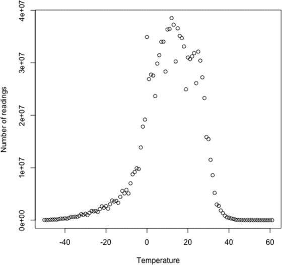
Figure 9-1. Temperature distribution for the weather dataset

This interface usually is not called directly by clients. Instead, the writePartitionFile() static method on InputSampler is used, which creates a sequence file to store the keys that define the partitions:

public static <K, V> void writePartitionFile(Job job, Sampler<K, V> sampler)

throws IOException, ClassNotFoundException, InterruptedException

The sequence file is used by TotalOrderPartitioner to create partitions for the sort job. Example 9-5 puts it all together.

Example 9-5. A MapReduce program for sorting a SequenceFile with IntWritable keys using the TotalOrderPartitioner to globally sort the data

public class SortByTemperatureUsingTotalOrderPartitioner extends Configured

implements Tool {

@Override

public int run(String[] args) throws Exception {

Job job = JobBuilder.parseInputAndOutput(this, getConf(), args);

if (job == null) {

return -1;

}

job.setInputFormatClass(SequenceFileInputFormat.class);

job.setOutputKeyClass(IntWritable.class);

job.setOutputFormatClass(SequenceFileOutputFormat.class);

SequenceFileOutputFormat.setCompressOutput(job, true);

SequenceFileOutputFormat.setOutputCompressorClass(job, GzipCodec.class);

SequenceFileOutputFormat.setOutputCompressionType(job,

CompressionType.BLOCK);

job.setPartitionerClass(TotalOrderPartitioner.class);

InputSampler.Sampler<IntWritable, Text> sampler =

new InputSampler.RandomSampler<IntWritable, Text>(0.1, 10000, 10);

InputSampler.writePartitionFile(job, sampler);

// Add to DistributedCache

Configuration conf = job.getConfiguration();

String partitionFile = TotalOrderPartitioner.getPartitionFile(conf);

URI partitionUri = new URI(partitionFile);

job.addCacheFile(partitionUri);

return job.waitForCompletion(true) ? 0 : 1;

}

public static void main(String[] args) throws Exception {

int exitCode = ToolRunner.run(

new SortByTemperatureUsingTotalOrderPartitioner(), args);

System.exit(exitCode);

}

}

We use a RandomSampler, which chooses keys with a uniform probability — here, 0.1. There are also parameters for the maximum number of samples to take and the maximum number of splits to sample (here, 10,000 and 10, respectively; these settings are the defaults whenInputSampler is run as an application), and the sampler stops when the first of these limits is met. Samplers run on the client, making it important to limit the number of splits that are downloaded so the sampler runs quickly. In practice, the time taken to run the sampler is a small fraction of the overall job time.

The InputSampler writes a partition file that we need to share with the tasks running on the cluster by adding it to the distributed cache (see Distributed Cache).

On one run, the sampler chose –5.6°C, 13.9°C, and 22.0°C as partition boundaries (for four partitions), which translates into more even partition sizes than the earlier choice:

Your input data determines the best sampler to use. For example, SplitSampler, which samples only the first n records in a split, is not so good for sorted data,^[64^] because it doesn’t select keys from throughout the split.

On the other hand, IntervalSampler chooses keys at regular intervals through the split and makes a better choice for sorted data. RandomSampler is a good general-purpose sampler. If none of these suits your application (and remember that the point of sampling is to produce partitions that are approximately equal in size), you can write your own implementation of the Sampler interface.

One of the nice properties of InputSampler and TotalOrderPartitioner is that you are free to choose the number of partitions — that is, the number of reducers. However, TotalOrderPartitioner will work only if the partition boundaries are distinct. One problem with choosing a high number is that you may get collisions if you have a small key space.

Here’s how we run it:

% hadoop jar hadoop-examples.jar SortByTemperatureUsingTotalOrderPartitioner \

-D mapreduce.job.reduces=30 input/ncdc/all-seq output-totalsort

The program produces 30 output partitions, each of which is internally sorted; in addition, for these partitions, all the keys in partition i are less than the keys in partition i + 1.

Secondary Sort

The MapReduce framework sorts the records by key before they reach the reducers. For any particular key, however, the values are not sorted. The order in which the values appear is not even stable from one run to the next, because they come from different map tasks, which may finish at different times from run to run. Generally speaking, most MapReduce programs are written so as not to depend on the order in which the values appear to the reduce function. However, it is possible to impose an order on the values by sorting and grouping the keys in a particular way.

To illustrate the idea, consider the MapReduce program for calculating the maximum temperature for each year. If we arranged for the values (temperatures) to be sorted in descending order, we wouldn’t have to iterate through them to find the maximum; instead, we could take the first for each year and ignore the rest. (This approach isn’t the most efficient way to solve this particular problem, but it illustrates how secondary sort works in general.)

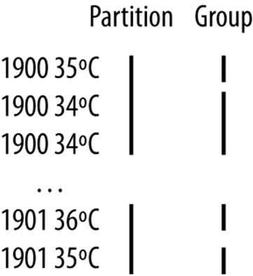
To achieve this, we change our keys to be composite: a combination of year and temperature. We want the sort order for keys to be by year (ascending) and then by temperature (descending):

1900 35°C

1900 34°C

1900 34°C

...

1901 36°C

1901 35°C

If all we did was change the key, this wouldn’t help, because then records for the same year would have different keys and therefore would not (in general) go to the same reducer. For example, (1900, 35°C) and (1900, 34°C) could go to different reducers. By setting a partitioner to partition by the year part of the key, we can guarantee that records for the same year go to the same reducer. This still isn’t enough to achieve our goal, however. A partitioner ensures only that one reducer receives all the records for a year; it doesn’t change the fact that the reducer groups by key within the partition:

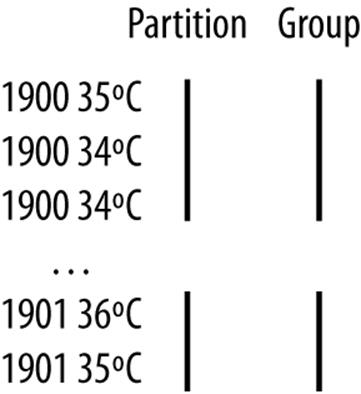
The final piece of the puzzle is the setting to control the grouping. If we group values in the reducer by the year part of the key, we will see all the records for the same year in one reduce group. And because they are sorted by temperature in descending order, the first is the maximum temperature:

To summarize, there is a recipe here to get the effect of sorting by value:

§ Make the key a composite of the natural key and the natural value.

§ The sort comparator should order by the composite key (i.e., the natural key and natural value).

§ The partitioner and grouping comparator for the composite key should consider only the natural key for partitioning and grouping.

Java code

Putting this all together results in the code in Example 9-6. This program uses the plain-text input again.

Example 9-6. Application to find the maximum temperature by sorting temperatures in the key

public class MaxTemperatureUsingSecondarySort

extends Configured implements Tool {

static class MaxTemperatureMapper

extends Mapper<LongWritable, Text, IntPair, NullWritable> {

private NcdcRecordParser parser = new NcdcRecordParser();

@Override

protected void map(LongWritable key, Text value,

Context context) throws IOException, InterruptedException {

parser.parse(value);

if (parser.isValidTemperature()) {

context.write(new IntPair(parser.getYearInt(),

parser.getAirTemperature()), NullWritable.get());

}

}

}

static class MaxTemperatureReducer

extends Reducer<IntPair, NullWritable, IntPair, NullWritable> {

@Override

protected void reduce(IntPair key, Iterable<NullWritable> values,

Context context) throws IOException, InterruptedException {

context.write(key, NullWritable.get());

}

}

public static class FirstPartitioner

extends Partitioner<IntPair, NullWritable> {

@Override

public int getPartition(IntPair key, NullWritable value, int numPartitions) {

// multiply by 127 to perform some mixing

return Math.abs(key.getFirst() * 127) % numPartitions;

}

}

public static class KeyComparator extends WritableComparator {

protected KeyComparator() {

super(IntPair.class, true);

}

@Override

public int compare(WritableComparable w1, WritableComparable w2) {

IntPair ip1 = (IntPair) w1;

IntPair ip2 = (IntPair) w2;

int cmp = IntPair.compare(ip1.getFirst(), ip2.getFirst());

if (cmp != 0) {

return cmp;

}

return -IntPair.compare(ip1.getSecond(), ip2.getSecond()); //reverse

}

}

public static class GroupComparator extends WritableComparator {

protected GroupComparator() {

super(IntPair.class, true);

}

@Override

public int compare(WritableComparable w1, WritableComparable w2) {

IntPair ip1 = (IntPair) w1;

IntPair ip2 = (IntPair) w2;

return IntPair.compare(ip1.getFirst(), ip2.getFirst());

}

}

@Override

public int run(String[] args) throws Exception {

Job job = JobBuilder.parseInputAndOutput(this, getConf(), args);

if (job == null) {

return -1;

}

job.setMapperClass(MaxTemperatureMapper.class);

job.setPartitionerClass(FirstPartitioner.class);

job.setSortComparatorClass(KeyComparator.class);

job.setGroupingComparatorClass(GroupComparator.class);

job.setReducerClass(MaxTemperatureReducer.class);

job.setOutputKeyClass(IntPair.class);

job.setOutputValueClass(NullWritable.class);

return job.waitForCompletion(true) ? 0 : 1;

}

public static void main(String[] args) throws Exception {

int exitCode = ToolRunner.run(new MaxTemperatureUsingSecondarySort(), args);

System.exit(exitCode);

}

}

In the mapper, we create a key representing the year and temperature, using an IntPair Writable implementation. (IntPair is like the TextPair class we developed in Implementing a Custom Writable.) We don’t need to carry any information in the value, because we can get the first (maximum) temperature in the reducer from the key, so we use a NullWritable. The reducer emits the first key, which, due to the secondary sorting, is an IntPair for the year and its maximum temperature. IntPair’s toString() method creates a tab-separated string, so the output is a set of tab-separated year-temperature pairs.

NOTE

Many applications need to access all the sorted values, not just the first value as we have provided here. To do this, you need to populate the value fields since in the reducer you can retrieve only the first key. This necessitates some unavoidable duplication of information between key and value.

We set the partitioner to partition by the first field of the key (the year) using a custom partitioner called FirstPartitioner. To sort keys by year (ascending) and temperature (descending), we use a custom sort comparator, using setSortComparatorClass(), that extracts the fields and performs the appropriate comparisons. Similarly, to group keys by year, we set a custom comparator, using setGroupingComparatorClass(), to extract the first field of the key for comparison.^[65^]

Running this program gives the maximum temperatures for each year:

% hadoop jar hadoop-examples.jar MaxTemperatureUsingSecondarySort \

input/ncdc/all output-secondarysort

% hadoop fs -cat output-secondarysort/part-* | sort | head

1901 317

1902 244

1903 289

1904 256

1905 283

1906 294

1907 283

1908 289

1909 278

1910 294

Streaming

To do a secondary sort in Streaming, we can take advantage of a couple of library classes that Hadoop provides. Here’s the driver that we can use to do a secondary sort:

% hadoop jar $HADOOP_HOME/share/hadoop/tools/lib/hadoop-streaming-*.jar \

-D stream.num.map.output.key.fields=2 \

-D mapreduce.partition.keypartitioner.options=-k1,1 \

-D mapreduce.job.output.key.comparator.class=\

org.apache.hadoop.mapred.lib.KeyFieldBasedComparator \

-D mapreduce.partition.keycomparator.options="-k1n -k2nr" \

-files secondary_sort_map.py,secondary_sort_reduce.py \

-input input/ncdc/all \

-output output-secondarysort-streaming \

-mapper ch09-mr-features/src/main/python/secondary_sort_map.py \

-partitioner org.apache.hadoop.mapred.lib.KeyFieldBasedPartitioner \

-reducer ch09-mr-features/src/main/python/secondary_sort_reduce.py

Our map function (Example 9-7) emits records with year and temperature fields. We want to treat the combination of both of these fields as the key, so we set stream.num.map.output.key.fields to 2. This means that values will be empty, just like in the Java case.

Example 9-7. Map function for secondary sort in Python

#!/usr/bin/env python

import re

import sys

for line insys.stdin:

val = line.strip()

(year, temp, q) = (val[15:19], int(val[87:92]), val[92:93])

if temp == 9999:

sys.stderr.write("reporter:counter:Temperature,Missing,1\n")

elif re.match("[01459]", q):

print "%s\t%s" % (year, temp)

However, we don’t want to partition by the entire key, so we use KeyFieldBasedPartitioner, which allows us to partition by a part of the key. The specification mapreduce.partition.keypartitioner.options configures the partitioner. The value -k1,1 instructs the partitioner to use only the first field of the key, where fields are assumed to be separated by a string defined by the mapreduce.map.output.key.field.separator property (a tab character by default).

Next, we want a comparator that sorts the year field in ascending order and the temperature field in descending order, so that the reduce function can simply return the first record in each group. Hadoop provides KeyFieldBasedComparator, which is ideal for this purpose. The comparison order is defined by a specification that is like the one used for GNU sort. It is set using the mapreduce.partition.keycomparator.options property. The value -k1n -k2nr used in this example means “sort by the first field in numerical order, then by the second field in reverse numerical order.” Like its partitioner cousin, KeyFieldBasedPartitioner, it uses the map output key separator to split a key into fields.

In the Java version, we had to set the grouping comparator; however, in Streaming, groups are not demarcated in any way, so in the reduce function we have to detect the group boundaries ourselves by looking for when the year changes (Example 9-8).

Example 9-8. Reduce function for secondary sort in Python

#!/usr/bin/env python

import sys

last_group = None

for line insys.stdin:

val = line.strip()

(year, temp) = val.split("\t")

group = year

if last_group != group:

print val

last_group = group

When we run the Streaming program, we get the same output as the Java version.

Finally, note that KeyFieldBasedPartitioner and KeyFieldBasedComparator are not confined to use in Streaming programs; they are applicable to Java MapReduce programs, too.

Joins

MapReduce can perform joins between large datasets, but writing the code to do joins from scratch is fairly involved. Rather than writing MapReduce programs, you might consider using a higher-level framework such as Pig, Hive, Cascading, Cruc, or Spark, in which join operations are a core part of the implementation.

Let’s briefly consider the problem we are trying to solve. We have two datasets — for example, the weather stations database and the weather records — and we want to reconcile the two. Let’s say we want to see each station’s history, with the station’s metadata inlined in each output row. This is illustrated in Figure 9-2.

How we implement the join depends on how large the datasets are and how they are partitioned. If one dataset is large (the weather records) but the other one is small enough to be distributed to each node in the cluster (as the station metadata is), the join can be effected by a MapReduce job that brings the records for each station together (a partial sort on station ID, for example). The mapper or reducer uses the smaller dataset to look up the station metadata for a station ID, so it can be written out with each record. See Side Data Distribution for a discussion of this approach, where we focus on the mechanics of distributing the data to nodes in the cluster.

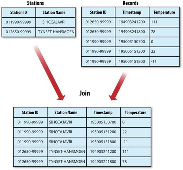
Figure 9-2. Inner join of two datasets

If the join is performed by the mapper it is called a map-side join, whereas if it is performed by the reducer it is called a reduce-side join.

If both datasets are too large for either to be copied to each node in the cluster, we can still join them using MapReduce with a map-side or reduce-side join, depending on how the data is structured. One common example of this case is a user database and a log of some user activity (such as access logs). For a popular service, it is not feasible to distribute the user database (or the logs) to all the MapReduce nodes.

Map-Side Joins

A map-side join between large inputs works by performing the join before the data reaches the map function. For this to work, though, the inputs to each map must be partitioned and sorted in a particular way. Each input dataset must be divided into the same number of partitions, and it must be sorted by the same key (the join key) in each source. All the records for a particular key must reside in the same partition. This may sound like a strict requirement (and it is), but it actually fits the description of the output of a MapReduce job.

A map-side join can be used to join the outputs of several jobs that had the same number of reducers, the same keys, and output files that are not splittable (by virtue of being smaller than an HDFS block or being gzip compressed, for example). In the context of the weather example, if we ran a partial sort on the stations file by station ID, and another identical sort on the records, again by station ID and with the same number of reducers, then the two outputs would satisfy the conditions for running a map-side join.

You use a CompositeInputFormat from the org.apache.hadoop.mapreduce.join package to run a map-side join. The input sources and join type (inner or outer) for CompositeInputFormat are configured through a join expression that is written according to a simple grammar. The package documentation has details and examples.

The org.apache.hadoop.examples.Join example is a general-purpose command-line program for running a map-side join, since it allows you to run a MapReduce job for any specified mapper and reducer over multiple inputs that are joined with a given join operation.

Reduce-Side Joins

A reduce-side join is more general than a map-side join, in that the input datasets don’t have to be structured in any particular way, but it is less efficient because both datasets have to go through the MapReduce shuffle. The basic idea is that the mapper tags each record with its source and uses the join key as the map output key, so that the records with the same key are brought together in the reducer. We use several ingredients to make this work in practice:

Multiple inputs

The input sources for the datasets generally have different formats, so it is very convenient to use the MultipleInputs class (see Multiple Inputs) to separate the logic for parsing and tagging each source.

Secondary sort

As described, the reducer will see the records from both sources that have the same key, but they are not guaranteed to be in any particular order. However, to perform the join, it is important to have the data from one source before that from the other. For the weather data join, the station record must be the first of the values seen for each key, so the reducer can fill in the weather records with the station name and emit them straightaway. Of course, it would be possible to receive the records in any order if we buffered them in memory, but this should be avoided because the number of records in any group may be very large and exceed the amount of memory available to the reducer.

We saw in Secondary Sort how to impose an order on the values for each key that the reducers see, so we use this technique here.

To tag each record, we use TextPair (discussed in Chapter 5) for the keys (to store the station ID) and the tag. The only requirement for the tag values is that they sort in such a way that the station records come before the weather records. This can be achieved by tagging station records as 0 and weather records as 1. The mapper classes to do this are shown in Examples 9-9 and 9-10.

Example 9-9. Mapper for tagging station records for a reduce-side join

public class JoinStationMapper

extends Mapper<LongWritable, Text, TextPair, Text> {

private NcdcStationMetadataParser parser = new NcdcStationMetadataParser();

@Override

protected void map(LongWritable key, Text value, Context context)

throws IOException, InterruptedException {

if (parser.parse(value)) {

context.write(new TextPair(parser.getStationId(), "0"),

new Text(parser.getStationName()));

}

}

}

Example 9-10. Mapper for tagging weather records for a reduce-side join

public class JoinRecordMapper

extends Mapper<LongWritable, Text, TextPair, Text> {

private NcdcRecordParser parser = new NcdcRecordParser();

@Override

protected void map(LongWritable key, Text value, Context context)

throws IOException, InterruptedException {

parser.parse(value);

context.write(new TextPair(parser.getStationId(), "1"), value);

}

}

The reducer knows that it will receive the station record first, so it extracts its name from the value and writes it out as a part of every output record (Example 9-11).

Example 9-11. Reducer for joining tagged station records with tagged weather records

public class JoinReducer extends Reducer<TextPair, Text, Text, Text> {

@Override

protected void reduce(TextPair key, Iterable<Text> values, Context context)

throws IOException, InterruptedException {

Iterator<Text> iter = values.iterator();

Text stationName = new Text(iter.next());

while (iter.hasNext()) {

Text record = iter.next();

Text outValue = new Text(stationName.toString() + "\t" + record.toString());

context.write(key.getFirst(), outValue);

}

}

}

The code assumes that every station ID in the weather records has exactly one matching record in the station dataset. If this were not the case, we would need to generalize the code to put the tag into the value objects, by using another TextPair. The reduce() method would then be able to tell which entries were station names and detect (and handle) missing or duplicate entries before processing the weather records.

WARNING

Because objects in the reducer’s values iterator are reused (for efficiency purposes), it is vital that the code makes a copy of the first Text object from the values iterator:

Text stationName = new Text(iter.next());

If the copy is not made, the stationName reference will refer to the value just read when it is turned into a string, which is a bug.

Tying the job together is the driver class, shown in Example 9-12. The essential point here is that we partition and group on the first part of the key, the station ID, which we do with a custom Partitioner (KeyPartitioner) and a custom group comparator, FirstComparator (fromTextPair).

Example 9-12. Application to join weather records with station names

public class JoinRecordWithStationName extends Configured implements Tool {

public static class KeyPartitioner extends Partitioner<TextPair, Text> {

@Override

public int getPartition(TextPair key, Text value, int numPartitions) {

return (key.getFirst().hashCode() & Integer.MAX_VALUE) % numPartitions;

}

}

@Override

public int run(String[] args) throws Exception {

if (args.length != 3) {

JobBuilder.printUsage(this, "<ncdc input> <station input> <output>");

return -1;

}

Job job = new Job(getConf(), "Join weather records with station names");

job.setJarByClass(getClass());

Path ncdcInputPath = new Path(args[0]);

Path stationInputPath = new Path(args[1]);

Path outputPath = new Path(args[2]);

MultipleInputs.addInputPath(job, ncdcInputPath,

TextInputFormat.class, JoinRecordMapper.class);

MultipleInputs.addInputPath(job, stationInputPath,

TextInputFormat.class, JoinStationMapper.class);

FileOutputFormat.setOutputPath(job, outputPath);

job.setPartitionerClass(KeyPartitioner.class);

job.setGroupingComparatorClass(TextPair.FirstComparator.class);

job.setMapOutputKeyClass(TextPair.class);

job.setReducerClass(JoinReducer.class);

job.setOutputKeyClass(Text.class);

return job.waitForCompletion(true) ? 0 : 1;

}

public static void main(String[] args) throws Exception {

int exitCode = ToolRunner.run(new JoinRecordWithStationName(), args);

System.exit(exitCode);

}

}

Running the program on the sample data yields the following output:

011990-99999 SIHCCAJAVRI 0067011990999991950051507004...

011990-99999 SIHCCAJAVRI 0043011990999991950051512004...

011990-99999 SIHCCAJAVRI 0043011990999991950051518004...

012650-99999 TYNSET-HANSMOEN 0043012650999991949032412004...

012650-99999 TYNSET-HANSMOEN 0043012650999991949032418004...

Side Data Distribution

Side data can be defined as extra read-only data needed by a job to process the main dataset. The challenge is to make side data available to all the map or reduce tasks (which are spread across the cluster) in a convenient and efficient fashion.

Using the Job Configuration

You can set arbitrary key-value pairs in the job configuration using the various setter methods on Configuration (or JobConf in the old MapReduce API). This is very useful when you need to pass a small piece of metadata to your tasks.

In the task, you can retrieve the data from the configuration returned by Context’s getConfiguration() method. (In the old API, it’s a little more involved: override the configure() method in the Mapper or Reducer and use a getter method on the JobConf object passed in to retrieve the data. It’s very common to store the data in an instance field so it can be used in the map() or reduce() method.)

Usually a primitive type is sufficient to encode your metadata, but for arbitrary objects you can either handle the serialization yourself (if you have an existing mechanism for turning objects to strings and back) or use Hadoop’s Stringifier class. The DefaultStringifier uses Hadoop’s serialization framework to serialize objects (see Serialization).

You shouldn’t use this mechanism for transferring more than a few kilobytes of data, because it can put pressure on the memory usage in MapReduce components. The job configuration is always read by the client, the application master, and the task JVM, and each time the configuration is read, all of its entries are read into memory, even if they are not used.

Distributed Cache

Rather than serializing side data in the job configuration, it is preferable to distribute datasets using Hadoop’s distributed cache mechanism. This provides a service for copying files and archives to the task nodes in time for the tasks to use them when they run. To save network bandwidth, files are normally copied to any particular node once per job.

Usage

For tools that use GenericOptionsParser (this includes many of the programs in this book; see GenericOptionsParser, Tool, and ToolRunner), you can specify the files to be distributed as a comma-separated list of URIs as the argument to the -files option. Files can be on the local filesystem, on HDFS, or on another Hadoop-readable filesystem (such as S3). If no scheme is supplied, then the files are assumed to be local. (This is true even when the default filesystem is not the local filesystem.)

You can also copy archive files (JAR files, ZIP files, tar files, and gzipped tar files) to your tasks using the -archives option; these are unarchived on the task node. The -libjars option will add JAR files to the classpath of the mapper and reducer tasks. This is useful if you haven’t bundled library JAR files in your job JAR file.

Let’s see how to use the distributed cache to share a metadata file for station names. The command we will run is:

% hadoop jar hadoop-examples.jar \

MaxTemperatureByStationNameUsingDistributedCacheFile \

-files input/ncdc/metadata/stations-fixed-width.txt input/ncdc/all output

This command will copy the local file stations-fixed-width.txt (no scheme is supplied, so the path is automatically interpreted as a local file) to the task nodes, so we can use it to look up station names. The listing for MaxTemperatureByStationNameUsingDistributedCacheFile appears inExample 9-13.

Example 9-13. Application to find the maximum temperature by station, showing station names from a lookup table passed as a distributed cache file

public class MaxTemperatureByStationNameUsingDistributedCacheFile

extends Configured implements Tool {

static class StationTemperatureMapper

extends Mapper<LongWritable, Text, Text, IntWritable> {

private NcdcRecordParser parser = new NcdcRecordParser();

@Override

protected void map(LongWritable key, Text value, Context context)

throws IOException, InterruptedException {

parser.parse(value);

if (parser.isValidTemperature()) {

context.write(new Text(parser.getStationId()),

new IntWritable(parser.getAirTemperature()));

}

}

}

static class MaxTemperatureReducerWithStationLookup

extends Reducer<Text, IntWritable, Text, IntWritable> {

private NcdcStationMetadata metadata;

@Override

protected void setup(Context context)

throws IOException, InterruptedException {

metadata = new NcdcStationMetadata();

metadata.initialize(new File("stations-fixed-width.txt"));

}

@Override

protected void reduce(Text key, Iterable<IntWritable> values,

Context context) throws IOException, InterruptedException {

String stationName = metadata.getStationName(key.toString());

int maxValue = Integer.MIN_VALUE;

for (IntWritable value : values) {

maxValue = Math.max(maxValue, value.get());

}

context.write(new Text(stationName), new IntWritable(maxValue));

}

}

@Override

public int run(String[] args) throws Exception {

Job job = JobBuilder.parseInputAndOutput(this, getConf(), args);

if (job == null) {

return -1;

}

job.setOutputKeyClass(Text.class);

job.setOutputValueClass(IntWritable.class);

job.setMapperClass(StationTemperatureMapper.class);

job.setCombinerClass(MaxTemperatureReducer.class);

job.setReducerClass(MaxTemperatureReducerWithStationLookup.class);

return job.waitForCompletion(true) ? 0 : 1;

}

public static void main(String[] args) throws Exception {

int exitCode = ToolRunner.run(

new MaxTemperatureByStationNameUsingDistributedCacheFile(), args);

System.exit(exitCode);

}

}

The program finds the maximum temperature by weather station, so the mapper (StationTemperatureMapper) simply emits (station ID, temperature) pairs. For the combiner, we reuse MaxTemperatureReducer (from Chapters 2 and 6) to pick the maximum temperature for any given group of map outputs on the map side. The reducer (MaxTemperatureReducerWithStationLookup) is different from the combiner, since in addition to finding the maximum temperature, it uses the cache file to look up the station name.

We use the reducer’s setup() method to retrieve the cache file using its original name, relative to the working directory of the task.

NOTE

You can use the distributed cache for copying files that do not fit in memory. Hadoop map files are very useful in this regard, since they serve as an on-disk lookup format (see MapFile). Because map files are collections of files with a defined directory structure, you should put them into an archive format (JAR, ZIP, tar, or gzipped tar) and add them to the cache using the -archivesoption.

Here’s a snippet of the output, showing some maximum temperatures for a few weather stations:

PEATS RIDGE WARATAH 372

STRATHALBYN RACECOU 410

SHEOAKS AWS 399

WANGARATTA AERO 409

MOOGARA 334

MACKAY AERO 331

How it works

When you launch a job, Hadoop copies the files specified by the -files, -archives, and -libjars options to the distributed filesystem (normally HDFS). Then, before a task is run, the node manager copies the files from the distributed filesystem to a local disk — the cache — so the task can access the files. The files are said to be localized at this point. From the task’s point of view, the files are just there, symbolically linked from the task’s working directory. In addition, files specified by -libjars are added to the task’s classpath before it is launched.

The node manager also maintains a reference count for the number of tasks using each file in the cache. Before the task has run, the file’s reference count is incremented by 1; then, after the task has run, the count is decreased by 1. Only when the file is not being used (when the count reaches zero) is it eligible for deletion. Files are deleted to make room for a new file when the node’s cache exceeds a certain size — 10 GB by default — using a least-recently used policy. The cache size may be changed by setting the configuration propertyyarn.nodemanager.localizer.cache.target-size-mb.

Although this design doesn’t guarantee that subsequent tasks from the same job running on the same node will find the file they need in the cache, it is very likely that they will: tasks from a job are usually scheduled to run at around the same time, so there isn’t the opportunity for enough other jobs to run to cause the original task’s file to be deleted from the cache.

The distributed cache API

Most applications don’t need to use the distributed cache API, because they can use the cache via GenericOptionsParser, as we saw in Example 9-13. However, if GenericOptionsParser is not being used, then the API in Job can be used to put objects into the distributed cache.^[66^] Here are the pertinent methods in Job:

public void addCacheFile(URI uri)

public void addCacheArchive(URI uri)

public void setCacheFiles(URI[] files)

public void setCacheArchives(URI[] archives)

public void addFileToClassPath(Path file)

public void addArchiveToClassPath(Path archive)

Recall that there are two types of objects that can be placed in the cache: files and archives. Files are left intact on the task node, whereas archives are unarchived on the task node. For each type of object, there are three methods: an addCacheXXXX() method to add the file or archive to the distributed cache, a setCacheXXXXs() method to set the entire list of files or archives to be added to the cache in a single call (replacing those set in any previous calls), and an addXXXXToClassPath() method to add the file or archive to the MapReduce task’s classpath. Table 9-7compares these API methods to the GenericOptionsParser options described in Table 6-1.

Table 9-7. Distributed cache API

NOTE

The URIs referenced in the add or set methods must be files in a shared filesystem that exist when the job is run. On the other hand, the filenames specified as a GenericOptionsParser option (e.g., -files) may refer to local files, in which case they get copied to the default shared filesystem (normally HDFS) on your behalf.

This is the key difference between using the Java API directly and using GenericOptionsParser: the Java API does not copy the file specified in the add or set method to the shared filesystem, whereas the GenericOptionsParser does.

Retrieving distributed cache files from the task works in the same way as before: you access the localized file directly by name, as we did in Example 9-13. This works because MapReduce will always create a symbolic link from the task’s working directory to every file or archive added to the distributed cache.^[67^] Archives are unarchived so you can access the files in them using the nested path.

MapReduce Library Classes

Hadoop comes with a library of mappers and reducers for commonly used functions. They are listed with brief descriptions in Table 9-8. For further information on how to use them, consult their Java documentation.

Table 9-8. MapReduce library classes

^[61^] One commonly used workaround for this problem — particularly in text-based Streaming applications — is to add an offset to eliminate all negative numbers and to left pad with zeros so all numbers are the same number of characters. However, see Streaming for another approach.

^[62^] See Sorting and merging SequenceFiles for how to do the same thing using the sort program example that comes with Hadoop.

^[63^] A better answer is to use Pig (Sorting Data), Hive (Sorting and Aggregating), Crunch, or Spark, all of which can sort with a single command.

^[64^] In some applications, it’s common for some of the input to already be sorted, or at least partially sorted. For example, the weather dataset is ordered by time, which may introduce certain biases, making the RandomSampler a safer choice.

^[65^] For simplicity, these custom comparators as shown are not optimized; see Implementing a RawComparator for speed for the steps we would need to take to make them faster.

^[66^] If you are using the old MapReduce API, the same methods can be found in org.apache.hadoop.filecache.DistributedCache.

^[67^] In Hadoop 1, localized files were not always symlinked, so it was sometimes necessary to retrieve localized file paths using methods on JobContext. This limitation was removed in Hadoop 2.