Hadoop: The Definitive Guide (2015)

Part IV. Related Projects

Chapter 15. Sqoop

Aaron Kimball

A great strength of the Hadoop platform is its ability to work with data in several different forms. HDFS can reliably store logs and other data from a plethora of sources, and MapReduce programs can parse diverse ad hoc data formats, extracting relevant information and combining multiple datasets into powerful results.

But to interact with data in storage repositories outside of HDFS, MapReduce programs need to use external APIs. Often, valuable data in an organization is stored in structured data stores such as relational database management systems (RDBMSs). Apache Sqoop is an open source tool that allows users to extract data from a structured data store into Hadoop for further processing. This processing can be done with MapReduce programs or other higher-level tools such as Hive. (It’s even possible to use Sqoop to move data from a database into HBase.) When the final results of an analytic pipeline are available, Sqoop can export these results back to the data store for consumption by other clients.

In this chapter, we’ll take a look at how Sqoop works and how you can use it in your data processing pipeline.

Getting Sqoop

Sqoop is available in a few places. The primary home of the project is the Apache Software Foundation. This repository contains all the Sqoop source code and documentation. Official releases are available at this site, as well as the source code for the version currently under development. The repository itself contains instructions for compiling the project. Alternatively, you can get Sqoop from a Hadoop vendor distribution.

If you download a release from Apache, it will be placed in a directory such as /home/yourname/sqoop-x.y.z/. We’ll call this directory $SQOOP_HOME. You can run Sqoop by running the executable script $SQOOP_HOME/bin/sqoop.

If you’ve installed a release from a vendor, the package will have placed Sqoop’s scripts in a standard location such as /usr/bin/sqoop. You can run Sqoop by simply typing sqoop at the command line. (Regardless of how you install Sqoop, we’ll refer to this script as just sqoop from here on.)

SQOOP 2

Sqoop 2 is a rewrite of Sqoop that addresses the architectural limitations of Sqoop 1. For example, Sqoop 1 is a command-line tool and does not provide a Java API, so it’s difficult to embed it in other programs. Also, in Sqoop 1 every connector has to know about every output format, so it is a lot of work to write new connectors. Sqoop 2 has a server component that runs jobs, as well as a range of clients: a command-line interface (CLI), a web UI, a REST API, and a Java API. Sqoop 2 also will be able to use alternative execution engines, such as Spark. Note that Sqoop 2’s CLI is not compatible with Sqoop 1’s CLI.

The Sqoop 1 release series is the current stable release series, and is what is used in this chapter. Sqoop 2 is under active development but does not yet have feature parity with Sqoop 1, so you should check that it can support your use case before using it in production.

Running Sqoop with no arguments does not do much of interest:

% sqoop

Try sqoop help for usage.

Sqoop is organized as a set of tools or commands. If you don’t select a tool, Sqoop does not know what to do. help is the name of one such tool; it can print out the list of available tools, like this:

% sqoop help

usage: sqoop COMMAND [ARGS]

Available commands:

codegen Generate code to interact with database records

create-hive-table Import a table definition into Hive

eval Evaluate a SQL statement and display the results

export Export an HDFS directory to a database table

help List available commands

import Import a table from a database to HDFS

import-all-tables Import tables from a database to HDFS

job Work with saved jobs

list-databases List available databases on a server

list-tables List available tables in a database

merge Merge results of incremental imports

metastore Run a standalone Sqoop metastore

version Display version information

See 'sqoop help COMMAND' for information on a specific command.

As it explains, the help tool can also provide specific usage instructions on a particular tool when you provide that tool’s name as an argument:

% sqoop help import

usage: sqoop import [GENERIC-ARGS] [TOOL-ARGS]

Common arguments:

--connect <jdbc-uri> Specify JDBC connect string

--driver <class-name> Manually specify JDBC driver class to use

--hadoop-home <dir> Override $HADOOP_HOME

--help Print usage instructions

-P Read password from console

--password <password> Set authentication password

--username <username> Set authentication username

--verbose Print more information while working

...

An alternate way of running a Sqoop tool is to use a tool-specific script. This script will be named sqoop-toolname (e.g., sqoop-help, sqoop-import, etc.). Running these scripts from the command line is identical to running sqoop help or sqoop import.

Sqoop Connectors

Sqoop has an extension framework that makes it possible to import data from — and export data to — any external storage system that has bulk data transfer capabilities. A Sqoop connector is a modular component that uses this framework to enable Sqoop imports and exports. Sqoop ships with connectors for working with a range of popular databases, including MySQL, PostgreSQL, Oracle, SQL Server, DB2, and Netezza. There is also a generic JDBC connector for connecting to any database that supports Java’s JDBC protocol. Sqoop provides optimized MySQL, PostgreSQL, Oracle, and Netezza connectors that use database-specific APIs to perform bulk transfers more efficiently (this is discussed more in Direct-Mode Imports).

As well as the built-in Sqoop connectors, various third-party connectors are available for data stores, ranging from enterprise data warehouses (such as Teradata) to NoSQL stores (such as Couchbase). These connectors must be downloaded separately and can be added to an existing Sqoop installation by following the instructions that come with the connector.

A Sample Import

After you install Sqoop, you can use it to import data to Hadoop. For the examples in this chapter, we’ll use MySQL, which is easy to use and available for a large number of platforms.

To install and configure MySQL, follow the online documentation. Chapter 2 (“Installing and Upgrading MySQL”) in particular should help. Users of Debian-based Linux systems (e.g., Ubuntu) can type sudo apt-get install mysql-client mysql-server. Red Hat users can typesudo yum install mysql mysql-server.

Now that MySQL is installed, let’s log in and create a database (Example 15-1).

Example 15-1. Creating a new MySQL database schema

% mysql -u root -p

Enter password:

Welcome to the MySQL monitor. Commands end with ; or \g.

Your MySQL connection id is 235

Server version: 5.6.21 MySQL Community Server (GPL)

Type 'help;' or '\h' for help. Type '\c' to clear the current input

statement.

mysql> CREATE DATABASE hadoopguide;

Query OK, 1 row affected (0.00 sec)

mysql> GRANT ALL PRIVILEGES ON hadoopguide.* TO ''@'localhost';

Query OK, 0 rows affected (0.00 sec)

mysql> quit;

Bye

The password prompt shown in this example asks for your root user password. This is likely the same as the password for the root shell login. If you are running Ubuntu or another variant of Linux where root cannot log in directly, enter the password you picked at MySQL installation time. (If you didn’t set a password, then just press Return.)

In this session, we created a new database schema called hadoopguide, which we’ll use throughout this chapter. We then allowed any local user to view and modify the contents of the hadoopguide schema, and closed our session.^[94^]

Now let’s log back into the database (do this as yourself this time, not as root) and create a table to import into HDFS (Example 15-2).

Example 15-2. Populating the database

% mysql hadoopguide

Welcome to the MySQL monitor. Commands end with ; or \g.

Your MySQL connection id is 257

Server version: 5.6.21 MySQL Community Server (GPL)

Type 'help;' or '\h' for help. Type '\c' to clear the current input statement.

mysql> CREATE TABLE widgets(id INT NOT NULL PRIMARY KEY AUTO_INCREMENT,

-> widget_name VARCHAR(64) NOT NULL,

-> price DECIMAL(10,2),

-> design_date DATE,

-> version INT,

-> design_comment VARCHAR(100));

Query OK, 0 rows affected (0.00 sec)

mysql> INSERT INTO widgets VALUES (NULL, 'sprocket', 0.25, '2010-02-10',

-> 1, 'Connects two gizmos');

Query OK, 1 row affected (0.00 sec)

mysql> INSERT INTO widgets VALUES (NULL, 'gizmo', 4.00, '2009-11-30', 4,

-> NULL);

Query OK, 1 row affected (0.00 sec)

mysql> INSERT INTO widgets VALUES (NULL, 'gadget', 99.99, '1983-08-13',

-> 13, 'Our flagship product');

Query OK, 1 row affected (0.00 sec)

mysql> quit;

In this listing, we created a new table called widgets. We’ll be using this fictional product database in further examples in this chapter. The widgets table contains several fields representing a variety of data types.

Before going any further, you need to download the JDBC driver JAR file for MySQL (Connector/J) and add it to Sqoop’s classpath, which is simply achieved by placing it in Sqoop’s lib directory.

Now let’s use Sqoop to import this table into HDFS:

% sqoop import --connect jdbc:mysql://localhost/hadoopguide \

> --table widgets -m 1

...

14/10/28 21:36:23 INFO tool.CodeGenTool: Beginning code generation

...

14/10/28 21:36:28 INFO mapreduce.Job: Running job: job_1413746845532_0008

14/10/28 21:36:35 INFO mapreduce.Job: Job job_1413746845532_0008 running in

uber mode : false

14/10/28 21:36:35 INFO mapreduce.Job: map 0% reduce 0%

14/10/28 21:36:41 INFO mapreduce.Job: map 100% reduce 0%

14/10/28 21:36:41 INFO mapreduce.Job: Job job_1413746845532_0008 completed

successfully

...

14/10/28 21:36:41 INFO mapreduce.ImportJobBase: Retrieved 3 records.

Sqoop’s import tool will run a MapReduce job that connects to the MySQL database and reads the table. By default, this will use four map tasks in parallel to speed up the import process. Each task will write its imported results to a different file, but all in a common directory. Because we knew that we had only three rows to import in this example, we specified that Sqoop should use a single map task (-m 1) so we get a single file in HDFS.

We can inspect this file’s contents like so:

% hadoop fs -cat widgets/part-m-00000

1,sprocket,0.25,2010-02-10,1,Connects two gizmos

2,gizmo,4.00,2009-11-30,4,null

3,gadget,99.99,1983-08-13,13,Our flagship product

NOTE

The connect string (jdbc:mysql://localhost/hadoopguide) shown in the example will read from a database on the local machine. If a distributed Hadoop cluster is being used, localhost should not be specified in the connect string, because map tasks not running on the same machine as the database will fail to connect. Even if Sqoop is run from the same host as the database sever, the full hostname should be specified.

By default, Sqoop will generate comma-delimited text files for our imported data. Delimiters can be specified explicitly, as well as field enclosing and escape characters, to allow the presence of delimiters in the field contents. The command-line arguments that specify delimiter characters, file formats, compression, and more fine-grained control of the import process are described in the Sqoop User Guide distributed with Sqoop,^[95^] as well as in the online help (sqoop help import, or man sqoop-import in CDH).

Text and Binary File Formats

Sqoop is capable of importing into a few different file formats. Text files (the default) offer a human-readable representation of data, platform independence, and the simplest structure. However, they cannot hold binary fields (such as database columns of type VARBINARY), and distinguishing between null values and String-based fields containing the value "null" can be problematic (although using the --null-string import option allows you to control the representation of null values).

To handle these conditions, Sqoop also supports SequenceFiles, Avro datafiles, and Parquet files. These binary formats provide the most precise representation possible of the imported data. They also allow data to be compressed while retaining MapReduce’s ability to process different sections of the same file in parallel. However, current versions of Sqoop cannot load Avro datafiles or SequenceFiles into Hive (although you can load Avro into Hive manually, and Parquet can be loaded directly into Hive by Sqoop). Another disadvantage of SequenceFiles is that they are Java specific, whereas Avro and Parquet files can be processed by a wide range of languages.

Generated Code

In addition to writing the contents of the database table to HDFS, Sqoop also provides you with a generated Java source file (widgets.java) written to the current local directory. (After running the sqoop import command shown earlier, you can see this file by running ls widgets.java.)

As you’ll learn in Imports: A Deeper Look, Sqoop can use generated code to handle the deserialization of table-specific data from the database source before writing it to HDFS.

The generated class (widgets) is capable of holding a single record retrieved from the imported table. It can manipulate such a record in MapReduce or store it in a SequenceFile in HDFS. (SequenceFiles written by Sqoop during the import process will store each imported row in the “value” element of the SequenceFile’s key-value pair format, using the generated class.)

It is likely that you don’t want to name your generated class widgets, since each instance of the class refers to only a single record. We can use a different Sqoop tool to generate source code without performing an import; this generated code will still examine the database table to determine the appropriate data types for each field:

% sqoop codegen --connect jdbc:mysql://localhost/hadoopguide \

> --table widgets --class-name Widget

The codegen tool simply generates code; it does not perform the full import. We specified that we’d like it to generate a class named Widget; this will be written to Widget.java. We also could have specified --class-name and other code-generation arguments during the import process we performed earlier. This tool can be used to regenerate code if you accidentally remove the source file, or generate code with different settings than were used during the import.

If you’re working with records imported to SequenceFiles, it is inevitable that you’ll need to use the generated classes (to deserialize data from the SequenceFile storage). You can work with text-file-based records without using generated code, but as we’ll see in Working with Imported Data, Sqoop’s generated code can handle some tedious aspects of data processing for you.

Additional Serialization Systems

Recent versions of Sqoop support Avro-based serialization and schema generation as well (see Chapter 12), allowing you to use Sqoop in your project without integrating with generated code.

Imports: A Deeper Look

As mentioned earlier, Sqoop imports a table from a database by running a MapReduce job that extracts rows from the table, and writes the records to HDFS. How does MapReduce read the rows? This section explains how Sqoop works under the hood.

At a high level, Figure 15-1 demonstrates how Sqoop interacts with both the database source and Hadoop. Like Hadoop itself, Sqoop is written in Java. Java provides an API called Java Database Connectivity, or JDBC, that allows applications to access data stored in an RDBMS as well as to inspect the nature of this data. Most database vendors provide a JDBC driver that implements the JDBC API and contains the necessary code to connect to their database servers.

NOTE

Based on the URL in the connect string used to access the database, Sqoop attempts to predict which driver it should load. You still need to download the JDBC driver itself and install it on your Sqoop client. For cases where Sqoop does not know which JDBC driver is appropriate, users can specify the JDBC driver explicitly with the --driver argument. This capability allows Sqoop to work with a wide variety of database platforms.

Before the import can start, Sqoop uses JDBC to examine the table it is to import. It retrieves a list of all the columns and their SQL data types. These SQL types (VARCHAR, INTEGER, etc.) can then be mapped to Java data types (String, Integer, etc.), which will hold the field values in MapReduce applications. Sqoop’s code generator will use this information to create a table-specific class to hold a record extracted from the table.

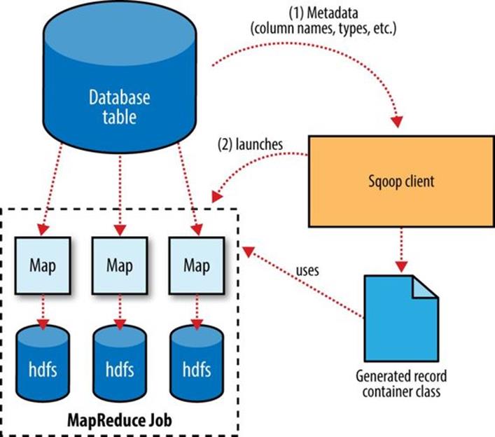
Figure 15-1. Sqoop’s import process

The Widget class from earlier, for example, contains the following methods that retrieve each column from an extracted record:

public Integer get_id();

public String get_widget_name();

public java.math.BigDecimal get_price();

public java.sql.Date get_design_date();

public Integer get_version();

public String get_design_comment();

More critical to the import system’s operation, though, are the serialization methods that form the DBWritable interface, which allow the Widget class to interact with JDBC:

public void readFields(ResultSet __dbResults) throws SQLException;

public void write(PreparedStatement __dbStmt) throws SQLException;

JDBC’s ResultSet interface provides a cursor that retrieves records from a query; the readFields() method here will populate the fields of the Widget object with the columns from one row of the ResultSet’s data. The write() method shown here allows Sqoop to insert new Widgetrows into a table, a process called exporting. Exports are discussed in Performing an Export.

The MapReduce job launched by Sqoop uses an InputFormat that can read sections of a table from a database via JDBC. The DataDrivenDBInputFormat provided with Hadoop partitions a query’s results over several map tasks.

Reading a table is typically done with a simple query such as:

SELECT col1,col2,col3,... FROM tableName

But often, better import performance can be gained by dividing this query across multiple nodes. This is done using a splitting column. Using metadata about the table, Sqoop will guess a good column to use for splitting the table (typically the primary key for the table, if one exists). The minimum and maximum values for the primary key column are retrieved, and then these are used in conjunction with a target number of tasks to determine the queries that each map task should issue.

For example, suppose the widgets table had 100,000 entries, with the id column containing values 0 through 99,999. When importing this table, Sqoop would determine that id is the primary key column for the table. When starting the MapReduce job, the DataDrivenDBInputFormatused to perform the import would issue a statement such as SELECT MIN(id), MAX(id) FROM widgets. These values would then be used to interpolate over the entire range of data. Assuming we specified that five map tasks should run in parallel (with -m 5), this would result in each map task executing queries such as SELECT id, widget_name, ... FROM widgets WHERE id >= 0 AND id < 20000, SELECT id, widget_name, ... FROM widgets WHERE id >= 20000 AND id < 40000, and so on.

The choice of splitting column is essential to parallelizing work efficiently. If the id column were not uniformly distributed (perhaps there are no widgets with IDs between 50,000 and 75,000), then some map tasks might have little or no work to perform, whereas others would have a great deal. Users can specify a particular splitting column when running an import job (via the --split-by argument), to tune the job to the data’s actual distribution. If an import job is run as a single (sequential) task with -m 1, this split process is not performed.

After generating the deserialization code and configuring the InputFormat, Sqoop sends the job to the MapReduce cluster. Map tasks execute the queries and deserialize rows from the ResultSet into instances of the generated class, which are either stored directly in SequenceFiles or transformed into delimited text before being written to HDFS.

Controlling the Import

Sqoop does not need to import an entire table at a time. For example, a subset of the table’s columns can be specified for import. Users can also specify a WHERE clause to include in queries via the --where argument, which bounds the rows of the table to import. For example, if widgets 0 through 99,999 were imported last month, but this month our vendor catalog included 1,000 new types of widget, an import could be configured with the clause WHERE id >= 100000; this will start an import job to retrieve all the new rows added to the source database since the previous import run. User-supplied WHERE clauses are applied before task splitting is performed, and are pushed down into the queries executed by each task.

For more control — to perform column transformations, for example — users can specify a --query argument.

Imports and Consistency

When importing data to HDFS, it is important that you ensure access to a consistent snapshot of the source data. (Map tasks reading from a database in parallel are running in separate processes. Thus, they cannot share a single database transaction.) The best way to do this is to ensure that any processes that update existing rows of a table are disabled during the import.

Incremental Imports

It’s common to run imports on a periodic basis so that the data in HDFS is kept synchronized with the data stored in the database. To do this, there needs to be some way of identifying the new data. Sqoop will import rows that have a column value (for the column specified with --check-column) that is greater than some specified value (set via --last-value).

The value specified as --last-value can be a row ID that is strictly increasing, such as an AUTO_INCREMENT primary key in MySQL. This is suitable for the case where new rows are added to the database table, but existing rows are not updated. This mode is called append mode, and is activated via --incremental append. Another option is time-based incremental imports (specified by --incremental lastmodified), which is appropriate when existing rows may be updated, and there is a column (the check column) that records the last modified time of the update.

At the end of an incremental import, Sqoop will print out the value to be specified as --last-value on the next import. This is useful when running incremental imports manually, but for running periodic imports it is better to use Sqoop’s saved job facility, which automatically stores the last value and uses it on the next job run. Type sqoop job --help for usage instructions for saved jobs.

Direct-Mode Imports

Sqoop’s architecture allows it to choose from multiple available strategies for performing an import. Most databases will use the DataDrivenDBInputFormat-based approach described earlier. Some databases, however, offer specific tools designed to extract data quickly. For example, MySQL’s mysqldump application can read from a table with greater throughput than a JDBC channel. The use of these external tools is referred to as direct mode in Sqoop’s documentation. Direct mode must be specifically enabled by the user (via the --direct argument), as it is not as general purpose as the JDBC approach. (For example, MySQL’s direct mode cannot handle large objects, such as CLOB or BLOB columns, and that’s why Sqoop needs to use a JDBC-specific API to load these columns into HDFS.)

For databases that provide such tools, Sqoop can use these to great effect. A direct-mode import from MySQL is usually much more efficient (in terms of map tasks and time required) than a comparable JDBC-based import. Sqoop will still launch multiple map tasks in parallel. These tasks will then spawn instances of the mysqldump program and read its output. Sqoop can also perform direct-mode imports from PostgreSQL, Oracle, and Netezza.

Even when direct mode is used to access the contents of a database, the metadata is still queried through JDBC.

Working with Imported Data

Once data has been imported to HDFS, it is ready for processing by custom MapReduce programs. Text-based imports can easily be used in scripts run with Hadoop Streaming or in MapReduce jobs run with the default TextInputFormat.

To use individual fields of an imported record, though, the field delimiters (and any escape/enclosing characters) must be parsed and the field values extracted and converted to the appropriate data types. For example, the ID of the “sprocket” widget is represented as the string "1" in the text file, but should be parsed into an Integer or int variable in Java. The generated table class provided by Sqoop can automate this process, allowing you to focus on the actual MapReduce job to run. Each autogenerated class has several overloaded methods named parse() that operate on the data represented as Text, CharSequence, char[], or other common types.

The MapReduce application called MaxWidgetId (available in the example code) will find the widget with the highest ID. The class can be compiled into a JAR file along with Widget.java using the Maven POM that comes with the example code. The JAR file is called sqoop-examples.jar, and is executed like so:

% HADOOP_CLASSPATH=$SQOOP_HOME/sqoop-version.jar hadoop jar \

> sqoop-examples.jar MaxWidgetId -libjars $SQOOP_HOME/sqoop-version.jar

This command line ensures that Sqoop is on the classpath locally (via $HADOOP_CLASSPATH) when running the MaxWidgetId.run() method, as well as when map tasks are running on the cluster (via the -libjars argument).

When run, the maxwidget path in HDFS will contain a file named part-r-00000 with the following expected result:

3,gadget,99.99,1983-08-13,13,Our flagship product

It is worth noting that in this example MapReduce program, a Widget object was emitted from the mapper to the reducer; the autogenerated Widget class implements the Writable interface provided by Hadoop, which allows the object to be sent via Hadoop’s serialization mechanism, as well as written to and read from SequenceFiles.

The MaxWidgetId example is built on the new MapReduce API. MapReduce applications that rely on Sqoop-generated code can be built on the new or old APIs, though some advanced features (such as working with large objects) are more convenient to use in the new API.

Avro-based imports can be processed using the APIs described in Avro MapReduce. With the Generic Avro mapping, the MapReduce program does not need to use schema-specific generated code (although this is an option too, by using Avro’s Specific compiler; Sqoop does not do the code generation in this case). The example code includes a program called MaxWidgetIdGenericAvro, which finds the widget with the highest ID and writes out the result in an Avro datafile.

Imported Data and Hive

As we’ll see in Chapter 17, for many types of analysis, using a system such as Hive to handle relational operations can dramatically ease the development of the analytic pipeline. Especially for data originally from a relational data source, using Hive makes a lot of sense. Hive and Sqoop together form a powerful toolchain for performing analysis.

Suppose we had another log of data in our system, coming from a web-based widget purchasing system. This might return logfiles containing a widget ID, a quantity, a shipping address, and an order date.

Here is a snippet from an example log of this type:

1,15,120 Any St.,Los Angeles,CA,90210,2010-08-01

3,4,120 Any St.,Los Angeles,CA,90210,2010-08-01

2,5,400 Some Pl.,Cupertino,CA,95014,2010-07-30

2,7,88 Mile Rd.,Manhattan,NY,10005,2010-07-18

By using Hadoop to analyze this purchase log, we can gain insight into our sales operation. By combining this data with the data extracted from our relational data source (the widgets table), we can do better. In this example session, we will compute which zip code is responsible for the most sales dollars, so we can better focus our sales team’s operations. Doing this requires data from both the sales log and the widgets table.

The table shown in the previous code snippet should be in a local file named sales.log for this to work.

First, let’s load the sales data into Hive:

hive> CREATE TABLE sales(widget_id INT, qty INT,

> street STRING, city STRING, state STRING,

> zip INT, sale_date STRING)

> ROW FORMAT DELIMITED FIELDS TERMINATED BY ',';

OK

Time taken: 5.248 seconds

hive> LOAD DATA LOCAL INPATH "ch15-sqoop/sales.log" INTO TABLE sales;

...

Loading data to table default.sales

Table default.sales stats: [numFiles=1, numRows=0, totalSize=189, rawDataSize=0]

OK

Time taken: 0.6 seconds

Sqoop can generate a Hive table based on a table from an existing relational data source. We’ve already imported the widgets data to HDFS, so we can generate the Hive table definition and then load in the HDFS-resident data:

% sqoop create-hive-table --connect jdbc:mysql://localhost/hadoopguide \

> --table widgets --fields-terminated-by ','

...

14/10/29 11:54:52 INFO hive.HiveImport: OK

14/10/29 11:54:52 INFO hive.HiveImport: Time taken: 1.098 seconds

14/10/29 11:54:52 INFO hive.HiveImport: Hive import complete.

% hive

hive> LOAD DATA INPATH "widgets" INTO TABLE widgets;

Loading data to table widgets

OK

Time taken: 3.265 seconds

When creating a Hive table definition with a specific already imported dataset in mind, we need to specify the delimiters used in that dataset. Otherwise, Sqoop will allow Hive to use its default delimiters (which are different from Sqoop’s default delimiters).

NOTE

Hive’s type system is less rich than that of most SQL systems. Many SQL types do not have direct analogues in Hive. When Sqoop generates a Hive table definition for an import, it uses the best Hive type available to hold a column’s values. This may result in a decrease in precision. When this occurs, Sqoop will provide you with a warning message such as this one:

14/10/29 11:54:43 WARN hive.TableDefWriter:

Column design_date had to be

cast to a less precise type in Hive

This three-step process of importing data to HDFS, creating the Hive table, and then loading the HDFS-resident data into Hive can be shortened to one step if you know that you want to import straight from a database directly into Hive. During an import, Sqoop can generate the Hive table definition and then load in the data. Had we not already performed the import, we could have executed this command, which creates the widgets table in Hive based on the copy in MySQL:

% sqoop import --connect jdbc:mysql://localhost/hadoopguide \

> --table widgets -m 1 --hive-import

NOTE

Running sqoop import with the --hive-import argument will load the data directly from the source database into Hive; it infers a Hive schema automatically based on the schema for the table in the source database. Using this, you can get started working with your data in Hive with only one command.

Regardless of which data import route we chose, we can now use the widgets dataset and the sales dataset together to calculate the most profitable zip code. Let’s do so, and also save the result of this query in another table for later:

hive> CREATE TABLE zip_profits

> AS

> SELECT SUM(w.price * s.qty) AS sales_vol, s.zip FROM SALES s

> JOIN widgets w ON (s.widget_id = w.id) GROUP BY s.zip;

...

Moving data to: hdfs://localhost/user/hive/warehouse/zip_profits

...

OK

hive> SELECT * FROM zip_profits ORDER BY sales_vol DESC;

...

OK

403.71 90210

28.0 10005

20.0 95014

Importing Large Objects

Most databases provide the capability to store large amounts of data in a single field. Depending on whether this data is textual or binary in nature, it is usually represented as a CLOB or BLOB column in the table. These “large objects” are often handled specially by the database itself. In particular, most tables are physically laid out on disk as in Figure 15-2. When scanning through rows to determine which rows match the criteria for a particular query, this typically involves reading all columns of each row from disk. If large objects were stored “inline” in this fashion, they would adversely affect the performance of such scans. Therefore, large objects are often stored externally from their rows, as in Figure 15-3. Accessing a large object often requires “opening” it through the reference contained in the row.

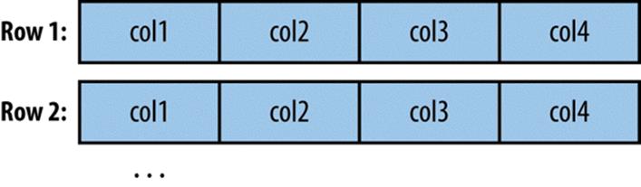
Figure 15-2. Database tables are typically physically represented as an array of rows, with all the columns in a row stored adjacent to one another

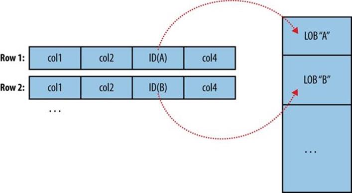
Figure 15-3. Large objects are usually held in a separate area of storage; the main row storage contains indirect references to the large objects

The difficulty of working with large objects in a database suggests that a system such as Hadoop, which is much better suited to storing and processing large, complex data objects, is an ideal repository for such information. Sqoop can extract large objects from tables and store them in HDFS for further processing.

As in a database, MapReduce typically materializes every record before passing it along to the mapper. If individual records are truly large, this can be very inefficient.

As shown earlier, records imported by Sqoop are laid out on disk in a fashion very similar to a database’s internal structure: an array of records with all fields of a record concatenated together. When running a MapReduce program over imported records, each map task must fully materialize all fields of each record in its input split. If the contents of a large object field are relevant only for a small subset of the total number of records used as input to a MapReduce program, it would be inefficient to fully materialize all these records. Furthermore, depending on the size of the large object, full materialization in memory may be impossible.

To overcome these difficulties, Sqoop will store imported large objects in a separate file called a LobFile, if they are larger than a threshold size of 16 MB (configurable via the sqoop.inline.lob.length.max setting, in bytes). The LobFile format can store individual records of very large size (a 64-bit address space is used). Each record in a LobFile holds a single large object. The LobFile format allows clients to hold a reference to a record without accessing the record contents. When records are accessed, this is done through a java.io.InputStream (for binary objects) or java.io.Reader (for character-based objects).

When a record is imported, the “normal” fields will be materialized together in a text file, along with a reference to the LobFile where a CLOB or BLOB column is stored. For example, suppose our widgets table contained a BLOB field named schematic holding the actual schematic diagram for each widget.

An imported record might then look like:

2,gizmo,4.00,2009-11-30,4,null,externalLob(lf,lobfile0,100,5011714)

The externalLob(...) text is a reference to an externally stored large object, stored in LobFile format (lf) in a file named lobfile0, with the specified byte offset and length inside that file.

When working with this record, the Widget.get_schematic() method would return an object of type BlobRef referencing the schematic column, but not actually containing its contents. The BlobRef.getDataStream() method actually opens the LobFile and returns an InputStream, allowing you to access the schematic field’s contents.

When running a MapReduce job processing many Widget records, you might need to access the schematic fields of only a handful of records. This system allows you to incur the I/O costs of accessing only the required large object entries — a big savings, as individual schematics may be several megabytes or more of data.

The BlobRef and ClobRef classes cache references to underlying LobFiles within a map task. If you do access the schematic fields of several sequentially ordered records, they will take advantage of the existing file pointer’s alignment on the next record body.

Performing an Export

In Sqoop, an import refers to the movement of data from a database system into HDFS. By contrast, an export uses HDFS as the source of data and a remote database as the destination. In the previous sections, we imported some data and then performed some analysis using Hive. We can export the results of this analysis to a database for consumption by other tools.

Before exporting a table from HDFS to a database, we must prepare the database to receive the data by creating the target table. Although Sqoop can infer which Java types are appropriate to hold SQL data types, this translation does not work in both directions (for example, there are several possible SQL column definitions that can hold data in a Java String; this could be CHAR(64), VARCHAR(200), or something else entirely). Consequently, you must determine which types are most appropriate.

We are going to export the zip_profits table from Hive. We need to create a table in MySQL that has target columns in the same order, with the appropriate SQL types:

% mysql hadoopguide

mysql> CREATE TABLE sales_by_zip (volume DECIMAL(8,2), zip INTEGER);

Query OK, 0 rows affected (0.01 sec)

Then we run the export command:

% sqoop export --connect jdbc:mysql://localhost/hadoopguide -m 1 \

> --table sales_by_zip --export-dir /user/hive/warehouse/zip_profits \

> --input-fields-terminated-by '\0001'

...

14/10/29 12:05:08 INFO mapreduce.ExportJobBase: Transferred 176 bytes in 13.5373

seconds (13.0011 bytes/sec)

14/10/29 12:05:08 INFO mapreduce.ExportJobBase: Exported 3 records.

Finally, we can verify that the export worked by checking MySQL:

% mysql hadoopguide -e 'SELECT * FROM sales_by_zip'

+--------+-------+

| volume | zip |

+--------+-------+

| 28.00 | 10005 |

| 403.71 | 90210 |

| 20.00 | 95014 |

+--------+-------+

When we created the zip_profits table in Hive, we did not specify any delimiters. So Hive used its default delimiters: a Ctrl-A character (Unicode 0x0001) between fields and a newline at the end of each record. When we used Hive to access the contents of this table (in a SELECTstatement), Hive converted this to a tab-delimited representation for display on the console. But when reading the tables directly from files, we need to tell Sqoop which delimiters to use. Sqoop assumes records are newline-delimited by default, but needs to be told about the Ctrl-A field delimiters. The --input-fields-terminated-by argument to sqoop export specified this information. Sqoop supports several escape sequences, which start with a backslash (\) character, when specifying delimiters.

In the example syntax, the escape sequence is enclosed in single quotes to ensure that the shell processes it literally. Without the quotes, the leading backslash itself may need to be escaped (e.g., --input-fields-terminated-by \\0001). The escape sequences supported by Sqoop are listed in Table 15-1.

Table 15-1. Escape sequences that can be used to specify nonprintable characters as field and record delimiters in Sqoop

Exports: A Deeper Look

The Sqoop performs exports is very similar in nature to how Sqoop performs imports (see Figure 15-4). Before performing the export, Sqoop picks a strategy based on the database connect string. For most systems, Sqoop uses JDBC. Sqoop then generates a Java class based on the target table definition. This generated class has the ability to parse records from text files and insert values of the appropriate types into a table (in addition to the ability to read the columns from a ResultSet). A MapReduce job is then launched that reads the source datafiles from HDFS, parses the records using the generated class, and executes the chosen export strategy.

The JDBC-based export strategy builds up batch INSERT statements that will each add multiple records to the target table. Inserting many records per statement performs much better than executing many single-row INSERT statements on most database systems. Separate threads are used to read from HDFS and communicate with the database, to ensure that I/O operations involving different systems are overlapped as much as possible.

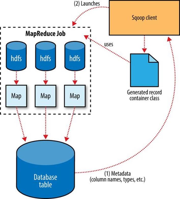
Figure 15-4. Exports are performed in parallel using MapReduce

For MySQL, Sqoop can employ a direct-mode strategy using mysqlimport. Each map task spawns a mysqlimport process that it communicates with via a named FIFO file on the local filesystem. Data is then streamed into mysqlimport via the FIFO channel, and from there into the database.

Whereas most MapReduce jobs reading from HDFS pick the degree of parallelism (number of map tasks) based on the number and size of the files to process, Sqoop’s export system allows users explicit control over the number of tasks. The performance of the export can be affected by the number of parallel writers to the database, so Sqoop uses the CombineFileInputFormat class to group the input files into a smaller number of map tasks.

Exports and Transactionality

Due to the parallel nature of the process, often an export is not an atomic operation. Sqoop will spawn multiple tasks to export slices of the data in parallel. These tasks can complete at different times, meaning that even though transactions are used inside tasks, results from one task may be visible before the results of another task. Moreover, databases often use fixed-size buffers to store transactions. As a result, one transaction cannot necessarily contain the entire set of operations performed by a task. Sqoop commits results every few thousand rows, to ensure that it does not run out of memory. These intermediate results are visible while the export continues. Applications that will use the results of an export should not be started until the export process is complete, or they may see partial results.

To solve this problem, Sqoop can export to a temporary staging table and then, at the end of the job — if the export has succeeded — move the staged data into the destination table in a single transaction. You can specify a staging table with the --staging-table option. The staging table must already exist and have the same schema as the destination. It must also be empty, unless the --clear-staging-table option is also supplied.

NOTE

Using a staging table is slower, since the data must be written twice: first to the staging table, then to the destination table. The export process also uses more space while it is running, since there are two copies of the data while the staged data is being copied to the destination.

Exports and SequenceFiles

The example export reads source data from a Hive table, which is stored in HDFS as a delimited text file. Sqoop can also export delimited text files that were not Hive tables. For example, it can export text files that are the output of a MapReduce job.

Sqoop can export records stored in SequenceFiles to an output table too, although some restrictions apply. A SequenceFile cannot contain arbitrary record types. Sqoop’s export tool will read objects from SequenceFiles and send them directly to the OutputCollector, which passes the objects to the database export OutputFormat. To work with Sqoop, the record must be stored in the “value” portion of the SequenceFile’s key-value pair format and must subclass the org.apache.sqoop.lib.SqoopRecord abstract class (as is done by all classes generated by Sqoop).

If you use the codegen tool (sqoop-codegen) to generate a SqoopRecord implementation for a record based on your export target table, you can write a MapReduce program that populates instances of this class and writes them to SequenceFiles. sqoop-export can then export theseSequenceFiles to the table. Another means by which data may be in SqoopRecord instances in SequenceFiles is if data is imported from a database table to HDFS and modified in some fashion, and then the results are stored in SequenceFiles holding records of the same data type.

In this case, Sqoop should reuse the existing class definition to read data from SequenceFiles, rather than generating a new (temporary) record container class to perform the export, as is done when converting text-based records to database rows. You can suppress code generation and instead use an existing record class and JAR by providing the --class-name and --jar-file arguments to Sqoop. Sqoop will use the specified class, loaded from the specified JAR, when exporting records.

In the following example, we reimport the widgets table as SequenceFiles, and then export it back to the database in a different table:

% sqoop import --connect jdbc:mysql://localhost/hadoopguide \

> --table widgets -m 1 --class-name WidgetHolder --as-sequencefile \

> --target-dir widget_sequence_files --bindir .

...

14/10/29 12:25:03 INFO mapreduce.ImportJobBase: Retrieved 3 records.

% mysql hadoopguide

mysql> CREATE TABLE widgets2(id INT, widget_name VARCHAR(100),

-> price DOUBLE, designed DATE, version INT, notes VARCHAR(200));

Query OK, 0 rows affected (0.03 sec)

mysql> exit;

% sqoop export --connect jdbc:mysql://localhost/hadoopguide \

> --table widgets2 -m 1 --class-name WidgetHolder \

> --jar-file WidgetHolder.jar --export-dir widget_sequence_files

...

14/10/29 12:28:17 INFO mapreduce.ExportJobBase: Exported 3 records.

During the import, we specified the SequenceFile format and indicated that we wanted the JAR file to be placed in the current directory (with --bindir) so we can reuse it. Otherwise, it would be placed in a temporary directory. We then created a destination table for the export, which had a slightly different schema (albeit one that is compatible with the original data). Finally, we ran an export that used the existing generated code to read the records from the SequenceFile and write them to the database.

Further Reading

For more information on using Sqoop, consult the Apache Sqoop Cookbook by Kathleen Ting and Jarek Jarcec Cecho (O’Reilly, 2013).

^[94^] Of course, in a production deployment we’d need to be much more careful about access control, but this serves for demonstration purposes. The grant privilege shown in the example also assumes you’re running a pseudodistributed Hadoop instance. If you’re working with a distributed Hadoop cluster, you’d need to enable remote access by at least one user, whose account would be used to perform imports and exports via Sqoop.

^[95^] Available from the Apache Software Foundation website.