Hadoop: The Definitive Guide (2015)
Part IV. Related Projects
Chapter 20. HBase
Jonathan Gray
Michael Stack
HBasics
HBase is a distributed column-oriented database built on top of HDFS. HBase is the Hadoop application to use when you require real-time read/write random access to very large datasets.
Although there are countless strategies and implementations for database storage and retrieval, most solutions — especially those of the relational variety — are not built with very large scale and distribution in mind. Many vendors offer replication and partitioning solutions to grow the database beyond the confines of a single node, but these add-ons are generally an afterthought and are complicated to install and maintain. They also severely compromise the RDBMS feature set. Joins, complex queries, triggers, views, and foreign-key constraints become prohibitively expensive to run on a scaled RDBMS, or do not work at all.
HBase approaches the scaling problem from the opposite direction. It is built from the ground up to scale linearly just by adding nodes. HBase is not relational and does not support SQL,[136] but given the proper problem space, it is able to do what an RDBMS cannot: host very large, sparsely populated tables on clusters made from commodity hardware.
The canonical HBase use case is the webtable, a table of crawled web pages and their attributes (such as language and MIME type) keyed by the web page URL. The webtable is large, with row counts that run into the billions. Batch analytic and parsing MapReduce jobs are continuously run against the webtable, deriving statistics and adding new columns of verified MIME-type and parsed-text content for later indexing by a search engine. Concurrently, the table is randomly accessed by crawlers running at various rates and updating random rows while random web pages are served in real time as users click on a website’s cached-page feature.
Backdrop
The HBase project was started toward the end of 2006 by Chad Walters and Jim Kellerman at Powerset. It was modeled after Google’s Bigtable, which had just been published.[137] In February 2007, Mike Cafarella made a code drop of a mostly working system that Jim Kellerman then carried forward.
The first HBase release was bundled as part of Hadoop 0.15.0 in October 2007. In May 2010, HBase graduated from a Hadoop subproject to become an Apache Top Level Project. Today, HBase is a mature technology used in production across a wide range of industries.
Concepts
In this section, we provide a quick overview of core HBase concepts. At a minimum, a passing familiarity will ease the digestion of all that follows.
Whirlwind Tour of the Data Model
Applications store data in labeled tables. Tables are made of rows and columns. Table cells — the intersection of row and column coordinates — are versioned. By default, their version is a timestamp auto-assigned by HBase at the time of cell insertion. A cell’s content is an uninterpreted array of bytes. An example HBase table for storing photos is shown in Figure 20-1.
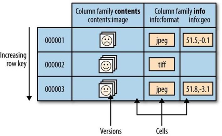
Figure 20-1. The HBase data model, illustrated for a table storing photos
Table row keys are also byte arrays, so theoretically anything can serve as a row key, from strings to binary representations of long or even serialized data structures. Table rows are sorted by row key, aka the table’s primary key. The sort is byte-ordered. All table accesses are via the primary key.[138]
Row columns are grouped into column families. All column family members have a common prefix, so, for example, the columns info:format and info:geo are both members of the info column family, whereas contents:image belongs to the contents family. The column family prefix must be composed of printable characters. The qualifying tail, the column family qualifier, can be made of any arbitrary bytes. The column family and the qualifier are always separated by a colon character (:).
A table’s column families must be specified up front as part of the table schema definition, but new column family members can be added on demand. For example, a new column info:camera can be offered by a client as part of an update, and its value persisted, as long as the column family info already exists on the table.
Physically, all column family members are stored together on the filesystem. So although earlier we described HBase as a column-oriented store, it would be more accurate if it were described as a column-family-oriented store. Because tuning and storage specifications are done at the column family level, it is advised that all column family members have the same general access pattern and size characteristics. For the photos table, the image data, which is large (megabytes), is stored in a separate column family from the metadata, which is much smaller in size (kilobytes).
In synopsis, HBase tables are like those in an RDBMS, only cells are versioned, rows are sorted, and columns can be added on the fly by the client as long as the column family they belong to preexists.
Regions
Tables are automatically partitioned horizontally by HBase into regions. Each region comprises a subset of a table’s rows. A region is denoted by the table it belongs to, its first row (inclusive), and its last row (exclusive). Initially, a table comprises a single region, but as the region grows it eventually crosses a configurable size threshold, at which point it splits at a row boundary into two new regions of approximately equal size. Until this first split happens, all loading will be against the single server hosting the original region. As the table grows, the number of its regions grows. Regions are the units that get distributed over an HBase cluster. In this way, a table that is too big for any one server can be carried by a cluster of servers, with each node hosting a subset of the table’s total regions. This is also the means by which the loading on a table gets distributed. The online set of sorted regions comprises the table’s total content.
Locking
Row updates are atomic, no matter how many row columns constitute the row-level transaction. This keeps the locking model simple.
Implementation
Just as HDFS and YARN are built of clients, workers, and a coordinating master — the namenode and datanodes in HDFS and resource manager and node managers in YARN — so is HBase made up of an HBase master node orchestrating a cluster of one or more regionserverworkers (see Figure 20-2). The HBase master is responsible for bootstrapping a virgin install, for assigning regions to registered regionservers, and for recovering regionserver failures. The master node is lightly loaded. The regionservers carry zero or more regions and field client read/write requests. They also manage region splits, informing the HBase master about the new daughter regions so it can manage the offlining of parent regions and assignment of the replacement daughters.
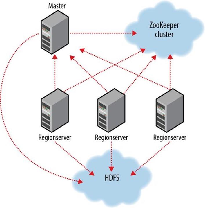
Figure 20-2. HBase cluster members
HBase depends on ZooKeeper (Chapter 21), and by default it manages a ZooKeeper instance as the authority on cluster state, although it can be configured to use an existing ZooKeeper cluster instead. The ZooKeeper ensemble hosts vitals such as the location of the hbase:metacatalog table and the address of the current cluster master. Assignment of regions is mediated via ZooKeeper in case participating servers crash mid-assignment. Hosting the assignment transaction state in ZooKeeper makes it so recovery can pick up on the assignment where the crashed server left off. At a minimum, when bootstrapping a client connection to an HBase cluster, the client must be passed the location of the ZooKeeper ensemble. Thereafter, the client navigates the ZooKeeper hierarchy to learn cluster attributes such as server locations.
Regionserver worker nodes are listed in the HBase conf/regionservers file, as you would list datanodes and node managers in the Hadoop etc/hadoop/slaves file. Start and stop scripts are like those in Hadoop and use the same SSH-based mechanism for running remote commands. A cluster’s site-specific configuration is done in the HBase conf/hbase-site.xml and conf/hbase-env.sh files, which have the same format as their equivalents in the Hadoop parent project (see Chapter 10).
NOTE
Where there is commonality to be found, whether in a service or type, HBase typically directly uses or subclasses the parent Hadoop implementation. When this is not possible, HBase will follow the Hadoop model where it can. For example, HBase uses the Hadoop configuration system, so configuration files have the same format. What this means for you, the user, is that you can leverage any Hadoop familiarity in your exploration of HBase. HBase deviates from this rule only when adding its specializations.
HBase persists data via the Hadoop filesystem API. Most people using HBase run it on HDFS for storage, though by default, and unless told otherwise, HBase writes to the local filesystem. The local filesystem is fine for experimenting with your initial HBase install, but thereafter, the first configuration made in an HBase cluster usually involves pointing HBase at the HDFS cluster it should use.
HBase in operation
Internally, HBase keeps a special catalog table named hbase:meta, within which it maintains the current list, state, and locations of all user-space regions afloat on the cluster. Entries in hbase:meta are keyed by region name, where a region name is made up of the name of the table the region belongs to, the region’s start row, its time of creation, and finally, an MD5 hash of all of these (i.e., a hash of table name, start row, and creation timestamp). Here is an example region name for a region in the table TestTable whose start row is xyz:
TestTable,xyz,1279729913622.1b6e176fb8d8aa88fd4ab6bc80247ece.
Commas delimit the table name, start row, and timestamp. The MD5 hash is surrounded by a leading and trailing period.
As noted previously, row keys are sorted, so finding the region that hosts a particular row is a matter of a lookup to find the largest entry whose key is less than or equal to that of the requested row key. As regions transition — are split, disabled, enabled, deleted, or redeployed by the region load balancer, or redeployed due to a regionserver crash — the catalog table is updated so the state of all regions on the cluster is kept current.
Fresh clients connect to the ZooKeeper cluster first to learn the location of hbase:meta. The client then does a lookup against the appropriate hbase:meta region to figure out the hosting user-space region and its location. Thereafter, the client interacts directly with the hosting regionserver.
To save on having to make three round-trips per row operation, clients cache all they learn while doing lookups for hbase:meta. They cache locations as well as user-space region start and stop rows, so they can figure out hosting regions themselves without having to go back to thehbase:meta table. Clients continue to use the cached entries as they work, until there is a fault. When this happens — i.e., when the region has moved — the client consults the hbase:meta table again to learn the new location. If the consulted hbase:meta region has moved, then ZooKeeper is reconsulted.
Writes arriving at a regionserver are first appended to a commit log and then added to an in-memory memstore. When a memstore fills, its content is flushed to the filesystem.
The commit log is hosted on HDFS, so it remains available through a regionserver crash. When the master notices that a regionserver is no longer reachable, usually because the server’s znode has expired in ZooKeeper, it splits the dead regionserver’s commit log by region. On reassignment and before they reopen for business, regions that were on the dead regionserver will pick up their just-split files of not-yet-persisted edits and replay them to bring themselves up to date with the state they had just before the failure.
When reading, the region’s memstore is consulted first. If sufficient versions are found reading memstore alone, the query completes there. Otherwise, flush files are consulted in order, from newest to oldest, either until versions sufficient to satisfy the query are found or until we run out of flush files.
A background process compacts flush files once their number has exceeded a threshold, rewriting many files as one, because the fewer files a read consults, the more performant it will be. On compaction, the process cleans out versions beyond the schema-configured maximum and removes deleted and expired cells. A separate process running in the regionserver monitors flush file sizes, splitting the region when they grow in excess of the configured maximum.
Installation
Download a stable release from an Apache Download Mirror and unpack it on your local filesystem. For example:
% tar xzf hbase-x.y.z.tar.gz
As with Hadoop, you first need to tell HBase where Java is located on your system. If you have the JAVA_HOME environment variable set to point to a suitable Java installation, then that will be used, and you don’t have to configure anything further. Otherwise, you can set the Java installation that HBase uses by editing HBase’s conf/hbase-env.sh file and specifying the JAVA_HOME variable (see Appendix A for some examples).
For convenience, add the HBase binary directory to your command-line path. For example:
% export HBASE_HOME=~/sw/hbase-x.y.z
% export PATH=$PATH:$HBASE_HOME/bin
To get the list of HBase options, use the following:
% hbase
Options:
--config DIR Configuration direction to use. Default: ./conf
--hosts HOSTS Override the list in 'regionservers' file
Commands:
Some commands take arguments. Pass no args or -h for usage.
shell Run the HBase shell
hbck Run the hbase 'fsck' tool
hlog Write-ahead-log analyzer
hfile Store file analyzer
zkcli Run the ZooKeeper shell
upgrade Upgrade hbase
master Run an HBase HMaster node
regionserver Run an HBase HRegionServer node
zookeeper Run a Zookeeper server
rest Run an HBase REST server
thrift Run the HBase Thrift server
thrift2 Run the HBase Thrift2 server
clean Run the HBase clean up script
classpath Dump hbase CLASSPATH
mapredcp Dump CLASSPATH entries required by mapreduce
pe Run PerformanceEvaluation
ltt Run LoadTestTool
version Print the version
CLASSNAME Run the class named CLASSNAME
Test Drive
To start a standalone instance of HBase that uses a temporary directory on the local filesystem for persistence, use this:
% start-hbase.sh
By default, HBase writes to /${java.io.tmpdir}/hbase-${user.name}. ${java.io.tmpdir} usually maps to /tmp, but you should configure HBase to use a more permanent location by setting hbase.tmp.dir in hbase-site.xml. In standalone mode, the HBase master, the regionserver, and aZooKeeper instance are all run in the same JVM.
To administer your HBase instance, launch the HBase shell as follows:
% hbase shell
HBase Shell; enter 'help<RETURN>' for list of supported commands.
Type "exit<RETURN>" to leave the HBase Shell
Version 0.98.7-hadoop2, r800c23e2207aa3f9bddb7e9514d8340bcfb89277, Wed Oct 8
15:58:11 PDT 2014
hbase(main):001:0>
This will bring up a JRuby IRB interpreter that has had some HBase-specific commands added to it. Type help and then press Return to see the list of shell commands grouped into categories. Type help "COMMAND_GROUP" for help by category or help "COMMAND" for help on a specific command and example usage. Commands use Ruby formatting to specify lists and dictionaries. See the end of the main help screen for a quick tutorial.
Now let’s create a simple table, add some data, and then clean up.
To create a table, you must name your table and define its schema. A table’s schema comprises table attributes and the list of table column families. Column families themselves have attributes that you in turn set at schema definition time. Examples of column family attributes include whether the family content should be compressed on the filesystem and how many versions of a cell to keep. Schemas can be edited later by offlining the table using the shell disable command, making the necessary alterations using alter, then putting the table back online withenable.
To create a table named test with a single column family named data using defaults for table and column family attributes, enter:
hbase(main):001:0> create 'test', 'data'
0 row(s) in 0.9810 seconds
TIP
If the previous command does not complete successfully, and the shell displays an error and a stack trace, your install was not successful. Check the master logs under the HBase logs directory — the default location for the logs directory is ${HBASE_HOME}/logs — for a clue as to where things went awry.
See the help output for examples of adding table and column family attributes when specifying a schema.
To prove the new table was created successfully, run the list command. This will output all tables in user space:
hbase(main):002:0> list
TABLE
test
1 row(s) in 0.0260 seconds
To insert data into three different rows and columns in the data column family, get the first row, and then list the table content, do the following:
hbase(main):003:0> put 'test', 'row1', 'data:1', 'value1'
hbase(main):004:0> put 'test', 'row2', 'data:2', 'value2'
hbase(main):005:0> put 'test', 'row3', 'data:3', 'value3'
hbase(main):006:0> get 'test', 'row1'
COLUMN CELL
data:1 timestamp=1414927084811, value=value1
1 row(s) in 0.0240 seconds
hbase(main):007:0> scan 'test'
ROW COLUMN+CELL
row1 column=data:1, timestamp=1414927084811, value=value1
row2 column=data:2, timestamp=1414927125174, value=value2
row3 column=data:3, timestamp=1414927131931, value=value3
3 row(s) in 0.0240 seconds
Notice how we added three new columns without changing the schema.
To remove the table, you must first disable it before dropping it:
hbase(main):009:0> disable 'test'
0 row(s) in 5.8420 seconds
hbase(main):010:0> drop 'test'
0 row(s) in 5.2560 seconds
hbase(main):011:0> list
TABLE
0 row(s) in 0.0200 seconds
Shut down your HBase instance by running:
% stop-hbase.sh
To learn how to set up a distributed HBase cluster and point it at a running HDFS, see the configuration section of the HBase documentation.
Clients
There are a number of client options for interacting with an HBase cluster.
Java
HBase, like Hadoop, is written in Java. Example 20-1 shows the Java version of how you would do the shell operations listed in the previous section.
Example 20-1. Basic table administration and access
public class ExampleClient {
public static void main(String[] args) throws IOException {
Configuration config = HBaseConfiguration.create();
// Create table
HBaseAdmin admin = new HBaseAdmin(config);
try {
TableName tableName = TableName.valueOf("test");
HTableDescriptor htd = new HTableDescriptor(tableName);
HColumnDescriptor hcd = new HColumnDescriptor("data");
htd.addFamily(hcd);
admin.createTable(htd);
HTableDescriptor[] tables = admin.listTables();
if (tables.length != 1 &&
Bytes.equals(tableName.getName(), tables[0].getTableName().getName())) {
throw new IOException("Failed create of table");
}
// Run some operations -- three puts, a get, and a scan -- against the table.
HTable table = new HTable(config, tableName);
try {
for (int i = 1; i <= 3; i++) {
byte[] row = Bytes.toBytes("row" + i);
Put put = new Put(row);
byte[] columnFamily = Bytes.toBytes("data");
byte[] qualifier = Bytes.toBytes(String.valueOf(i));
byte[] value = Bytes.toBytes("value" + i);
put.add(columnFamily, qualifier, value);
table.put(put);
}
Get get = new Get(Bytes.toBytes("row1"));
Result result = table.get(get);
System.out.println("Get: " + result);
Scan scan = new Scan();
ResultScanner scanner = table.getScanner(scan);
try {
for (Result scannerResult : scanner) {
System.out.println("Scan: " + scannerResult);
}
} finally {
scanner.close();
}
// Disable then drop the table
admin.disableTable(tableName);
admin.deleteTable(tableName);
} finally {
table.close();
}
} finally {
admin.close();
}
}
}
This class has a main() method only. For the sake of brevity, we do not include the package name, nor imports. Most of the HBase classes are found in the org.apache.hadoop.hbase and org.apache.hadoop.hbase.client packages.
In this class, we first ask the HBaseConfiguration class to create a Configuration object. It will return a Configuration that has read the HBase configuration from the hbase-site.xml and hbase-default.xml files found on the program’s classpath. This Configuration is subsequently used to create instances of HBaseAdmin and HTable. HBaseAdmin is used for administering your HBase cluster, specifically for adding and dropping tables. HTable is used to access a specific table. The Configuration instance points these classes at the cluster the code is to work against.
NOTE
From HBase 1.0, there is a new client API that is cleaner and more intuitive. The constructors of HBaseAdmin and HTable have been deprecated, and clients are discouraged from making explicit reference to these old classes. In their place, clients should use the new ConnectionFactory class to create a Connection object, then call getAdmin() or getTable() to retrieve an Admin or Tableinstance, as appropriate. Connection management was previously done for the user under the covers, but is now the responsibility of the client. You can find versions of the examples in this chapter updated to use the new API on this book’s accompanying website.
To create a table, we need to create an instance of HBaseAdmin and then ask it to create the table named test with a single column family named data. In our example, our table schema is the default. We could use methods on HTableDescriptor and HColumnDescriptor to change the table schema. Next, the code asserts the table was actually created, and throws an exception if it wasn’t.
To operate on a table, we will need an instance of HTable, which we construct by passing it our Configuration instance and the name of the table. We then create Put objects in a loop to insert data into the table. Each Put puts a single cell value of valuen into a row named rown on the column named data:n, where n is from 1 to 3. The column name is specified in two parts: the column family name, and the column family qualifier. The code makes liberal use of HBase’s Bytes utility class (found in the org.apache.hadoop.hbase.util package) to convert identifiers and values to the byte arrays that HBase requires.
Next, we create a Get object to retrieve and print the first row that we added. Then we use a Scan object to scan over the table, printing out what we find.
At the end of the program, we clean up by first disabling the table and then deleting it (recall that a table must be disabled before it can be dropped).
SCANNERS
HBase scanners are like cursors in a traditional database or Java iterators, except — unlike the latter — they have to be closed after use. Scanners return rows in order. Users obtain a scanner on a Table object by calling getScanner(), passing a configured instance of a Scan object as a parameter. In the Scan instance, you can pass the row at which to start and stop the scan, which columns in a row to return in the row result, and a filter to run on the server side. The ResultScanner interface, which is returned when you call getScanner(), is as follows:
public interface ResultScanner extends Closeable, Iterable<Result> {
public Result next() throws IOException;
public Result[] next(int nbRows) throws IOException;
public void close();
}
You can ask for the next row’s results, or a number of rows. Scanners will, under the covers, fetch batches of 100 rows at a time, bringing them client-side and returning to the server to fetch the next batch only after the current batch has been exhausted. The number of rows to fetch and cache in this way is determined by the hbase.client.scanner.caching configuration option. Alternatively, you can set how many rows to cache on the Scan instance itself via the setCaching() method.
Higher caching values will enable faster scanning but will eat up more memory in the client. Also, avoid setting the caching so high that the time spent processing the batch client-side exceeds the scanner timeout period. If a client fails to check back with the server before the scanner timeout expires, the server will go ahead and garbage collect resources consumed by the scanner server-side. The default scanner timeout is 60 seconds, and can be changed by setting hbase.client.scanner.timeout.period. Clients will see an UnknownScannerException if the scanner timeout has expired.
The simplest way to compile the program is to use the Maven POM that comes with the book’s example code. Then we can use the hbase command followed by the classname to run the program. Here’s a sample run:
% mvn package
% export HBASE_CLASSPATH=hbase-examples.jar
% hbase ExampleClient
Get: keyvalues={row1/data:1/1414932826551/Put/vlen=6/mvcc=0}
Scan: keyvalues={row1/data:1/1414932826551/Put/vlen=6/mvcc=0}
Scan: keyvalues={row2/data:2/1414932826564/Put/vlen=6/mvcc=0}
Scan: keyvalues={row3/data:3/1414932826566/Put/vlen=6/mvcc=0}
Each line of output shows an HBase row, rendered using the toString() method from Result. The fields are separated by a slash character, and are as follows: the row name, the column name, the cell timestamp, the cell type, the length of the value’s byte array (vlen), and an internal HBase field (mvcc). We’ll see later how to get the value from a Result object using its getValue() method.
MapReduce
HBase classes and utilities in the org.apache.hadoop.hbase.mapreduce package facilitate using HBase as a source and/or sink in MapReduce jobs. The TableInputFormat class makes splits on region boundaries so maps are handed a single region to work on. The TableOutputFormatwill write the result of the reduce into HBase.
The SimpleRowCounter class in Example 20-2 (which is a simplified version of RowCounter in the HBase mapreduce package) runs a map task to count rows using TableInputFormat.
Example 20-2. A MapReduce application to count the number of rows in an HBase table
public class SimpleRowCounter extends Configured implements Tool {
static class RowCounterMapper extends TableMapper<ImmutableBytesWritable, Result> {
public static enum Counters { ROWS }
@Override
public void map(ImmutableBytesWritable row, Result value, Context context) {
context.getCounter(Counters.ROWS).increment(1);
}
}
@Override
public int run(String[] args) throws Exception {
if (args.length != 1) {
System.err.println("Usage: SimpleRowCounter <tablename>");
return -1;
}
String tableName = args[0];
Scan scan = new Scan();
scan.setFilter(new FirstKeyOnlyFilter());
Job job = new Job(getConf(), getClass().getSimpleName());
job.setJarByClass(getClass());
TableMapReduceUtil.initTableMapperJob(tableName, scan,
RowCounterMapper.class, ImmutableBytesWritable.class, Result.class, job);
job.setNumReduceTasks(0);
job.setOutputFormatClass(NullOutputFormat.class);
return job.waitForCompletion(true) ? 0 : 1;
}
public static void main(String[] args) throws Exception {
int exitCode = ToolRunner.run(HBaseConfiguration.create(),
new SimpleRowCounter(), args);
System.exit(exitCode);
}
}
The RowCounterMapper nested class is a subclass of the HBase TableMapper abstract class, a specialization of org.apache.hadoop.mapreduce.Mapper that sets the map input types passed by TableInputFormat. Input keys are ImmutableBytesWritable objects (row keys), and values areResult objects (row results from a scan). Since this job counts rows and does not emit any output from the map, we just increment Counters.ROWS by 1 for every row we see.
In the run() method, we create a scan object that is used to configure the job by invoking the TableMapReduceUtil.initTableMapJob() utility method, which, among other things (such as setting the map class to use), sets the input format to TableInputFormat.
Notice how we set a filter, an instance of FirstKeyOnlyFilter, on the scan. This filter instructs the server to short-circuit when running server-side, populating the Result object in the mapper with only the first cell in each row. Since the mapper ignores the cell values, this is a usefuloptimization.
TIP
You can also find the number of rows in a table by typing count 'tablename' in the HBase shell. It’s not distributed, though, so for large tables the MapReduce program is preferable.
REST and Thrift
HBase ships with REST and Thrift interfaces. These are useful when the interacting application is written in a language other than Java. In both cases, a Java server hosts an instance of the HBase client brokering REST and Thrift application requests into and out of the HBase cluster. Consult the Reference Guide for information on running the services, and the client interfaces.
Building an Online Query Application
Although HDFS and MapReduce are powerful tools for processing batch operations over large datasets, they do not provide ways to read or write individual records efficiently. In this example, we’ll explore using HBase as the tool to fill this gap.
The existing weather dataset described in previous chapters contains observations for tens of thousands of stations over 100 years, and this data is growing without bound. In this example, we will build a simple online (as opposed to batch) interface that allows a user to navigate the different stations and page through their historical temperature observations in time order. We’ll build simple command-line Java applications for this, but it’s easy to see how the same techniques could be used to build a web application to do the same thing.
For the sake of this example, let us allow that the dataset is massive, that the observations run to the billions, and that the rate at which temperature updates arrive is significant — say, hundreds to thousands of updates per second from around the world and across the whole range of weather stations. Also, let us allow that it is a requirement that the online application must display the most up-to-date observation within a second or so of receipt.
The first size requirement should preclude our use of a simple RDBMS instance and make HBase a candidate store. The second latency requirement rules out plain HDFS. A MapReduce job could build initial indices that allowed random access over all of the observation data, but keeping up this index as the updates arrive is not what HDFS and MapReduce are good at.
Schema Design
In our example, there will be two tables:
stations
This table holds station data. Let the row key be the stationid. Let this table have a column family info that acts as a key-value dictionary for station information. Let the dictionary keys be the column names info:name, info:location, and info:description. This table is static, and in this case, the info family closely mirrors a typical RDBMS table design.
observations
This table holds temperature observations. Let the row key be a composite key of stationid plus a reverse-order timestamp. Give this table a column family data that will contain one column, airtemp, with the observed temperature as the column value.
Our choice of schema is derived from knowing the most efficient way we can read from HBase. Rows and columns are stored in increasing lexicographical order. Though there are facilities for secondary indexing and regular expression matching, they come at a performance penalty. It is vital that you understand the most efficient way to query your data in order to choose the most effective setup for storing and accessing.
For the stations table, the choice of stationid as the key is obvious because we will always access information for a particular station by its ID. The observations table, however, uses a composite key that adds the observation timestamp at the end. This will group all observations for a particular station together, and by using a reverse-order timestamp (Long.MAX_VALUE - timestamp) and storing it as binary, observations for each station will be ordered with most recent observation first.
NOTE
We rely on the fact that station IDs are a fixed length. In some cases, you will need to zero-pad number components so row keys sort properly. Otherwise, you will run into the issue where 10 sorts before 2, say, when only the byte order is considered (02 sorts before 10).
Also, if your keys are integers, use a binary representation rather than persisting the string version of a number. The former consumes less space.
In the shell, define the tables as follows:
hbase(main):001:0> create 'stations', {NAME => 'info'}
0 row(s) in 0.9600 seconds
hbase(main):002:0> create 'observations', {NAME => 'data'}
0 row(s) in 0.1770 seconds
WIDE TABLES
All access in HBase is via primary key, so the key design should lend itself to how the data is going to be queried. One thing to keep in mind when designing schemas is that a defining attribute of column(-family)-oriented stores, such as HBase, is the ability to host wide and sparsely populated tables at no incurred cost.[139]
There is no native database join facility in HBase, but wide tables can make it so that there is no need for database joins to pull from secondary or tertiary tables. A wide row can sometimes be made to hold all data that pertains to a particular primary key.
Loading Data
There are a relatively small number of stations, so their static data is easily inserted using any of the available interfaces. The example code includes a Java application for doing this, which is run as follows:
% hbase HBaseStationImporter input/ncdc/metadata/stations-fixed-width.txt
However, let’s assume that there are billions of individual observations to be loaded. This kind of import is normally an extremely complex and long-running database operation, but MapReduce and HBase’s distribution model allow us to make full use of the cluster. We’ll copy the raw input data onto HDFS, and then run a MapReduce job that can read the input and write to HBase.
Example 20-3 shows an example MapReduce job that imports observations to HBase from the same input files used in the previous chapters’ examples.
Example 20-3. A MapReduce application to import temperature data from HDFS into an HBase table
public class HBaseTemperatureImporter extends Configured implements Tool {
static class HBaseTemperatureMapper<K> extends Mapper<LongWritable, Text, K, Put> {
private NcdcRecordParser parser = new NcdcRecordParser();
@Override
public void map(LongWritable key, Text value, Context context) throws
IOException, InterruptedException {
parser.parse(value.toString());
if (parser.isValidTemperature()) {
byte[] rowKey = RowKeyConverter.makeObservationRowKey(parser.getStationId(),
parser.getObservationDate().getTime());
Put p = new Put(rowKey);
p.add(HBaseTemperatureQuery.DATA_COLUMNFAMILY,
HBaseTemperatureQuery.AIRTEMP_QUALIFIER,
Bytes.toBytes(parser.getAirTemperature()));
context.write(null, p);
}
}
}
@Override
public int run(String[] args) throws Exception {
if (args.length != 1) {
System.err.println("Usage: HBaseTemperatureImporter <input>");
return -1;
}
Job job = new Job(getConf(), getClass().getSimpleName());
job.setJarByClass(getClass());
FileInputFormat.addInputPath(job, new Path(args[0]));
job.getConfiguration().set(TableOutputFormat.OUTPUT_TABLE, "observations");
job.setMapperClass(HBaseTemperatureMapper.class);
job.setNumReduceTasks(0);
job.setOutputFormatClass(TableOutputFormat.class);
return job.waitForCompletion(true) ? 0 : 1;
}
public static void main(String[] args) throws Exception {
int exitCode = ToolRunner.run(HBaseConfiguration.create(),
new HBaseTemperatureImporter(), args);
System.exit(exitCode);
}
}
HBaseTemperatureImporter has a nested class named HBaseTemperatureMapper that is like the MaxTemperatureMapper class from Chapter 6. The outer class implements Tool and does the setup to launch the map-only job. HBaseTemperatureMapper takes the same input asMaxTemperatureMapper and does the same parsing — using the NcdcRecordParser introduced in Chapter 6 — to check for valid temperatures. But rather than writing valid temperatures to the output context, as MaxTemperatureMapper does, it creates a Put object to add those temperatures to the observations HBase table, in the data:airtemp column. (We are using static constants for data and airtemp, imported from the HBaseTemperatureQuery class described later.)
The row key for each observation is created in the makeObservationRowKey() method on RowKeyConverter from the station ID and observation time:
public class RowKeyConverter {
private static final int STATION_ID_LENGTH = 12;
/**
* @return A row key whose format is: <station_id> <reverse_order_timestamp>
*/
public static byte[] makeObservationRowKey(String stationId,
long observationTime) {
byte[] row = new byte[STATION_ID_LENGTH + Bytes.SIZEOF_LONG];
Bytes.putBytes(row, 0, Bytes.toBytes(stationId), 0, STATION_ID_LENGTH);
long reverseOrderTimestamp = Long.MAX_VALUE - observationTime;
Bytes.putLong(row, STATION_ID_LENGTH, reverseOrderTimestamp);
return row;
}
}
The conversion takes advantage of the fact that the station ID is a fixed-length ASCII string. Like in the earlier example, we use HBase’s Bytes class for converting between byte arrays and common Java types. The Bytes.SIZEOF_LONG constant is used for calculating the size of the timestamp portion of the row key byte array. The putBytes() and putLong() methods are used to fill the station ID and timestamp portions of the key at the relevant offsets in the byte array.
The job is configured in the run() method to use HBase’s TableOutputFormat. The table to write to must be specified by setting the TableOutputFormat.OUTPUT_TABLE property in the job configuration.
It’s convenient to use TableOutputFormat since it manages the creation of an HTable instance for us, which otherwise we would do in the mapper’s setup() method (along with a call to close() in the cleanup() method). TableOutputFormat also disables the HTable auto-flush feature, so that calls to put() are buffered for greater efficiency.
The example code includes a class called HBaseTemperatureDirectImporter to demonstrate how to use an HTable directly from a MapReduce program. We can run the program with the following:
% hbase HBaseTemperatureImporter input/ncdc/all
Load distribution
Watch for the phenomenon where an import walks in lockstep through the table, with all clients in concert pounding one of the table’s regions (and thus, a single node), then moving on to the next, and so on, rather than evenly distributing the load over all regions. This is usually brought on by some interaction between sorted input and how the splitter works. Randomizing the ordering of your row keys prior to insertion may help. In our example, given the distribution of stationid values and how TextInputFormat makes splits, the upload should be sufficiently distributed.
If a table is new, it will have only one region, and all updates will be to this single region until it splits. This will happen even if row keys are randomly distributed. This startup phenomenon means uploads run slowly at first, until there are sufficient regions distributed so all cluster members are able to participate in the uploads. Do not confuse this phenomenon with that noted in the previous paragraph.
Both of these problems can be avoided by using bulk loads, discussed next.
Bulk load
HBase has an efficient facility for bulk loading HBase by writing its internal data format directly into the filesystem from MapReduce. Going this route, it’s possible to load an HBase instance at rates that are an order of magnitude or more beyond those attainable by writing via the HBase client API.
Bulk loading is a two-step process. The first step uses HFileOutputFormat2 to write HFiles to an HDFS directory using a MapReduce job. Since rows have to be written in order, the job must perform a total sort (see Total Sort) of the row keys. The configureIncrementalLoad() method of HFileOutputFormat2 does all the necessary configuration for you.
The second step of the bulk load involves moving the HFiles from HDFS into an existing HBase table. The table can be live during this process. The example code includes a class called HBaseTemperatureBulkImporter for loading the observation data using a bulk load.
Online Queries
To implement the online query application, we will use the HBase Java API directly. Here it becomes clear how important your choice of schema and storage format is.
Station queries
The simplest query will be to get the static station information. This is a single row lookup, performed using a get() operation. This type of query is simple in a traditional database, but HBase gives you additional control and flexibility. Using the info family as a key-value dictionary (column names as keys, column values as values), the code from HBaseStationQuery looks like this:
static final byte[] INFO_COLUMNFAMILY = Bytes.toBytes("info");
static final byte[] NAME_QUALIFIER = Bytes.toBytes("name");
static final byte[] LOCATION_QUALIFIER = Bytes.toBytes("location");
static final byte[] DESCRIPTION_QUALIFIER = Bytes.toBytes("description");
public Map<String, String> getStationInfo(HTable table, String stationId)
throws IOException {
Get get = new Get(Bytes.toBytes(stationId));
get.addFamily(INFO_COLUMNFAMILY);
Result res = table.get(get);
if (res == null) {
return null;
}
Map<String, String> resultMap = new LinkedHashMap<String, String>();
resultMap.put("name", getValue(res, INFO_COLUMNFAMILY, NAME_QUALIFIER));
resultMap.put("location", getValue(res, INFO_COLUMNFAMILY,
LOCATION_QUALIFIER));
resultMap.put("description", getValue(res, INFO_COLUMNFAMILY,
DESCRIPTION_QUALIFIER));
return resultMap;
}
private static String getValue(Result res, byte[] cf, byte[] qualifier) {
byte[] value = res.getValue(cf, qualifier);
return value == null? "": Bytes.toString(value);
}
In this example, getStationInfo() takes an HTable instance and a station ID. To get the station info, we use get(), passing a Get instance configured to retrieve all the column values for the row identified by the station ID in the defined column family, INFO_COLUMNFAMILY.
The get() results are returned in a Result. It contains the row, and you can fetch cell values by stipulating the column cell you want. The getStationInfo() method converts the Result into a more friendly Map of String keys and values.
We can already see how there is a need for utility functions when using HBase. There are an increasing number of abstractions being built atop HBase to deal with this low-level interaction, but it’s important to understand how this works and how storage choices make a difference.
One of the strengths of HBase over a relational database is that you don’t have to specify all the columns up front. So, if each station now has at least these three attributes but there are hundreds of optional ones, in the future we can just insert them without modifying the schema. (Our application’s reading and writing code would, of course, need to be changed. The example code might change in this case to looping through Result rather than grabbing each value explicitly.)
Here’s an example of a station query:
% hbase HBaseStationQuery 011990-99999
name SIHCCAJAVRI
location (unknown)
description (unknown)
Observation queries
Queries of the observations table take the form of a station ID, a start time, and a maximum number of rows to return. Since the rows are stored in reverse chronological order by station, queries will return observations that preceded the start time. The getStationObservations()method in Example 20-4 uses an HBase scanner to iterate over the table rows. It returns a NavigableMap<Long, Integer>, where the key is the timestamp and the value is the temperature. Since the map sorts by key in ascending order, its entries are in chronological order.
Example 20-4. An application for retrieving a range of rows of weather station observations from an HBase table
public class HBaseTemperatureQuery extends Configured implements Tool {
static final byte[] DATA_COLUMNFAMILY = Bytes.toBytes("data");
static final byte[] AIRTEMP_QUALIFIER = Bytes.toBytes("airtemp");
public NavigableMap<Long, Integer> getStationObservations(HTable table,
String stationId, long maxStamp, int maxCount) throws IOException {
byte[] startRow = RowKeyConverter.makeObservationRowKey(stationId, maxStamp);
NavigableMap<Long, Integer> resultMap = new TreeMap<Long, Integer>();
Scan scan = new Scan(startRow);
scan.addColumn(DATA_COLUMNFAMILY, AIRTEMP_QUALIFIER);
ResultScanner scanner = table.getScanner(scan);
try {
Result res;
int count = 0;
while ((res = scanner.next()) != null && count++ < maxCount) {
byte[] row = res.getRow();
byte[] value = res.getValue(DATA_COLUMNFAMILY, AIRTEMP_QUALIFIER);
Long stamp = Long.MAX_VALUE -
Bytes.toLong(row, row.length - Bytes.SIZEOF_LONG, Bytes.SIZEOF_LONG);
Integer temp = Bytes.toInt(value);
resultMap.put(stamp, temp);
}
} finally {
scanner.close();
}
return resultMap;
}
public int run(String[] args) throws IOException {
if (args.length != 1) {
System.err.println("Usage: HBaseTemperatureQuery <station_id>");
return -1;
}
HTable table = new HTable(HBaseConfiguration.create(getConf()), "observations");
try {
NavigableMap<Long, Integer> observations =
getStationObservations(table, args[0], Long.MAX_VALUE, 10).descendingMap();
for (Map.Entry<Long, Integer> observation : observations.entrySet()) {
// Print the date, time, and temperature
System.out.printf("%1$tF %1$tR\t%2$s\n", observation.getKey(),
observation.getValue());
}
return 0;
} finally {
table.close();
}
}
public static void main(String[] args) throws Exception {
int exitCode = ToolRunner.run(HBaseConfiguration.create(),
new HBaseTemperatureQuery(), args);
System.exit(exitCode);
}
}
The run() method calls getStationObservations(), asking for the 10 most recent observations, which it turns back into descending order by calling descendingMap(). The observations are formatted and printed to the console (remember that the temperatures are in tenths of a degree). For example:
% hbase HBaseTemperatureQuery 011990-99999
1902-12-31 20:00 -106
1902-12-31 13:00 -83
1902-12-30 20:00 -78
1902-12-30 13:00 -100
1902-12-29 20:00 -128
1902-12-29 13:00 -111
1902-12-29 06:00 -111
1902-12-28 20:00 -117
1902-12-28 13:00 -61
1902-12-27 20:00 -22
The advantage of storing timestamps in reverse chronological order is that it lets us get the newest observations, which is often what we want in online applications. If the observations were stored with the actual timestamps, we would be able to get only the oldest observations for a given offset and limit efficiently. Getting the newest would mean getting all of the rows and then grabbing the newest off the end. It’s much more efficient to get the first n rows, then exit the scanner (this is sometimes called an “early-out” scenario).
NOTE
HBase 0.98 added the ability to do reverse scans, which means it is now possible to store observations in chronological order and scan backward from a given starting row. Reverse scans are a few percent slower than forward scans. To reverse a scan, call setReversed(true) on the Scan object before starting the scan.
HBase Versus RDBMS
HBase and other column-oriented databases are often compared to more traditional and popular relational databases, or RDBMSs. Although they differ dramatically in their implementations and in what they set out to accomplish, the fact that they are potential solutions to the same problems means that despite their enormous differences, the comparison is a fair one to make.
As described previously, HBase is a distributed, column-oriented data storage system. It picks up where Hadoop left off by providing random reads and writes on top of HDFS. It has been designed from the ground up with a focus on scale in every direction: tall in numbers of rows (billions), wide in numbers of columns (millions), and able to be horizontally partitioned and replicated across thousands of commodity nodes automatically. The table schemas mirror the physical storage, creating a system for efficient data structure serialization, storage, and retrieval. The burden is on the application developer to make use of this storage and retrieval in the right way.
Strictly speaking, an RDBMS is a database that follows Codd’s 12 rules. Typical RDBMSs are fixed-schema, row-oriented databases with ACID properties and a sophisticated SQL query engine. The emphasis is on strong consistency, referential integrity, abstraction from the physical layer, and complex queries through the SQL language. You can easily create secondary indexes; perform complex inner and outer joins; and count, sum, sort, group, and page your data across a number of tables, rows, and columns.
For a majority of small- to medium-volume applications, there is no substitute for the ease of use, flexibility, maturity, and powerful feature set of available open source RDBMS solutions such as MySQL and PostgreSQL. However, if you need to scale up in terms of dataset size, read/write concurrency, or both, you’ll soon find that the conveniences of an RDBMS come at an enormous performance penalty and make distribution inherently difficult. The scaling of an RDBMS usually involves breaking Codd’s rules, loosening ACID restrictions, forgetting conventional DBA wisdom, and, on the way, losing most of the desirable properties that made relational databases so convenient in the first place.
Successful Service
Here is a synopsis of how the typical RDBMS scaling story runs. The following list presumes a successful growing service:
Initial public launch
Move from local workstation to a shared, remotely hosted MySQL instance with a well-defined schema.
Service becomes more popular; too many reads hitting the database
Add memcached to cache common queries. Reads are now no longer strictly ACID; cached data must expire.
Service continues to grow in popularity; too many writes hitting the database
Scale MySQL vertically by buying a beefed-up server with 16 cores, 128 GB of RAM, and banks of 15k RPM hard drives. Costly.
New features increase query complexity; now we have too many joins
Denormalize your data to reduce joins. (That’s not what they taught me in DBA school!)
Rising popularity swamps the server; things are too slow
Stop doing any server-side computations.
Some queries are still too slow
Periodically prematerialize the most complex queries, and try to stop joining in most cases.
Reads are OK, but writes are getting slower and slower
Drop secondary indexes and triggers (no indexes?).
At this point, there are no clear solutions for how to solve your scaling problems. In any case, you’ll need to begin to scale horizontally. You can attempt to build some type of partitioning on your largest tables, or look into some of the commercial solutions that provide multiple master capabilities.
Countless applications, businesses, and websites have successfully achieved scalable, fault-tolerant, and distributed data systems built on top of RDBMSs and are likely using many of the previous strategies. But what you end up with is something that is no longer a true RDBMS, sacrificing features and conveniences for compromises and complexities. Any form of slave replication or external caching introduces weak consistency into your now denormalized data. The inefficiency of joins and secondary indexes means almost all queries become primary key lookups. A multiwriter setup likely means no real joins at all, and distributed transactions are a nightmare. There’s now an incredibly complex network topology to manage with an entirely separate cluster for caching. Even with this system and the compromises made, you will still worry about your primary master crashing and the daunting possibility of having 10 times the data and 10 times the load in a few months.
HBase
Enter HBase, which has the following characteristics:
No real indexes
Rows are stored sequentially, as are the columns within each row. Therefore, no issues with index bloat, and insert performance is independent of table size.
Automatic partitioning
As your tables grow, they will automatically be split into regions and distributed across all available nodes.
Scale linearly and automatically with new nodes
Add a node, point it to the existing cluster, and run the regionserver. Regions will automatically rebalance, and load will spread evenly.
Commodity hardware
Clusters are built on $1,000–$5,000 nodes rather than $50,000 nodes. RDBMSs are I/O hungry, requiring more costly hardware.
Fault tolerance
Lots of nodes means each is relatively insignificant. No need to worry about individual node downtime.
Batch processing
MapReduce integration allows fully parallel, distributed jobs against your data with locality awareness.
If you stay up at night worrying about your database (uptime, scale, or speed), you should seriously consider making a jump from the RDBMS world to HBase. Use a solution that was intended to scale rather than a solution based on stripping down and throwing money at what used to work. With HBase, the software is free, the hardware is cheap, and the distribution is intrinsic.
Praxis
In this section, we discuss some of the common issues users run into when running an HBase cluster under load.
HDFS
HBase’s use of HDFS is very different from how it’s used by MapReduce. In MapReduce, generally, HDFS files are opened with their content streamed through a map task and then closed. In HBase, datafiles are opened on cluster startup and kept open so that we avoid paying the costs associated with opening files on each access. Because of this, HBase tends to see issues not normally encountered by MapReduce clients:
Running out of file descriptors
Because we keep files open, on a loaded cluster it doesn’t take long before we run into system- and Hadoop-imposed limits. For instance, say we have a cluster that has three nodes, each running an instance of a datanode and a regionserver, and we’re running an upload into a table that is currently at 100 regions and 10 column families. Allow that each column family has on average two flush files. Doing the math, we can have 100 × 10 × 2, or 2,000, files open at any one time. Add to this total other miscellaneous descriptors consumed by outstanding scanners and Java libraries. Each open file consumes at least one descriptor over on the remote datanode.
The default limit on the number of file descriptors per process is 1,024. When we exceed the filesystem ulimit, we’ll see the complaint about “Too many open files” in logs, but often we’ll first see indeterminate behavior in HBase. The fix requires increasing the file descriptor ulimit count; 10,240 is a common setting. Consult the HBase Reference Guide for how to increase the ulimit on your cluster.
Running out of datanode threads
Similarly, the Hadoop datanode has an upper bound on the number of threads it can run at any one time. Hadoop 1 had a low default of 256 for this setting (dfs.datanode.max.xcievers), which would cause HBase to behave erratically. Hadoop 2 increased the default to 4,096, so you are much less likely to see a problem for recent versions of HBase (which only run on Hadoop 2 and later). You can change the setting by configuring dfs.datanode.max.transfer.threads (the new name for this property) in hdfs-site.xml.
UI
HBase runs a web server on the master to present a view on the state of your running cluster. By default, it listens on port 60010. The master UI displays a list of basic attributes such as software versions, cluster load, request rates, lists of cluster tables, and participating regionservers. Click on a regionserver in the master UI, and you are taken to the web server running on the individual regionserver. It lists the regions this server is carrying and basic metrics such as resources consumed and request rates.
Metrics
Hadoop has a metrics system that can be used to emit vitals over a period to a context (this is covered in Metrics and JMX). Enabling Hadoop metrics, and in particular tying them to Ganglia or emitting them via JMX, will give you views on what is happening on your cluster, both currently and in the recent past. HBase also adds metrics of its own — request rates, counts of vitals, resources used. See the file hadoop-metrics2-hbase.properties under the HBase conf directory.
Counters
At StumbleUpon, the first production feature deployed on HBase was keeping counters for the stumbleupon.com frontend. Counters were previously kept in MySQL, but the rate of change was such that drops were frequent, and the load imposed by the counter writes was such that web designers self imposed limits on what was counted. Using the incrementColumnValue() method on HTable, counters can be incremented many thousands of times a second.
Further Reading
In this chapter, we only scratched the surface of what’s possible with HBase. For more in-depth information, consult the project’s Reference Guide, HBase: The Definitive Guide by Lars George (O’Reilly, 2011, new edition forthcoming), or HBase in Action by Nick Dimiduk and Amandeep Khurana (Manning, 2012).
[136] But see the Apache Phoenix project, mentioned in SQL-on-Hadoop Alternatives, and Trafodion, a transactional SQL database built on HBase.
[137] Fay Chang et al., “Bigtable: A Distributed Storage System for Structured Data,” November 2006.
[138] HBase doesn’t support indexing of other columns in the table (also known as secondary indexes). However, there are several strategies for supporting the types of query that secondary indexes provide, each with different trade-offs between storage space, processing load, and query execution time; see the HBase Reference Guide for a discussion.
[139] See Daniel J. Abadi, “Column-Stores for Wide and Sparse Data,” January 2007.
All materials on the site are licensed Creative Commons Attribution-Sharealike 3.0 Unported CC BY-SA 3.0 & GNU Free Documentation License (GFDL)
If you are the copyright holder of any material contained on our site and intend to remove it, please contact our site administrator for approval.
© 2016-2026 All site design rights belong to S.Y.A.