Hadoop: The Definitive Guide (2015)

Part V. Case Studies

Chapter 23. Biological Data Science: Saving Lives with Software

Matt Massie

It’s hard to believe a decade has passed since the MapReduce paper appeared at OSDI’04. It’s also hard to overstate the impact that paper had on the tech industry; the MapReduce paradigm opened distributed programming to nonexperts and enabled large-scale data processing on clusters built using commodity hardware. The open source community responded by creating open source MapReduce-based systems, like Apache Hadoop and Spark, that enabled data scientists and engineers to formulate and solve problems at a scale unimagined before.

While the tech industry was being transformed by MapReduce-based systems, biology was experiencing its own metamorphosis driven by second-generation (or “next-generation”) sequencing technology; see Figure 23-1. Sequencing machines are scientific instruments that read the chemical “letters” (A, C, T, and G) that make up your genome: your complete set of genetic material. To have your genome sequenced when the MapReduce paper was published cost about $20 million and took many months to complete; today, it costs just a few thousand dollars and takes only a few days. While the first human genome took decades to create, in 2014 alone an estimated 228,000 genomes were sequenced worldwide.^[152^] This estimate implies around 20 petabytes (PB) of sequencing data were generated in 2014 worldwide.

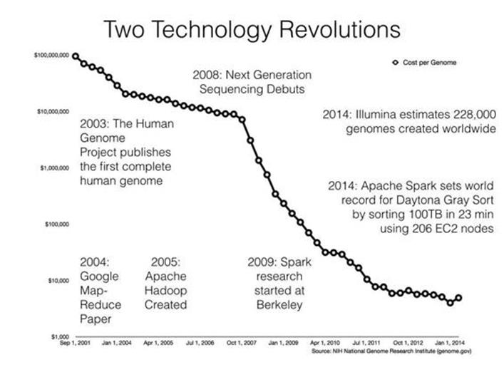
Figure 23-1. Timeline of big data technology and cost of sequencing a genome

The plummeting cost of sequencing points to superlinear growth of genomics data over the coming years. This DNA data deluge has left biological data scientists struggling to process data in a timely and scalable way using current genomics software. The AMPLab is a research lab in the Computer Science Division at UC Berkeley focused on creating novel big data systems and applications. For example, Apache Spark (see Chapter 19) is one system that grew out of the AMPLab. Spark recently broke the world record for the Daytona Gray Sort, sorting 100 TB in just 23 minutes. The team at Databricks that broke the record also demonstrated they could sort 1 PB in less than 4 hours!

Consider this amazing possibility: we have technology today that could analyze every genome collected in 2014 on the order of days using a few hundred machines.

While the AMPLab identified genomics as the ideal big data application for technical reasons, there are also more important compassionate reasons: the timely processing of biological data saves lives. This short use case will focus on systems we use and have developed, with our partners and the open source community, to quickly analyze large biological datasets.

The Structure of DNA

The discovery in 1953 by Francis Crick and James D. Watson, using experimental data collected by Rosalind Franklin and Maurice Wilkins, that DNA has a double helix structure was one of the greatest scientific discoveries of the 20th century. Their Nature article entitled “Molecular Structure of Nucleic Acids: A Structure for Deoxyribose Nucleic Acid” contains one of the most profound and understated sentences in science:

It has not escaped our notice that the specific pairing we have postulated immediately suggests a possible copying mechanism for the genetic material.

This “specific pairing” referred to the observation that the bases adenine (A) and thymine (T) always pair together and guanine (G) and cytosine (C) always pair together; see Figure 23-2. This deterministic pairing enables a “copying mechanism”: the DNA double helix unwinds and complementary base pairs snap into place, creating two exact copies of the original DNA strand.

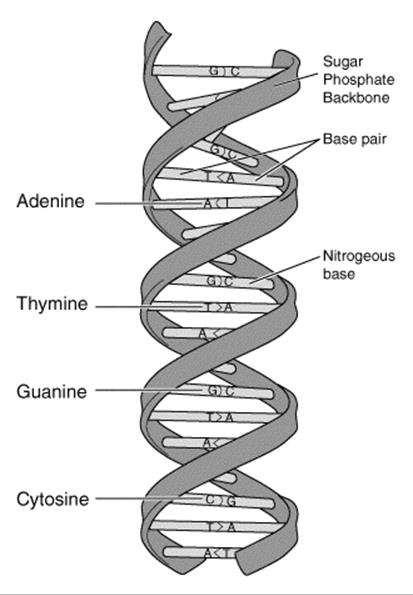
Figure 23-2. DNA double helix structure

The Genetic Code: Turning DNA Letters into Proteins

Without proteins, there is no life. DNA serves as a recipe for creating proteins. A protein is a chain of amino acids that folds into a specific 3D shape^[153^] to serve a particular structure or function. As there are a total of 20 amino acids^[154^] and only four letters in the DNA alphabet (A, C, T, G), nature groups these letters in words, called codons. Each codon is three bases long (since two bases would only support 4²=16 amino acids).

In 1968, Har Gobind Khorana, Robert W. Holley, and Marshall Nirenberg received the Nobel Prize in Physiology or Medicine for successfully mapping amino acids associated with each of the 64 codons. Each codon encodes a single amino acid, or designates the start and stop positions (see Table 23-1). Since there are 64 possible codons and only 20 amino acids, multiple codons correspond to some of the amino acids.

Table 23-1. Codon table

Because every organism on Earth evolved from the same common ancestor, every organism on Earth uses the same genetic code, with few variations. Whether the organism is a tree, worm, fungus, or cheetah, the codon UGG encodes tryptophan. Mother Nature has been the ultimate practitioner of code reuse over the last few billion years.

DNA is not directly used to synthesize amino acids. Instead, a process called transcription copies the DNA sequence that codes for a protein into messenger RNA (mRNA). These mRNA carry information from the nuclei of your cells to the surrounding cytoplasm to create proteins in a process called translation.

You probably noticed that this lookup table doesn’t have the DNA letter T (for thymine) and has a new letter U (for uracil). During transcription, U is substituted for T:

$ echo "ATGGTGACTCCTACATGA" | sed 's/T/U/g' | fold -w 3

AUG

GUG

ACU

CCU

ACA

UGA

Looking up these codons in the codon table, we can determine that this particular DNA strand will translate into a protein with the following amino acids in a chain: methionine, valine, threonine, proline, and threonine. This is a contrived example, but it logically demonstrates how DNA instructs the creation of proteins that make you uniquely you. It’s a marvel that science has allowed us to understand the language of DNA, including the start and stop punctuations.

Thinking of DNA as Source Code

At the cellular level, your body is a completely distributed system. Nothing is centralized. It’s like a cluster of 37.2 trillion^[155^] cells executing the same code: your DNA.

If you think of your DNA as source code, here are some things to consider:

§ The source is comprised of only four characters: A, C, T, and G.

§ The source has two contributors, your mother and father, who contributed 3.2 billion letters each. In fact, the reference genome provided by the Genome Reference Consortium (GRC) is nothing more than an ASCII file with 3.2 billion characters inside.^[156^]

§ The source is broken up into 25 separate files called chromosomes that each hold varying fractions of the source. The files are numbered, and tend to get smaller in size, with chromosome 1 holding ~250 million characters and chromosome 22 holding only ~50 million. There are also the X, Y, and mitochondrial chromosomes. The term chromosome basically means “colored thing,” from a time when biologists could stain them but didn’t know what they were.

§ The source is executed on your biological machinery three letters (i.e., a codon) at a time, using the genetic code explained previously — not unlike a Turing machine that reads chemical letters instead of paper ribbon.

§ The source has about 20,000 functions, called genes, which each create a protein when executed. The location of each gene in the source is called the locus. You can think of a gene as a specific range of contiguous base positions on a chromosome. For example, the BRCA1 gene implicated in breast cancer can be found on chromosome 17 from positions 41,196,312 to 41,277,500. A gene is like a “pointer” or “address,” whereas alleles (described momentarily) are the actual content. Everyone has the BRCA1 gene, but not everyone has alleles that put them at risk.

§ A haplotype is similar to an object in object-oriented programming languages that holds specific functions (genes) that are typically inherited together.

§ The source has two definitions for each gene, called alleles — one from your mother and one from your father — which are found at the same position of paired chromosomes (while the cells in your body are diploid — that is, they have two alleles per gene — there are organisms that are triploid, tetraploid, etc.). Both alleles are executed and the resultant proteins interact to create a specific phenotype. For example, proteins that make or degrade eye color pigment lead to a particular phenotype, or an observable characteristic (e.g., blue eyes). If the alleles you inherit from your parents are identical, you’re homozygous for that allele; otherwise, you’re heterozygous.

§ A single-nucleic polymorphism (SNP), pronounced “snip,” is a single-character change in the source code (e.g., from ACTGACTG to ACTTACTG).

§ An indel is short for insert-delete and represents an insertion or deletion from the reference genome. For example, if the reference has CCTGACTG and your sample has four characters inserted — say, CCTGCCTAACTG — then it is an indel.

§ Only 0.5% of the source gets translated into the proteins that sustain your life. That portion of the source is called your exome. A human exome requires a few gigabytes to store in compressed binary files.

§ The other 99.5% of the source is commented out and serves as word padding (introns); it is used to regulate when genes are turned on, repeat, and so on.^[157^] A whole genome requires a few hundred gigabytes to store in compressed binary files.

§ Every cell of your body has the same source,^[158^] but it can be selectively commented out by epigenetic factors like DNA methylation and histone modification, not unlike an #ifdef statement for each cell type (e.g., #ifdef RETINA or #ifdef LIVER). These factors are responsible for making cells in your retina operate differently than cells in your liver.

§ The process of variant calling is similar to running diff between two different DNA sources.

These analogies aren’t meant to be taken too literally, but hopefully they helped familiarize you with some genomics terminology.

The Human Genome Project and Reference Genomes

In 1953, Watson and Crick discovered the structure of DNA, and in 1965 Nirenberg, with help from his NIH colleagues, cracked the genetic code, which expressed the rules for translating DNA or mRNA into proteins. Scientists knew that there were millions of human proteins but didn’t have a complete survey of the human genome, which made it impossible to fully understand the genes responsible for protein synthesis. For example, if each protein was created by a single gene, that would imply millions of protein-coding genes in the human genome.

In 1990, the Human Genome Project set out to determine all the chemical base pairs that make up human DNA. This collaborative, international research program published the first human genome in April of 2003,^[159^] at an estimated cost of $3.8 billion. The Human Genome Project generated an estimated $796 billion in economic impact, equating to a return on investment (ROI) of 141:1.^[160^] The Human Genome Project found about 20,500 genes — significantly fewer than the millions you would expect with a simple 1:1 model of gene to protein, since proteins can be assembled from a combination of genes, post-translational processes during folding, and other mechanisms.

While this first human genome took over a decade to build, once created, it made “bootstrapping” the subsequent sequencing of other genomes much easier. For the first genome, scientists were operating in the dark. They had no reference to search as a roadmap for constructing the full genome. There is no technology to date that can read a whole genome from start to finish; instead, there are many techniques that vary in the speed, accuracy, and length of DNA fragments they can read. Scientists in the Human Genome Project had to sequence the genome in pieces, with different pieces being more easily sequenced by different technologies. Once you have a complete human genome, subsequent human genomes become much easier to construct; you can use the first genome as a reference for the second. The fragments from the second genome can be pattern matched to the first, similar to having the picture on a jigsaw puzzle’s box to help inform the placement of the puzzle pieces. It helps that most coding sequences are highly conserved, and variants only occur at 1 in 1,000 loci.

Shortly after the Human Genome Project was completed, the Genome Reference Consortium (GRC), an international collection of academic and research institutes, was formed to improve the representation of reference genomes. The GRC publishes a new human reference that serves as something like a common coordinate system or map to help analyze new genomes. The latest human reference genome, released in February 2014, was named GRCh38; it replaced GRCh37, which was released five years prior.

Sequencing and Aligning DNA

Second-generation sequencing is rapidly evolving, with numerous hardware vendors and new sequencing methods being developed about every six months; however, a common feature of all these technologies is the use of massively parallel methods, where thousands or even millions of reactions occur simultaneously. The double-stranded DNA is split down the middle, the single strands are copied many times, and the copies are randomly shredded into small fragments of different lengths called reads, which are placed into the sequencer. The sequencer reads the “letters” in each of these reads, in parallel for high throughput, and outputs a raw ASCII file containing each read (e.g., AGTTTCGGGATC...), as well as a quality estimate for each letter read, to be used for downstream analysis.

A piece of software called an aligner takes each read and works to find its position in the reference genome (see Figure 23-3).^[161^] A complete human genome is about 3 billion base (A, C, T, G) pairs long.^[162^] The reference genome (e.g., GRCh38) acts like the picture on a puzzle box, presenting the overall contours and colors of the human genome. Each short read is like a puzzle piece that needs to be fit into position as closely as possible. A common metric is “edit distance,” which quantifies the number of operations necessary to transform one string to another. Identical strings have an edit distance of zero, and an indel of one letter has an edit distance of one. Since humans are 99.9% identical to one another, most of the reads will fit to the reference quite well and have a low edit distance. The challenge with building a good aligner is handling idiosyncratic reads.

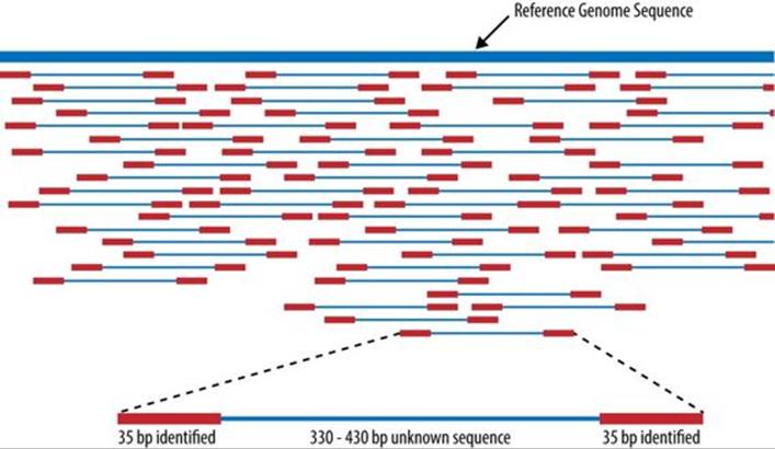
Figure 23-3. Aligning reads to a reference genome, from Wikipedia

ADAM, A Scalable Genome Analysis Platform

Aligning the reads to a reference genome is only the first of a series of steps necessary to generate reports that are useful in a clinical or research setting. The early stages of this processing pipeline look similar to any other extract-transform-load (ETL) pipelines that need data deduplication and normalization before analysis.

The sequencing process duplicates genomic DNA, so it’s possible that the same DNA reads are generated multiple times; these duplicates need to be marked. The sequencer also provides a quality estimate for each DNA “letter” that it reads, which has sequencer-specific biases that need to be adjusted. Aligners often misplace reads that have indels (inserted or deleted sequences) that need to be repositioned on the reference genome. Currently, this preprocessing is done using single-purpose tools launched by shell scripts on a single machine. These tools take multiple days to finish the processing of whole genomes. The process is disk bound, with each stage writing a new file to be read into subsequent stages, and is an ideal use case for applying general-purpose big data technology. ADAM is able to handle the same preprocessing in under two hours.

ADAM is a genome analysis platform that focuses on rapidly processing petabytes of high-coverage, whole genome data. ADAM relies on Apache Avro, Parquet, and Spark. These systems provide many benefits when used together, since they:

§ Allow developers to focus on algorithms without needing to worry about distributed system failures

§ Enable jobs to be run locally on a single machine, on an in-house cluster, or in the cloud without changing code

§ Compress legacy genomic formats and provide predicate pushdown and projection for performance

§ Provide an agile way of customizing and evolving data formats

§ Are designed to easily scale out using only commodity hardware

§ Are shared with a standard Apache 2.0 license^[163^]

Literate programming with the Avro interface description language (IDL)

The Sequence Alignment/Map (SAM) specification defines the mandatory fields listed in Table 23-2.

Table 23-2. Mandatory fields in the SAM format

Any developers who want to implement this specification need to translate this English spec into their computer language of choice. In ADAM, we have chosen instead to use literate programming with a spec defined in Avro IDL. For example, the mandatory fields for SAM can be easily expressed in a simple Avro record:

record AlignmentRecord {

string qname;

int flag;

string rname;

int pos;

int mapq;

string cigar;

string rnext;

int pnext;

int tlen;

string seq;

string qual;

}

Avro is able to autogenerate native Java (or C++, Python, etc.) classes for reading and writing data and provides standard interfaces (e.g., Hadoop’s InputFormat) to make integration with numerous systems easy. Avro is also designed to make schema evolution easier. In fact, theADAM schemas we use today have evolved to be more sophisticated, expressive, and customized to express a variety of genomic models such as structural variants, genotypes, variant calling annotations, variant effects, and more.

UC Berkeley is a member of the Global Alliance for Genomics & Health, a non-governmental, public-private partnership consisting of more than 220 organizations across 30 nations, with the goal of maximizing the potential of genomics medicine through effective and responsible data sharing. The Global Alliance has embraced this literate programming approach and publishes its schemas in Avro IDL as well. Using Avro has allowed researchers around the world to talk about data at the logical level, without concern for computer languages or on-disk formats.

Column-oriented access with Parquet

The SAM and BAM^[164^] file formats are row-oriented: the data for each record is stored together as a single line of text or a binary record. (See Other File Formats and Column-Oriented Formats for further discussion of row- versus column-oriented formats.) A single paired-end read in a SAM file might look like this:

read1 99 chrom1 7 30 8M2I4M1D3M = 37 39 TTAGATAAAGGATACTG *

read1 147 chrom1 37 30 9M = 7 -39 CAGCGGCAT * NM:i:1

A typical SAM/BAM file contains many millions of rows, one for each DNA read that came off the sequencer. The preceding text fragment translates loosely into the view shown in Table 23-3.

Table 23-3. Logical view of SAM fragment

In this example, the read, identified as read1, was mapped to the reference genome at chromosome1, positions 7 and 37. This is called a “paired-end” read as it represents a single strand of DNA that was read from each end by the sequencer. By analogy, it’s like reading an array of length 150 from 0..50 and 150..100.

The MapQ score represents the probability that the sequence is mapped to the reference correctly. MapQ scores of 20, 30, and 40 have a probability of being correct of 99%, 99.9%, and 99.99%, respectively. To calculate the probability of error from a MapQ score, use the expression 10^(-MapQ/10) (e.g., 10^(-30/10) is a probability of 0.001).

The CIGAR explains how the individual nucleotides in the DNA sequence map to the reference.^[165^] The Sequence is, of course, the DNA sequence that was mapped to the reference.

There is a stark mismatch between the SAM/BAM row-oriented on-disk format and the column-oriented access patterns common to genome analysis. Consider the following:

§ A range query to find data for a particular gene linked to breast cancer, named BRCA1: “Find all reads that cover chromosome 17 from position 41,196,312 to 41,277,500”

§ A simple filter to find poorly mapped reads: “Find all reads with a MapQ less than 10”

§ A search of all reads with insertions or deletions, called indels: “Find all reads that contain I or D in the CIGAR string”

§ Count the number of unique k-mers: “Read every Sequence and generate all possible substrings of length k in the string”

Parquet’s predicate pushdown feature allows us to rapidly filter reads for analysis (e.g., finding a gene, ignoring poorly mapped reads). Projection allows for precise materialization of only the columns of interest (e.g., reading only the sequences for k-mer counting).

Additionally, a number of the fields have low cardinality, making them ideal for data compression techniques like run-length encoding (RLE). For example, given that humans have only 23 pairs of chromosomes, the Reference field will have only a few dozen unique values (e.g.,chromosome1, chromosome17, etc.). We have found that storing BAM records inside Parquet files results in ~20% compression. Using the PrintFooter command in Parquet, we have found that quality scores can be run-length encoded and bit-packed to compress ~48%, but they still take up ~70% of the total space. We’re looking forward to Parquet 2.0, so we can use delta encoding on the quality scores to compress the file size even more.

A simple example: k-mer counting using Spark and ADAM

Let’s do “word count” for genomics: counting k-mers. The term k-mers refers to all the possible subsequences of length k for a read. For example, if you have a read with the sequence AGATCTGAAG, the 3-mers for that sequence would be ['AGA', 'GAT', 'ATC', 'TCT', 'CTG', 'TGA', 'GAA', 'AAG']. While this is a trivial example, k-mers are useful when building structures like De Bruijn graphs for sequence assembly. In this example, we are going to generate all the possible 21-mers from our reads, count them, and then write the totals to a text file.

This example assumes that you’ve already created a SparkContext named sc. First, we create a Spark RDD of AlignmentRecords using a pushdown predicate to remove low-quality reads and a projection to only materialize the sequence field in each read:

// Load reads from 'inputPath' into an RDD for analysis

val adamRecords: RDD[AlignmentRecord] = sc.adamLoad(args.inputPath,

// Filter out all low-quality reads that failed vendor quality checks

predicate = Some(classOf[HighQualityReadsPredicate]),

// Only materialize the 'sequence' from each record

projection = Some(Projection(AlignmentRecordField.sequence)))

Since Parquet is a column-oriented storage format, it can rapidly materialize only the sequence column and quickly skip over the unwanted fields. Next, we walk over each sequence using a sliding window of length k=21, emit a count of 1L, and then reduceByKey using the k-mer subsequence as the key to get the total counts for the input file:

// The length of k-mers we want to count

val kmerLength = 21

// Process the reads into an RDD of tuples with k-mers and counts

val kmers: RDD[(String, Long)] = adamRecords.flatMap(read => {

read.getSequence

.toString

.sliding(kmerLength)

.map(k => (k, 1L))

}).reduceByKey { case (a, b) => a + b}

// Print the k-mers as a text file to the 'outputPath'

kmers.map { case (kmer, count) => s"$count,$kmer"}

.saveAsTextFile(args.outputPath)

When run on sample NA21144, chromosome 11 in the 1000 Genomes project,^[166^] this job outputs the following:

AAAAAAAAAAAAAAAAAAAAAA, 124069

TTTTTTTTTTTTTTTTTTTTTT, 120590

ACACACACACACACACACACAC, 41528

GTGTGTGTGTGTGTGTGTGTGT, 40905

CACACACACACACACACACACA, 40795

TGTGTGTGTGTGTGTGTGTGTG, 40329

TAATCCCAGCACTTTGGGAGGC, 32122

TGTAATCCCAGCACTTTGGGAG, 31206

CTGTAATCCCAGCACTTTGGGA, 30809

GCCTCCCAAAGTGCTGGGATTA, 30716

...

ADAM can do much more than just count k-mers. Aside from the preprocessing stages already mentioned — duplicate marking, base quality score recalibration, and indel realignment — it also:

§ Calculates coverage read depth at each variant in a Variant Call Format (VCF) file

§ Counts the k-mers/q-mers from a read dataset

§ Loads gene annotations from a Gene Transfer Format (GTF) file and outputs the corresponding gene models

§ Prints statistics on all the reads in a read dataset (e.g., % mapped to reference, number of duplicates, reads mapped cross-chromosome, etc.)

§ Launches legacy variant callers, pipes reads into stdin, and saves output from stdout

§ Comes with a basic genome browser to view reads in a web browser

However, the most important thing ADAM provides is an open, scalable platform. All artifacts are published to Maven Central (search for group ID org.bdgenomics) to make it easy for developers to benefit from the foundation ADAM provides. ADAM data is stored in Avro and Parquet, so you can also use systems like SparkSQL, Impala, Apache Pig, Apache Hive, or others to analyze the data. ADAM also supports job written in Scala, Java, and Python, with more language support on the way.

At Scala.IO in Paris in 2014, Andy Petrella and Xavier Tordoir used Spark’s MLlib k-means with ADAM for population stratification across the 1000 Genomes dataset (population stratification is the process of assigning an individual genome to an ancestral group). They found that ADAM/Spark improved performance by a factor of 150.

From Personalized Ads to Personalized Medicine

While ADAM is designed to rapidly and scalably analyze aligned reads, it does not align the reads itself; instead, ADAM relies on standard short-reads aligners. The Scalable Nucleotide Alignment Program (SNAP) is a collaborative effort including participants from Microsoft Research, UC San Francisco, and the AMPLab as well as open source developers, shared with an Apache 2.0 license. The SNAP aligner is as accurate as the current best-of-class aligners, like BWA-mem, Bowtie2, and Novalign, but runs between 3 and 20 times faster. This speed advantage is important when doctors are racing to identify a pathogen.

In 2013, a boy went to the University of Wisconsin Hospital and Clinics’ Emergency Department three times in four months with symptoms of encephalitis: fevers and headaches. He was eventually hospitalized without a successful diagnosis after numerous blood tests, brain scans, and biopsies. Five weeks later, he began having seizures that required he be placed into a medically induced coma. In desperation, doctors sampled his spinal fluid and sent it to an experimental program led by Charles Chiu at UC San Francisco, where it was sequenced for analysis. The speed and accuracy of SNAP allowed UCSF to quickly filter out all human DNA and, from the remaining 0.02% of the reads, identify a rare infectious bacterium, Leptospira santarosai. They reported the discovery to the Wisconsin doctors just two days after they sent the sample. The boy was treated with antibiotics for 10 days, awoke from his coma, and was discharged from the hospital two weeks later.^[167^]

If you’re interested in learning more about the system the Chiu lab used — called Sequence-based Ultra-Rapid Pathogen Identification (SURPI) — they have generously shared their software with a permissive BSD license and provide an Amazon EC2 Machine Image (AMI) with SURPI preinstalled. SURPI collects 348,922 unique bacterial sequences and 1,193,607 unique virus sequences from numerous sources and saves them in 29 SNAP-indexed databases, each approximately 27 GB in size, for fast search.

Today, more data is analyzed for personalized advertising than personalized medicine, but that will not be the case in the future. With personalized medicine, people receive customized healthcare that takes into consideration their unique DNA profiles. As the price of sequencing drops and more people have their genomes sequenced, the increase in statistical power will allow researchers to understand the genetic mechanisms underlying diseases and fold these discoveries into the personalized medical model, to improve treatment for subsequent patients. While only 25 PB of genomic data were generated worldwide this year, next year that number will likely be 100 PB.

Join In

While we’re off to a great start, the ADAM project is still an experimental platform and needs further development. If you’re interested in learning more about programming on ADAM or want to contribute code, take a look at Advanced Analytics with Spark: Patterns for Learning from Data at Scale by Sandy Ryza et al. (O’Reilly, 2014), which includes a chapter on analyzing genomics data with ADAM and Spark. You can find us at http://bdgenomics.org, on IRC at #adamdev, or on Twitter at @bigdatagenomics.

^[152^] See Antonio Regalado, “EmTech: Illumina Says 228,000 Human Genomes Will Be Sequenced This Year,” September 24, 2014.

^[153^] This process is called protein folding. The Folding@home allows volunteers to donate CPU cycles to help researchers determine the mechanisms of protein folding.

^[154^] There are also a few nonstandard amino acids not shown in the table that are encoded differently.

^[155^] See Eva Bianconi et al., “An estimation of the number of cells in the human body,” Annals of Human Biology, November/December 2013.

^[156^] You might expect this to be 6.4 billion letters, but the reference genome is, for better or worse, a haploid representation of the average of dozens of individuals.

^[157^] Only about 28% of your DNA is transcribed into nascent RNA, and after RNA splicing, only about 1.5% of the RNA is left to code for proteins. Evolutionary selection occurs at the DNA level, with most of your DNA providing support to the other 0.5% or being deselected altogether (as more fitting DNA evolves). There are some cancers that appear to be caused by dormant regions of DNA being resurrected, so to speak.

^[158^] There is actually, on average, about 1 error for each billion DNA “letters” copied. So, each cell isn’t exactly the same.

^[159^] Intentionally 50 years after Watson and Crick’s discovery of the 3D structure of DNA.

^[160^] Jonathan Max Gitlin, “Calculating the economic impact of the Human Genome Project,” June 2013.

^[161^] There is also a second approach, de novo assembly, where reads are put into a graph data structure to create long sequences without mapping to a reference genome.

^[162^] Each base is about 3.4 angstroms, so the DNA from a single human cell stretches over 2 meters end to end!

^[163^] Unfortunately, some of the more popular software in genomics has an ill-defined or custom, restrictive license. Clean open source licensing and source code are necessary for science to make it easier to reproduce and understand results.

^[164^] BAM is the compressed binary version of the SAM format.

^[165^] The first record’s Compact Idiosyncratic Gap Alignment Report (CIGAR) string is translated as “8 matches (8M), 2 inserts (2I), 4 matches (4M), 1 delete (1D), 3 matches (3M).”

^[166^] Arguably the most popular publicly available dataset, found at http://www.1000genomes.org.

^[167^] Michael Wilson et al., “Actionable Diagnosis of Neuroleptospirosis by Next-Generation Sequencing,” New England Journal of Medicine, June 2014.