Professional Microsoft SQL Server 2014 Integration Services (Wrox Programmer to Programmer), 1st Edition (2014)

Chapter 15. Reliability and Scalability

WHAT’S IN THIS CHAPTER?

· Restarting packages

· Using package transactions for data consistency

· Using error outputs for reliability and scalability

· Scaling out efficiently and reliably

WROX.COM CODE DOWNLOADS FOR THIS CHAPTER

You can find the wrox.com code downloads for this chapter at http://www.wrox.com/go/prossis2014 on the Download Code tab.

Reliability and scalability are goals for all your systems, and although it may seem strange to combine them in one chapter, they are often directly linked, as you will see. Errors and the unexpected conditions that precipitate them are the most obvious threats to a reliable process. Several features of SQL Server 2014 Integration Services enable you to handle these situations with grace and integrity, keeping the data moving and the systems running.

Error outputs and checkpoints are the two features you will focus on in this chapter, and you will see how they can be used in the context of reliability. Implementation of these methods can also have a direct effect on package performance, and therefore scalability, and you will learn how to take into account these considerations for your package and process design. The capability to provide checkpoints does not natively extend inside the Data Flow Task, but there are methods you can apply to achieve this. The methods can then be transferred almost directly into the context of scalability, enabling you to partition packages and improve both reliability and scalability at the same time. All of these methods can be combined, and while there is no one-size-fits-all solution, this chapter describes all your options so you have the necessary information to make informed choices for your own SSIS implementations.

RESTARTING PACKAGES

Everyone has been there — one of your Data Transformation Services (DTS) packages failed overnight, and you now have to completely rerun the package. This is particularly painful if some of the processes inside the package are expensive in terms of resources or time. In DTS, it wasn’t possible to restart a package from where it left off, and picking apart a package to run just those tasks that failed was tedious and error prone. A variety of exotic solutions have been used, such as a post-execution process that goes into the package and recreates the package from the failed step forward. Although this worked, it required someone with a detailed knowledge of the DTS object model, which most production DBAs did not have. If your process takes data from a production SQL Server that has a very small window of ETL opportunity, you can be sure that most DBAs are not going to be pleased when you tell them you need to run the extract again, and that it may impact the users.

For this reason, “package restartability” or checkpoints in SQL Server Integration Services was a huge relief. In this chapter, you are going to learn everything you need to know to enable restartability in your SSIS packages.

Checkpoints are the foundation for restarting packages in SSIS, and they work by writing state information to a file after each task completes. This file can then be used to determine which tasks have run and which have failed. More detail about these files is provided in the “Inside the Checkpoint File” section. To ensure that the checkpoint file is created correctly, you must set three package properties and one task property, which can be found on the property pages of the package and task. The package properties are as follows:

· CheckpointFilename: This is the filename of the checkpoint file, which must be provided. There are no specific conventions or requirements for the filename.

· CheckpointUsage: There are three values, which describe how a checkpoint file is used during package execution:

· Never: The package will not use a checkpoint file and therefore will never restart.

· If Exists: If a checkpoint file exists in the place you specified for the CheckpointFilename property, then it will be used, and the package will restart according to the checkpoints written.

· Always: The package will always use a checkpoint file to restart; if one does not exist, the package will fail.

· SaveCheckpoints: This is a simple Boolean to indicate whether checkpoints are to be written. Obviously, this must be set to true for this scenario.

The one property you have to set on the task is FailPackageOnFailure. This must be set for each task or container that you want to be the point for a checkpoint and restart. If you do not set this property to true and the task fails, no file will be written, and the next time you invoke the package, it will start from the beginning again. You’ll see an example of this happening later.

NOTE As you know, SSIS packages are broken down into the Control Flow and Data Flow Tasks. Checkpoints occur only at the Control Flow; it is not possible to checkpoint transformations or restart inside a Data Flow Task. The Data Flow Task can be a checkpoint, but it is treated like any other task. This ensures Data Flow Tasks write all or none of their data, like a SQL transaction with commits and rollbacks. Implementing your own checkpoint and restart feature for data is described later in the chapter.

Keep in mind that if nothing fails in your package, no file will be generated. You’ll have a look later at the generated file itself and try to make some sense out of it, but for now you only need to know that the file contains all the information needed by the package when it is restarted, enabling it to behave like nothing untoward had interrupted it. That’s enough information to be able to start using checkpoints in your packages, so now you can proceed with some examples.

Simple Control Flow

The first example package you will create contains a simple Control Flow with a series of tasks meant to highlight the power of checkpoints. Create a package named Checkpoint.dtsx that contains three Execute SQL Tasks, as shown in Figure 15-1.

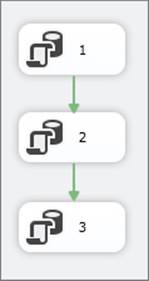
FIGURE 15-1

In the new package, add a connection manager to the AdventureWorksDW database. Then, add a simple select statement, such as “select 1” to the first and third tasks. The second of these tasks, aptly named “2,” is set to fail with a divide-by-zero error, as shown in the Task Editor in Figure 15-2.

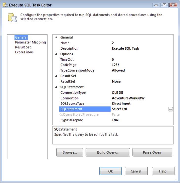
FIGURE 15-2

Assume that the task labeled “1” is expensive, and you want to ensure that you don’t need to execute it twice if it finishes and something else in the package fails. You now need to set up the package to use checkpoints and the task itself. First, set the properties of the package described earlier, as shown in Figure 15-3.

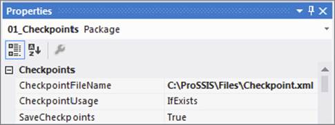
FIGURE 15-3

Next, set the properties of the task labeled “2” to use checkpoints (see Figure 15-4). Change the FailPackageOnFailure property to True.

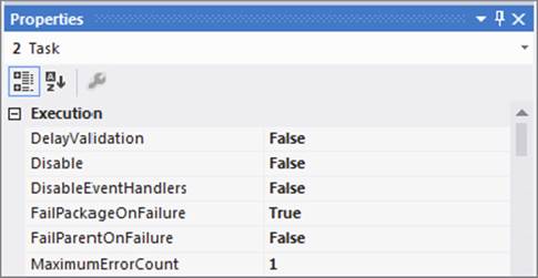
FIGURE 15-4

Now you can execute the package. The expected outcome is shown in Figure 15-5 — the first task completes successfully with a check mark in a green circle, but the second task fails with an X in a red circle. The third task did not execute. Because the screenshots for this book are in black and white, you won’t be able to see the colors here, but you can see that the tasks contain different symbols in the top-right corner.

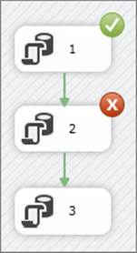
FIGURE 15-5

If you had created this package in DTS, you would have had to write some logic to cope with the failure in order to not have to execute task 1 again. Because you are working in SSIS and have set the package up properly, you can rely on checkpoints. When the package failed, the error output window said something like this:

SSIS package "C:\ProSSIS\Code\Ch15\01_Checkpoints.dtsx" starting.

Information: 0x40016045 at 01_Checkpoints: The package will be saving checkpoints to file "C:\ProSSIS\Files\Checkpoint.xml" during execution. The package is configured to save checkpoints.

Information: 0x40016049 at 01_Checkpoints: Checkpoint file "C:\ProSSIS\Files\Checkpoint.xml" update starting.

Information: 0x40016047 at 1: Checkpoint file "C:\ProSSIS\Files\Checkpoint.xml" was updated to record completion of this container.

Error: 0xC002F210 at 2, Execute SQL Task: Executing the query "Select 1/0" failed with the following error: "Divide by zero error encountered.". Possible failure reasons: Problems with the query, "ResultSet" property not set correctly, parameters not set correctly, or connection not established correctly.

Task failed: 2

SSIS package "C:\ProSSIS\Code\Ch15\01_Checkpoints.dtsx" finished: Failure.

As you can see, the output window says that a checkpoint file was written. If you look at the file system, you can see that this is true, as shown in Figure 15-6. You’ll look inside the file later when you have a few more things of interest in there, but for the moment just understand that the package now knows what happened and where.

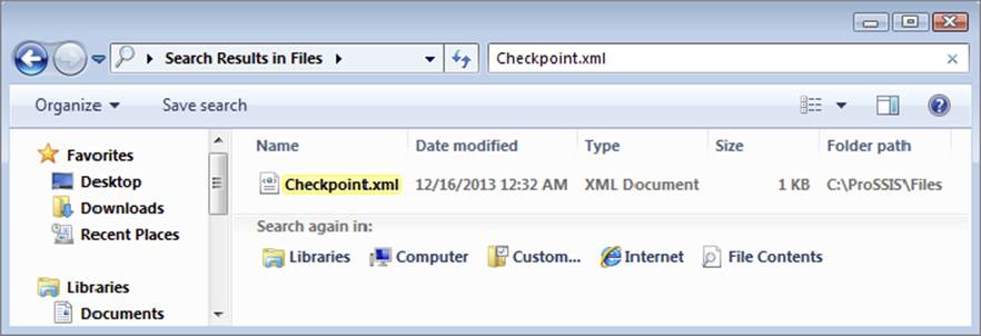
FIGURE 15-6

Now you need to fix the problem by removing the divide-by-zero issue in the second task (change the SQL Statement to Select 1 instead of Select 1/0) and run the package again. Figure 15-7 shows what happens after you do that.

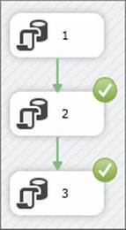
FIGURE 15-7

Task 2 was executed again and then task 3. Task 1 was oblivious to the package running again.

Recall from earlier that the task you want to be the site for a checkpoint must have the FailPackageOnFailure property set to true. Otherwise, no file will be written; and when the package executes again it will start from the beginning. Here is how that works. Set task 2 to not use checkpoints by setting this property to false, as shown in Figure 15-8.

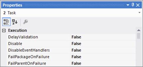
FIGURE 15-8

Change the SQL Statement in task 2 back to Select 1/0 and then execute the package again. No checkpoint file is written, as expected. This means that after you fix the error in the task again and rerun the package one more time, the results look like Figure 15-9; all tasks have a green check mark in the top right corner, which may or may not be what you want.

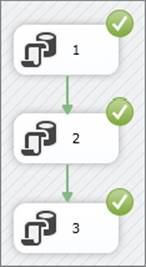
FIGURE 15-9

This example is a very simple one that involves only three tasks joined by a workflow, but hopefully it has given you an idea about restartability in SSIS packages; the examples that follow are more complicated.

Containers within Containers and Checkpoints

Containers and transactions have an effect on checkpoints. You will see these effects in this example, and change some properties and settings while you’re at it. First, you will create a new package named ContainerCheckpoints.dtsx using Sequence Containers and checkpoints. In this package you have two Sequence Containers, which themselves contain Execute SQL Tasks, as shown in Figure 15-10.

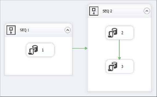
FIGURE 15-10

Make sure the package has all the settings necessary to use checkpoints, as in the previous example. On the initial run-through of this package, the only container that you want to be the site for a checkpoint is task 3, so set the FailPackageOnFailure property of task 3 to true. Figure 15-11 shows what happens when you deliberately set this task to fail, perhaps with a divide-by-zero error (refer to the previous example to see how to do that).

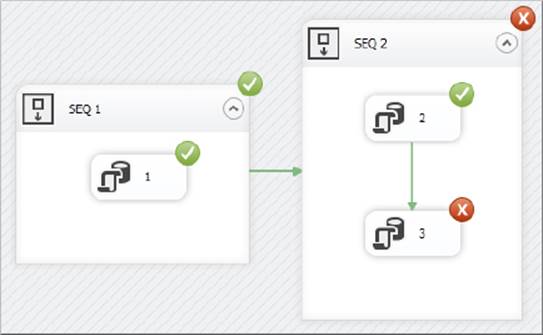
FIGURE 15-11

As expected, task 3 has failed, and the Sequence Container, SEQ 2, has also failed because of this. If you now fix the problem with task 3 and re-execute the package, you will see results matching those shown in Figure 15-12.

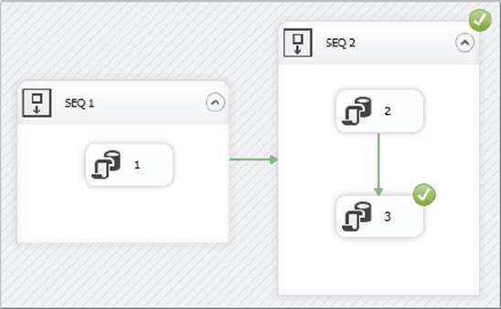
FIGURE 15-12

Therefore, there’s no real difference here from the earlier example except that the Sequence Container “SEQ 2” has a green check. Now you’ll change the setup of the package to see the behavior change dramatically. What you’re going to do is make the Sequence Container SEQ 2 transacted. That means you’re going to wrap SEQ 2 and its child containers in a transaction. Change the properties of the SEQ 2 container to look like Figure 15-13 so that the TransactionOption property is set to Required.

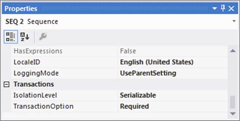
FIGURE 15-13

Setting the TransactionOption property of the SEQ 2 container to Required means that it will start its own transaction. Now open the properties window of the two child Execute SQL Tasks and set their TransactionOption properties to Supported, as shown in Figure 15-14, so that they will join a transaction if one exists.

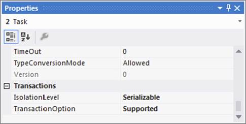
FIGURE 15-14

WARNING SSIS uses the Microsoft Distributed Coordinator to manage its transactions. Before setting the TransactionOption property to Required, be sure to start Microsoft Distributed Transaction Coordinator (MSDTC) service.

Now execute the package again. On the first run-through, the package fails as before at task 3. The difference occurs when you fix the problem with task 3 and re-execute the package. The result looks like Figure 15-15.

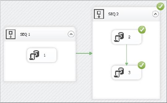
FIGURE 15-15

Because the container was transacted, the fact that task 3 failed is not recorded in the checkpoint file. Instead, the fact that the Sequence Container failed is recorded; hence, the Sequence Container is re-executed in its entirety when the package is rerun. Therefore, tasks 2 and 3 execute on the second run. Note that the transaction was on the Sequence Container and not the individual tasks. If you have a set of tasks that need to be run in a transaction, the Sequence Container will handle this for you.

Variations on a Theme

You may have noticed another property in the task property pages next to the FailPackageOnFailure property — the FailParentOnFailure property. In the previous example, the SEQ 2 container is the parent to the two Execute SQL Tasks 2 and 3. You’ll run through a few variations of the parent/child relationship here so that you can see the differences. In each example, you will force a failure on the first run-through; then you will correct the problem and run the package a second time.

Failing the Parent, Not the Package

What happens if instead of setting the FailPackageOnFailure property of task 3 to true, you set the FailParentOnFailure property to true? After a failed execution and then issue resolution, the whole package will be run again on re-execution of the package. Why? Because no checkpoint file has been written.

NOTE Remember that if you want a checkpoint file to be written, the task that fails must have the FailPackageOnFailure property set to true; otherwise, no file is written.

Failing the Parent and the Package

In this variation, you still have a transacted Sequence Container, and you still have task 3’s FailParentOnFailure property set to true. In addition, set the SEQ 2 Sequence Container’s FailPackageOnFailure property to true. Figure 15-16 shows what happens on the rerun of the package after a failure.

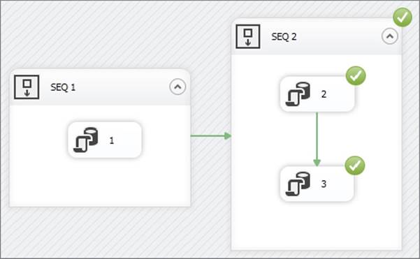
FIGURE 15-16

As you can see, the Sequence Container executes in its entirety, and the output window from the package confirms that you used a checkpoint file and started a transaction:

SSIS package "C:\ProSSIS\Code\Ch15\02_ContainerCheckpoints.dtsx" starting.

Information: 0x40016046 at 02_ContainerCheckpoints: The package restarted from checkpoint file "C:\ProSSIS\Files\ContainerCheckpoint.xml". The package was configured to restart from checkpoint.

Information: 0x40016045 at 02_ContainerCheckpoints: The package will be saving checkpoints to file "C:\ProSSIS\Files\ContainerCheckpoint.xml" during execution. The package is configured to save checkpoints.

Information: 0x4001100A at SEQ 2: Starting distributed transaction for this container.

Information: 0x4001100B at SEQ 2: Committing distributed transaction started by this container.

SSIS package "C:\ProSSIS\Code\Ch15\02_ContainerCheckpoints.dtsx" finished: Success.

Failing the Task with No Transaction

The next variation will show what happens if you set some of the checkpoint properties without having a transaction in place. Start by removing the transactions from your package by setting the SEQ 2’s TransactionOption property to Supported. Force an error in task 3, and run the package again to see it fail at task 3. Then, fix the problem, and re-execute the package. Remember that task 3 has its FailParentOnFailure property set to true, and the SEQ 2 Sequence Container has its FailPackageOnFailure set to true. The outcome, shown in Figure 15-17, is not exactly what you likely expected. As you can imagine, this is not very useful. The Sequence Container shows success, yet none of the tasks in the container executed. It’s important to ensure that you have the properties of the tasks and the containers set properly in order to ensure that the desired tasks execute after the checkpoint is created.

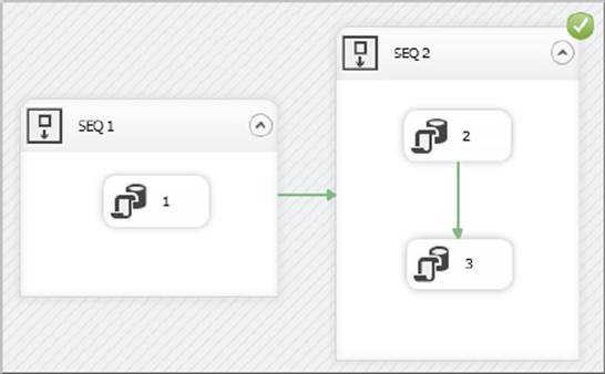
FIGURE 15-17

Failing the Package, Not the Sequence

You might assume that if tasks 2 and 3 have the Sequence Container as a parent, then the package itself must be the parent of the Sequence Container. If this is the case, wouldn’t setting FailParentOnFailure on the Sequence Container be the same as setting FailPackageOnFailure on the same container? The quick answer is no. If you try this, you will see that no checkpoint file is written, and by now you know what that means. The message here is that if you want a checkpoint file to be written, then make sure that the restart point has FailPackageOnFailure set to true.

Inside the Checkpoint File

As promised earlier, it’s time to look inside the checkpoint file to see what it contains now that you have more things to put in there. In the CheckpointScripts.dtsx package shown in Figure 15-18, although you have only three tasks, you also have a variable value being changed. The purpose of this package is to show you what kind of information is stored in a checkpoint file. To add a variable, simply click the designer while in the Control Flow and choose Variables from the SSIS menu or right-click on the Control Flow background and select Variables. Create a Variable named intVar and make the variable type integer. Leave the default value of zero.

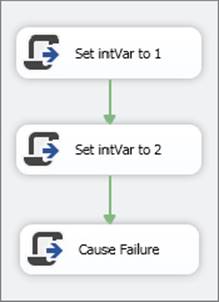
FIGURE 15-18

The Script Tasks will change the value of the intVar variable to 1 and then to 2, and the last Script Task will try to set the variable to the letter “x”. This will cause the last Script Task to fail because of nonmatching data types. To alter the value of a variable in all Script Tasks, you add the variable name to the ReadWriteVariables section on the Script Task’s editor. You then need to add some script to change the value. The following is the Visual Basic script in the first Script Task:

Public Sub Main()

Dts.Variables("intVar").Value = 1

Dts.TaskResult = ScriptResults.Success

End Sub

NOTE Code samples for this chapter can be found as part of the code download for this book available at http://www.wrox.com/go/prossis2014.

Now run the package. It will fail, as shown in Figure 15-19. A Script Task Error Window may appear. If so, just click Close.

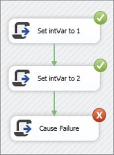
FIGURE 15-19

NOTE Instead of altering the Script Task code to make your task fail, you can simply set the ForceExecutionResult on the task to Failure. You can also do this on any Containers too.

Inside the generated checkpoint file, you should find something like this:

<DTS:Checkpoint xmlns:DTS="www.microsoft.com/SqlServer/Dts"

DTS:PackageID="{16EDDCF1-5141-44B6-8997-0A42EB82A767}">

<DTS:Variables DTS:ContID="{16EDDCF1-5141-44B6-8997-0A42EB82A767}">

<DTS:Variable DTS:Namespace="User" DTS:IncludeInDebugDump="6789"

DTS:ObjectName="intVar" DTS:DTSID="{4DA0C488-4CCA-4F33-B2FE-DAE1219A5A77}"

DTS:CreationName="">

<DTS:VariableValue DTS:DataType="3">2</DTS:VariableValue>

</DTS:Variable>

</DTS:Variables>

<DTS:Container DTS:ContID="{D0B7A051-AAD4-44C5-A9CB-1854DB7E2FC7}"

DTS:Result="0" DTS:PrecedenceMap=""/>

<DTS:Container DTS:ContID="{A55EB798-6144-4DC2-820B-571DAE6ED606}"

DTS:Result="0" DTS:PrecedenceMap="Y"/>

</DTS:Checkpoint>

The file is easier to understand broken down into its constituent parts. The first part tells you about the package to which this file applies:

<DTS:Checkpoint xmlns:DTS="www.microsoft.com/SqlServer/Dts"

DTS:PackageID="{16EDDCF1-5141-44B6-8997-0A42EB82A767}">

The next section of the file, the longest part, details the package variable that you were manipulating:

<DTS:Variables DTS:ContID="{16EDDCF1-5141-44B6-8997-0A42EB82A767}">

<DTS:Variable DTS:Namespace="User" DTS:IncludeInDebugDump="6789"

DTS:ObjectName="intVar" DTS:DTSID="{4DA0C488-4CCA-4F33-B2FE-DAE1219A5A77}"

DTS:CreationName="">

<DTS:VariableValue DTS:DataType="3">2</DTS:VariableValue>

</DTS:Variable>

</DTS:Variables>

One of the most important things this part of the file tells you is that the last value assigned to the variable, intVar, was 2. When the package re-executes, it is this value that will be used.

The final part of the file tells you about the tasks in the package and what their outcomes were. It tells you only about the two tasks that succeeded, not the one that failed:

<DTS:Container DTS:ContID="{D0B7A051-AAD4-44C5-A9CB-1854DB7E2FC7}"

DTS:Result="0" DTS:PrecedenceMap=""/>

<DTS:Container DTS:ContID="{A55EB798-6144-4DC2-820B-571DAE6ED606}"

DTS:Result="0" DTS:PrecedenceMap="Y"/>

</DTS:Checkpoint>

The first container mentioned is the “Set intVar value to 2” Task:

<DTS:Container DTS:ContID="{D0B7A051-AAD4-44C5-A9CB-1854DB7E2FC7}"

DTS:Result="0" DTS:PrecedenceMap=""/>

The next, and final, task to be mentioned is the “Set intVar value to 1” Task:

<DTS:Container DTS:ContID="{A55EB798-6144-4DC2-820B-571DAE6ED606}"

DTS:Result="0" DTS:PrecedenceMap="Y"/>

Checkpoints are a great help in controlling the start location in SSIS. This restartability can result in a huge time savings. In packages with dozens or even hundreds of tasks, you can imagine the time saved by skipping tasks that do not need to be executed again. Keep in mind that if two tasks are required to run together during one package run, place these tasks in a Sequence Container, set the container to fail the package, and set the tasks to fail the parent.

PACKAGE TRANSACTIONS

This part of the chapter describes how you can use transactions within your packages to handle data consistency. Two types of transactions are available in an SSIS package:

· Distributed Transaction Coordinator (DTC) Transactions: One or more transactions that require a DTC and can span connections, tasks, and packages

· Native Transaction: A transaction at a SQL Server engine level, using a single connection managed through use of T-SQL transaction commands

NOTE Here is how Books Online defines the Microsoft DTC: “The Microsoft Distributed Transaction Coordinator (MS DTC) allows applications to extend transactions across two or more instances of SQL Server. It also allows applications to participate in transactions managed by transaction managers that comply with the X/Open DTP XA standard.”

You will learn how to use them by going through four examples in detail. Each example builds on the previous example, except for the last one:

· Single Package: Single transaction using DTC

· Single Package: Multiple transactions using DTC

· Two Packages: One transaction using DTC

· Single Package: One transaction using a native transaction in SQL Server

For transactions to happen in a package and for tasks to join them, you need to set a few properties at both the package and the task level. As you go through the examples, you will see the finer details behind these transactions, but the following table will get you started by describing the possible settings for the TransactionOption property.

Armed with these facts, you can get right into the thick of things and look at the first example.

Single Package, Single Transaction

To start the first example, create the simple package shown in Figure 15-20.

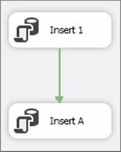
FIGURE 15-20

This package is quite basic in that all it does is insert some data into the table and then the last task will deliberately fail. Open SSMS and run the following code on the AdventureWorksDW database:

CREATE TABLE dbo.T1(col1 int)

In the Execute SQL Task named “Insert 1”, use the following code in the SQLStatement property to insert data into the table you just created:

INSERT dbo.T1(col1) VALUES(1)

To make the final task fail at runtime, use the following code in the SQLStatement property of the Execute SQL Task names “Insert A”:

INSERT dbo.T1(col1) VALUES("A")

Run the package with no transactions in place and see what happens. The results should look like Figure 15-21: The first task succeeds, and the second fails.

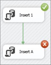
FIGURE 15-21

If you go to your database, you should see data inserted, as shown in Figure 15-22.

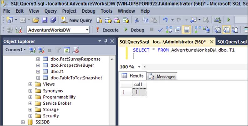
FIGURE 15-22

Now run the following code in SSMS to delete the data from the table:

TRUNCATE TABLE dbo.T1

Next, you want to set up the package to start a transaction that the tasks can join. You do that by setting the properties of the package, as shown in Figure 15-23. Set the TransactionOption property to Required.

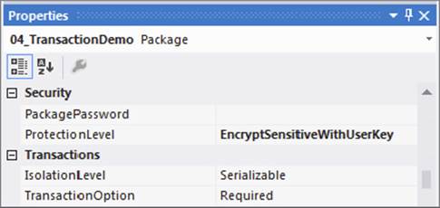
FIGURE 15-23

You now need to tell the tasks in the package to join this transaction, by setting their TransactionOption properties to Supported, as shown in Figure 15-24.

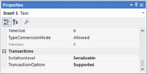
FIGURE 15-24

NOTE To quickly set the properties for all these tasks at once, select them by holding down the Ctrl key and clicking on each task, and set the TransactionOption property to the desired value.

Now when you re-execute the package, a DTC transaction will be started by the package, all the tasks will join, and because of the failure in the last task, the work in the package will be undone. Go back to SSMS and query the table. You should see no data in it. A good way to see the DTC transaction that was started is to look at the output window in SSIS:

SSIS package "C:\ProSSIS\Code\Ch15\04_TransactionDemo.dtsx" starting.

Information: 0x4001100A at 04_TransactionDemo: Starting distributed transaction for this container.

Error: 0xC002F210 at Insert A, Execute SQL Task: Executing the query "INSERT dbo.T1(col1) VALUES("A")" failed with the following error: "Invalid column name 'A'.". Possible failure reasons: Problems with the query, "ResultSet" property not set correctly, parameters not set correctly, or connection not established correctly.

Task failed: Insert A

Information: 0x4001100C at Insert A: Aborting the current distributed transaction.

Warning: 0x80019002 at 04_TransactionDemo: SSIS Warning Code

DTS_W_MAXIMUMERRORCOUNTREACHED. The Execution method succeeded, but the number of errors raised (1) reached the maximum allowed (1); resulting in failure. This occurs when the number of errors reaches the number specified in MaximumErrorCount. Change the MaximumErrorCount or fix the errors.

Information: 0x4001100C at 04_TransactionDemo: Aborting the current distributed transaction.

SSIS package "C:\ProSSIS\Code\Ch15\04_TransactionDemo.dtsx" finished: Failure.

Single Package, Multiple Transactions

The goal of this second package is to have two transactions running in the same package at the same time. Create the package as shown in Figure 15-25. If you’re not feeling creative, you can use the same statements in the tasks that you used in the previous example.

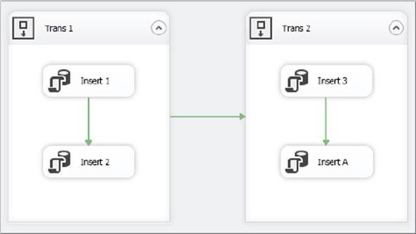
FIGURE 15-25

The package contains two Sequence Containers, each containing its own child tasks. The Trans 1 Container begins a transaction, and the child tasks join the transaction. The Trans 2 Container also starts a transaction of its own, and its child task joins that transaction. As you can see, the task in Trans 2 will deliberately fail. A real-world purpose of this scenario could be the logical loading of different sets of data. This could be useful when you have logical grouping of data manipulation routines to perform, and either all succeed or none of them succeed. The following table shows the tasks and containers in the package, along with the package itself and the setting of their TransactionOption property.

After you execute the package, the results should look like Figure 15-26. The first container succeeded, but the second one failed because its child task failed.

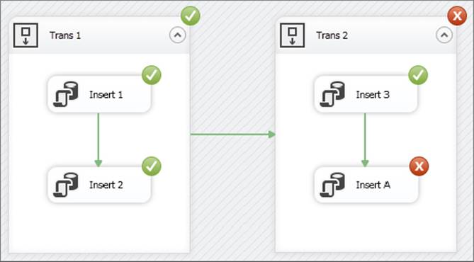
FIGURE 15-26

If you now look in the database, you will see that the numbers 1 and 2 were inserted. To prove that two transactions were instantiated, take another look at the output window:

SSIS package "C:\ProSSIS\Code\Ch15\05_MultipleTransactionDemo.dtsx" starting.

Information: 0x4001100A at Trans 1: Starting distributed transaction for this container.

Information: 0x4001100B at Trans 1: Committing distributed transaction started by this container.

Information: 0x4001100A at Trans 2: Starting distributed transaction for this container.

Error: 0xC002F210 at Insert A, Execute SQL Task: Executing the query "INSERT dbo.T1(col1) VALUES("A") " failed with the following error: "Invalid column name 'A'.". Possible failure reasons: Problems with the query, "ResultSet" property not set correctly, parameters not set correctly, or connection not established correctly.

Task failed: Insert A

Information: 0x4001100C at Insert A: Aborting the current distributed transaction.

Warning: 0x80019002 at Trans 2: SSIS Warning Code DTS_W_MAXIMUMERRORCOUNTREACHED. The Execution method succeeded, but the number of errors raised (1) reached the maximum allowed (1); resulting in failure. This occurs when the number of errors reaches the number specified in MaximumErrorCount. Change the MaximumErrorCount or fix the errors.

Information: 0x4001100C at Trans 2: Aborting the current distributed transaction.

Warning: 0x80019002 at 05_MultipleTransactionDemo: SSIS Warning Code DTS_W_MAXIMUMERRORCOUNTREACHED. The Execution method succeeded, but the number of errors raised (1) reached the maximum allowed (1); resulting in failure. This occurs when the number of errors reaches the number specified in MaximumErrorCount. Change the MaximumErrorCount or fix the errors.

SSIS package "C:\ProSSIS\Code\Ch15\05_MultipleTransactionDemo.dtsx" finished: Failure.

Two Packages, One Transaction

The third package in this series will highlight a transaction that spans multiple packages. Specifically, there will be two packages: “TransactionParent” and “TransactionChild.” The TransactionParent package will insert two rows into a table and then call the TransactionChild package using an Execute Package Task, which itself will insert two rows into the same table. You will then introduce an error in the TransactionParent package that causes it to fail. As a result, the work done in both packages is undone. Figure 15-27shows the TransactionParent package, and Figure 15-28 shows the TransactionChild package.

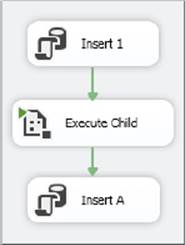
FIGURE 15-27

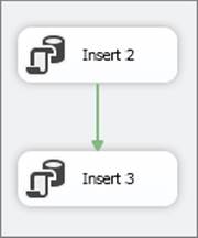
FIGURE 15-28

As in the previous example, you need to set the TransactionOption property on the tasks and containers. Use the values in the following table:

The point to note here is that the TransactionChild package becomes nothing more than another task. The parent of the TransactionChild package is the Execute Package Task in the TransactionParent package. Because the Execute Package Task is in a transaction, and the TransactionChild package also has its TransactionOption set to Supported, it will join the transaction in the TransactionParent package.

If you change the TransactionOption property on the Execute Package Task in the TransactionParent package to Not Supported (refer to Figure 15-24), when the final task in the TransactionParent package fails, the work in the TransactionChild package will not be undone.

Single Package Using a Native Transaction in SQL Server

This example differs from the others in that you are going to use the transaction-handling abilities of SQL Server and not those of MS DTC. Although the example is short, it does demonstrate that transactions can be used in packages that are not MS DTC transactions. Native SQL transactions provide you with a finer level of granularity when deciding what data is rolled back and committed, but they are possible only with SQL Server. The package for this example is shown in Figure 15-29.

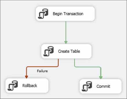
FIGURE 15-29

Although you cannot see it because the screenshot is black and white, the workflow line from the Create Table Transactions Task to the Rollback Task is red, indicating failure; however, you can see the word failure next to the precedence constraint line.

The following table lists the contents of the SQLStatement property for each of the Execute SQL Tasks:

The key to making the package use the native transaction capabilities in SQL Server is to have all the tasks use the same Connection Manager. In addition, you must ensure that the RetainSameConnection property on the Connection Manager is set to True, as shown in Figure 15-30.

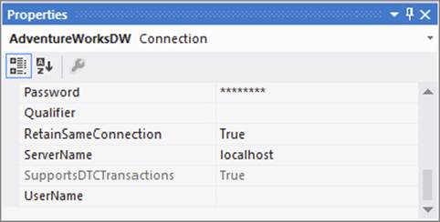
FIGURE 15-30

When the package is executed, SQL Server will fire up a transaction and either commit or rollback that transaction at the end of the package.

Now have a look at that happening on SQL Server by using Profiler, as shown in Figure 15-31. Profiler is very useful in situations like this. Here you simply want to confirm that a transaction was started and that it either finished successfully or failed. You can also use Profiler when firing SSIS packages to ensure that what you assume you are executing is what you are actually executing. Explaining how to use SQL Server Profiler is beyond the scope of this book, and more information can be found in SQL Server Books Online.

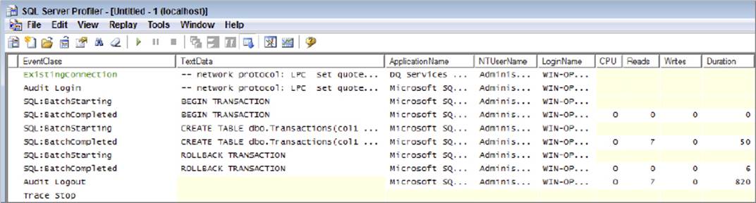
FIGURE 15-31

That ends your whistle-stop look at transactions within SSIS packages. Next, it’s time to look at error outputs and how they can help with scalability.

ERROR OUTPUTS

Error outputs can obviously be used to improve reliability, but they also have an important part to play in terms of scalability as well. From a reliability perspective, they are a critical feature for coping with bad data. An appropriately configured component will direct failing rows down the error output, rather than the main output. After being removed from the main Data Flow path, these rows may receive additional treatment and cleansing to enable them to be recovered and merged back into the main flow. They can be merged explicitly, such as with a Union All Transformation, or implicitly through a second adapter directed at the final destination. Alternatively, they could be discarded. Be careful of discarding rows entirely; you may find out you need them later! More often, rows on the error output are logged and dealt with later.

WARNING The error outputs are not always accurate in removing just the bad rows. In the scenario of using delimited flat files as a source, you may have rows missing delimiters. This can cause havoc with the data written to the error output and the expected good data.

The capability to recover rows is perhaps the most useful course of action. If a data item is missing in the source extract but required in the final destination, the error flow path can be used to fix this. If the data item is available from a secondary system, then a lookup could be used. If the data item is not available elsewhere, then perhaps a default value could be used instead.

In other situations, the data may be out of range for the process or destination. If the data causes an integrity violation, then the failed data could be used to populate the constraining reference with new values, and then the data itself could be successfully processed. If a data type conflict occurs, then maybe a simple truncation would suffice, or an additional set of logic could be applied to try to detect the real value, such as with data time values held in strings. The data could then be converted into the required format.

When assumptions or fixes have been made to data in this way, it is best practice to always mark rows as having been manipulated; that way, if additional information becomes available later, they can be targeted directly. In addition, whenever an assumption is made, it should be clearly identified as such to the end user.

All the scenarios described here revolve around trying to recover from poor data, within the pipeline and the current session, allowing processing to continue, and ideally fixing the problem such that data is recovered. This is a new concept compared with DTS and several other products, but the ability to fix errors in real time is a very valuable option that you should always consider when building solutions.

The obvious question that then occurs is this: Why not include the additional transformations used to correct and cleanse the data in the main Data Flow path, so that any problems are dealt with before they cause an error? This would mean that all data flows down a single path, and the overall Data Flow design may be simpler, with no branching and merging flows. This is where the scalability factor should enter into your solution design. Ideally, you want to build the simplest Data Flow Task possible, using as few transformations as possible. The less work you perform, the greater the performance and therefore scalability.

Figure 15-32 illustrates a Data Flow Task used to load some data. In this contrived scenario, some of the rows will be missing values for SpecialtyCode and ConsultantCode. The source data contains text descriptions as well, so these are being used to perform a lookup to retrieve the missing values. The initial design logic specifies evaluating the column for NULL values in a Conditional Split Transformation. Bad rows are directed to an alternate output that connects to the Lookup Transformation. Once the lookup has populated the missing value, the rows are then fed back into the main pipeline through the Union All Transformation. The same pattern is followed for the SpecialtyCode and ConsultantCode columns, ensuring that the final insert through the OLE DB Destination has all good data. This is the base design for solving your problem, and it follows the procedural logic quite closely.

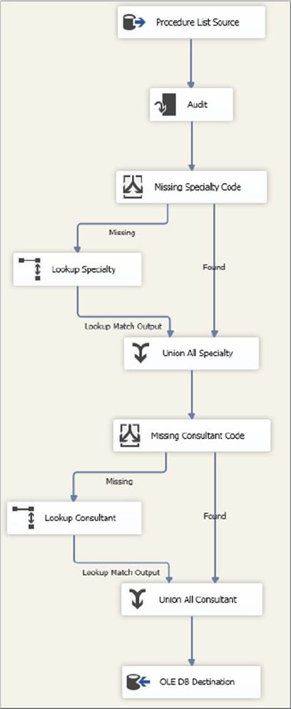
FIGURE 15-32

Figure 15-33 shows two alternative Data Flow Task designs, presented side by side for easy comparison. In the first design, you disregard any existing data in the SpecialtyCode and ConsultantCode columns and populate them entirely through the lookup. Although this may seem like wasted effort, the overall design is simpler, and in testing it was slightly faster compared to the more complicated design in Figure 15-32. This example used a test data set that had a bad row ratio of 1 in 3 — that is, one row in three had missing values. If the ratio dropped to 1 in 6 for the bad rows, then the two methods performed the same.

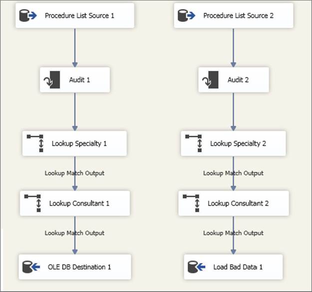
FIGURE 15-33

The second design assumes that all data is good until proven otherwise, so you insert directly into the destination. Rows that fail because of the missing values pass down the error output, “OLE DB Destination Error Output,” and are then processed through the two lookups. The choice between the two designs is whether you fix all rows or only those that fail. Using the 1 in 3 bad rows test data, fixing only the failed rows was 20 percent faster than fixing all rows. When the bad row ratio dropped to 1 in 6, the performance gain also dropped, to only 10 percent.

As demonstrated by the preceding examples, the decision regarding where to include the corrective transformations is based on the ratio of good rows to bad rows, as compared to how much work is required to validate the quality of the data. The cost of fixing the data should be excluded if possible, as that is required regardless of the design, but often the two are inseparable.

The performance characteristics of the corrective transformations should also be considered. In the preceding examples, you used lookups, which are inherently expensive transformations. The test data and lookup reference data included only six distinct values to minimize the impact on overall testing. Lookups with more distinct values, and higher cardinality, will be more expensive, as the caching becomes less effective and itself consumes more resources. The cache modes are discussed in Chapter 7 of this book.

In summary, the more expensive the verification, the more bad rows you require to justify adding the validation and fix to the main flow. For fewer bad rows, or a more expensive validation procedure, you have increased justification for keeping the main flow simple and for using the error flow to perform the corrective work.

The overall number of rows should also influence your design, because any advantages or disadvantages are amplified with a greater number of rows, regardless of the ratio. For a smaller number of rows, the fixed costs may outweigh the implied benefits, as any component has a cost to manage at runtime, so a more complicated Data Flow Task may not be worthwhile with fewer overall rows.

This concept of using error flows versus the main flow to correct data quality issues and related errors is not confined to those outputs that implement the error output explicitly. You can apply the same logic manually, primarily through the use of the Conditional Split Transformation, as shown in the first example (refer to Figure 15-32). You can perform a simple test to detect any potential issues, and direct rows of differing quality down different outputs. Where expensive operations are required, your goal is to ensure that as few rows as possible follow this path and that the majority of the rows follow cheaper, and usually simpler, routes to their destination.

Finally, don’t be put off by the term error output; it isn’t something to be avoided at all costs. Component developers often take advantage of the rich underlying pipeline architecture, using error outputs as a simple way of indicating the result of a transformation for a given row. They don’t affect the overall success or failure state of a package, so don’t be put off from using them.

Of course, the performance figures quoted here are for demonstration purposes only. They illustrate the differences between the methods described, but they should not be taken as literal values that you can expect to reproduce, unless you’re using exactly the same design, data, and environment. The key point is that testing such scenarios should be a routine part of your development practice.

SCALING OUT

You are no doubt already familiar with the term scaling out, and of course the concept can be applied to SSIS systems. Although there are no magical switches here, SSIS offers several interesting features, and in this section you will see how they can be applied and how they can benefit reliability as well.

Architectural Features

There are two important architectural features in Integration Services that give the tool great capabilities. The first feature is the Lookup Transformation. The second feature is the data pipeline itself. These features give SSIS the abilities to move and compare data in a very fast and efficient manner.

Lookup Transformation

The Lookup Transformation has the ability to cache data, and it has several options available to optimize that configuration. The Cache Data Sources available to this transformation include pure in-memory cache and persistent file storage (also called persisted cache). Both of these options require the transformation to be configured to use the full-cache option, however. A Connection Manager called the Cache Connection Manager governs these two types of caching options.

Caching operations in the Lookup Transformation provide three modes to choose from: full, partial, or none. Using the full-cache mode, the lookup set will be stored in its entirety and will load before the lookup operation actually runs, but it will not repopulate on every subsequent lookup operation. A partial cache stores only matched lookups, and no-cache will repopulate the cache every time. Of course, you can also manually configure the size of the cache to store, measured in megabytes.

Persistent file storage is another very exciting caching feature, as it will store your cache in a file that can be reused across other packages. Talk about reusability! To add to the benefit, the cache can be loaded from a variety of sources, including text files, XML files, or even web services. Lastly, partial-cache mode has a cache option called miss-cache, in which items being processed for lookup that do not have a match will be cached, so they will not be retried in future lookup operations. All these features translate into scalability and performance gains.

Data Pipeline

The data pipeline is the workhorse of the data processing engine. The data pipeline architecture is able to provide a fully multi-threaded engine for true parallelism. This allows most pipelines to scale out well without a lot of manual tweaking.

Scaling Out Memory Pressures

By design, pipeline processing takes place almost exclusively in memory. This enable faster data movement and transformations, and a design goal should always include making a single pass over your data. This eliminates time-consuming staging and the costs of reading and writing the same data several times. The potential disadvantage of this is that for large amounts of data and complicated sets of transformations, you need a large amount of memory, and it needs to be the right type of memory for optimum performance.

The virtual memory space for 32-bit Windows operating systems is limited to 2GB by default. Although you can increase this amount through the use of the /3GB switch applied in the boot.ini file, this often falls short of the total memory currently available. This limit is applied per process, which for your purposes means a single package during execution. Therefore, by partitioning a process across multiple packages, you can ensure that each of the smaller packages is its own process, thereby taking advantage of the full 2–3GB virtual space independently. The most common method of chaining packages together to form a consolidated process is through the Execute Package Task, in which case it is imperative that you set the Child package to execute out of process. To enable this behavior, you must set the ExecuteOutOfProcess property to true.

Note that unlike the SQL Server database engine, SSIS does not support Advanced Windowing Extensions (AWE), so scaling out to multiple packages across processes is the only way to take advantage of larger amounts of memory. If you have a very large memory requirement, then you should consider a 64-bit system for hosting these processes. Whereas just a few years ago it would have been very expensive and hard to find software and drivers for all your needs, 64-bit systems are now common for enterprise hardware and should be considered for any business database.

For a more detailed explanation of how SSIS uses memory, and the in-memory buffer structure used to move data through the pipeline, see Chapter 16.

Scaling Out by Staging Data

The staging of data is very much on the decline; after all, why incur the cost of writing to and reading from a staging area when you can perform all the processing in memory with a single pass of data? With the inclusion of the Dimension and Partition Processing Destinations, you no longer need a physical Data Source to populate your SQL Server Analysis Services (SSAS) cubes — yet another reason for the decline of staging or even the traditional data warehouse. Although this is still a contentious debate, the issue here is this: Should you use staging during the SSIS processing flow? Although it may not be technically required to achieve the overall goal, there are still certain scenarios when you may want to, for both scalability and reliability reasons.

For this discussion, staging could also be described as partitioning. Although the process can be implemented within a single Data Flow Task, for one or more of the reasons described next, it may be subdivided into multiple Data Flow Tasks. These smaller units could be within a single package, or they might be distributed through several, as discussed next. The staged data will be used only by another Data Flow Task and does not need to be accessed directly through regular interfaces. For this reason, the ideal choices for the source and destinations are the raw file adapters. This could be described as vertical partitioning, but you could also overlay a level of horizontal partitioning, by executing multiple instances of a package in parallel.

Raw file adapters enable you to persist the native buffer structures to disk. The in-memory buffer structure is simply dumped to and from the file, without any translation or processing as found in all other adapters, making these the fastest adapters for staging data. You can take advantage of this to artificially force a memory checkpoint to be written to disk, thereby enabling you to span multiple Data Flow Tasks and packages. Staging environments and raw files are also discussed in Chapter 16, but some specific examples are illustrated here.

The key use for raw files is that by splitting one Data Flow Task into at least two individual Data Flow Tasks, the primary task can end with a raw file destination and the secondary task can begin with a raw file source. The buffer structure is exactly the same between the two tasks, so the split is basically irrelevant from an overall flow perspective, but it provides perfect preservation of the two tasks.

Data Flow Restart

As covered previously in this chapter, the checkpoint feature provides the capability to restart a package from the point of failure, but it does not extend inside a Data Flow Task. However, if you divide a Data Flow Task into one or more individual tasks, each linked together by raw files, you immediately gain the capability to restart the combined flow. Through the correct use of native checkpoints at the (Data Flow) task level, this process becomes very simple to manage.

Deciding where to divide a flow is subjective, but two common choices are immediately after extraction and immediately after transformation, prior to load. The post-extraction point offers several key benefits, including performance, meeting source system service level agreements (SLAs), and consistency. Many source systems are remote, so extraction might take place over suboptimal network links, and it can be the slowest part of the process. By staging immediately after the extraction, you don’t have to repeat this slow step in the event of a failure and restart. There may also be an impact on the source system during the extraction, which often takes place during a specified time window when utilization is low. In this case, it may be unacceptable to repeat the extract in the event of a failure until the next time window, usually the following night. Finally, the initial extraction will take place at a more consistent time each night, which could provide a better base for tracking history. Staging post-transformation simply ensures that the transformation is not wasted if the destination system is unavailable. If the transformations are time intensive, this cost-savings can really add up!

You may wish to include additional staging points mid-transformation. These would usually be located after particularly expensive operations and before those that you suspect are at risk to fail. Although you can plan for problems, and the use of error outputs described previously should enable you to handle many situations, you can still expect the unexpected and plan a staging point with this in mind. The goal remains the same — the ability to restart as close to the failure point as possible and to reduce the cost of any reprocessing required.

Figure 15-34 shows an example data load process that you may wish to partition into multiple tasks to take advantage of Data Flow restart.

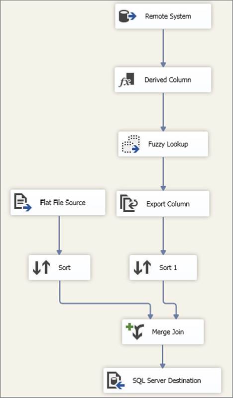
FIGURE 15-34

For this scenario, the OLE DB Source Component connects to a remote SQL Server over a slow network link. Because of the time taken for this data extraction and the impact on the source system, it is not acceptable to repeat the extract if the subsequent processing fails for any reason. Therefore, you choose to stage data through a raw file immediately after the Source Component. The resulting Data Flow Task layout is shown in Figure 15-35.

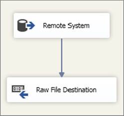
FIGURE 15-35

The Flat File Source data is accessed across the LAN, and it needs to be captured before it is overwritten. The sort operation is also particularly expensive because of the volume of data. For this reason, you choose to stage the data after the sort is complete. The resulting Data Flow Task is shown in Figure 15-36.

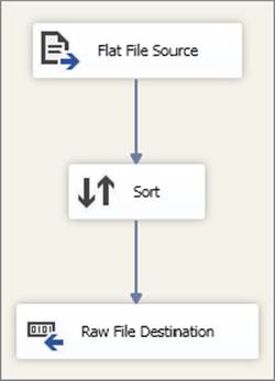
FIGURE 15-36

Finally, you use a third Data Flow Task to consume the two staging raw files and complete the process, as shown in Figure 15-37.

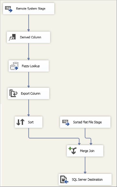
FIGURE 15-37

Following this example, a single Data Flow Task has been divided into three separate tasks. For the purpose of restarting a failed process, you would use a single package and implement checkpoints on each of the three Data Flow Tasks.

Scaling across Machines

In a similar manner to the Data Flow restart just discussed, you can also use raw file adapters to partition the Data Flow Task. By separating tasks into different packages, you can run packages across machines. This may be advantageous if a specific machine has properties not shared with others. Perhaps the machine capable of performing the extract is situated in a different network segment from the machine best suited for processing the data, and direct access is unavailable between the main processing machine and the source. The extract could be performed, and the main processing machine would then retrieve the raw data to continue the process. These situations are organizational restrictions, rather than decisions driven by the design architecture.

Another method for scaling across machines is to use horizontal partitioning. A simple scenario would utilize two packages. The first package would extract data from the source system, and through the Conditional Split you produce two or more exclusive subsets of the data and write this to individual raw files. Each raw file would contain some of the rows from the extract, as determined by the expression used in the Conditional Split. The most common horizontal partition scheme is time-based, but any method could be used here. The goal is to subdivide the total extract into manageable chunks; so, for example, if a sequential row number is already available in the source, this would be ideal, or one could be applied (see the T-SQL ROW_NUMBER function). Similarly a Row Number Transformation could be used to apply the numbering, which could then be used by the split, or the numbering and splitting could be delivered through a Script Component.

With a sorted data set, each raw file may be written in sequence, completing in order, before moving on to the next one. While this may seem uneven and inefficient, it is assumed that the time delay between completion of the first and final destinations is inconsequential compared to the savings achieved by the subsequent parallel processing.

Once the partitioned raw files are complete, they are consumed by the second package, which performs the transformation and load aspects of the processing. Each file is processed by an instance of the package running on a separate machine. This way, you can scale across machines and perform expensive transformations in parallel. For a smaller-scale implementation, where the previously described 32-bit virtual memory constraints apply, you could parallel process on a single machine, such that each package instance would be a separate thread, with its own allocation of virtual memory space.

For destinations that are partitioned themselves, such as a SQL Server data warehouse with table partitions or a partitioned view model, or Analysis Services partitions, it may also make sense to match the partition schema to that of the destination, such that each package addresses a single table or partition.

Figure 15-38 shows a sample package that for the purposes of this example you will partition horizontally.

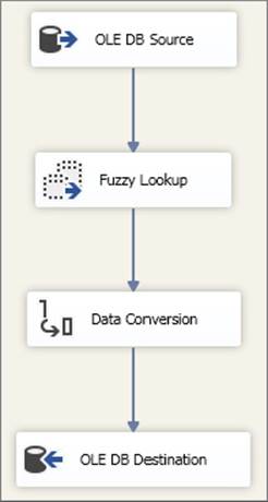
FIGURE 15-38

In this scenario, the Fuzzy Lookup is processing names against a very large reference set, and this is taking too long. To introduce some parallel processing, you decide to partition on the first letter of a name field. It is deemed stable enough for matches to be within the same letter, although in a real-world scenario this may not always be true. You use a Conditional Split Transformation to produce the two raw files partitioned from A to M and from N to Z. This primer package is illustrated in Figure 15-39.

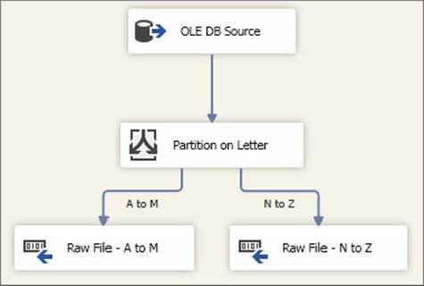
FIGURE 15-39

Ideally, you would then have two instances of the second package (Figure 15-40) running in parallel on two separate machines. However, you need to ensure that the lookup data is filtered on name to match the raw file. Not all pipeline component properties are exposed as expressions, allowing you to dynamically control them, so you would need two versions of the package, identical except for a different Reference table name property in the Fuzzy Lookup, also shown in Figure 15-40. In preparation, you would create two views, one for names A to M and the other for names N to Z, to match the two raw files. The two package versions would each use the view to match the raw file they will process.

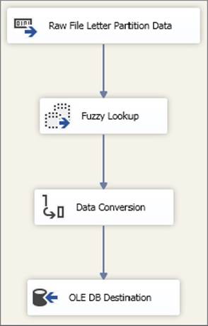
FIGURE 15-40

For any design that uses raw files, the additional I/O cost must be evaluated against the processing performance gains, but for large-scale implementations it offers a convenient way of ensuring consistency within the overall flow and doesn’t incur the translation penalty associated with other storage formats.

Scaling Out with Parallel Loading

You have seen several ways to scale out SSIS in this chapter. Now you will learn how to scale out using parallelization with the data loads. You can accomplish faster load times by loading multiple partitions at once using SSIS from either a staging environment or multiple files of sorted data. If the data resides in a flat file, you may want to consider loading those files into a staging table so the data can be pre-sorted.

The first item you will need is a control table. This will tell the SSIS packages which data to pull for each partition in the destination. The control table will contain a list of data that needs to be checked out. The following code will create this table:

USE [AdventureWorksDW]

GO

CREATE TABLE [dbo].[ctlTaskQueue](

[TaskQueueID] [smallint] IDENTITY(1,1) NOT NULL,

[PartitionWhere] [varchar](20) NOT NULL,

[Priority] [tinyint] NOT NULL,

[StartDate] [datetime] NULL,

[CompleteDate] [datetime] NULL,

CONSTRAINT [PK_ctlTaskQueue] PRIMARY KEY CLUSTERED

(

[TaskQueueID] ASC

)WITH (PAD_INDEX = OFF, STATISTICS_NORECOMPUTE = OFF, IGNORE_DUP_KEY = OFF,

ALLOW_ROW_LOCKS = ON, ALLOW_PAGE_LOCKS = ON) ON [PRIMARY])

The PartitionWhere column is the data used to divide the data up into parallel loading. This will be a part of the WHERE clause that queries from the source of the staging table conditionally. For example, Figure 15-41 shows you a table that’s ready to be used. Each WHEREclause should ideally align with a partition on your destination table. The StartDate and CompleteDate columns show you when the work was checked out and completed.

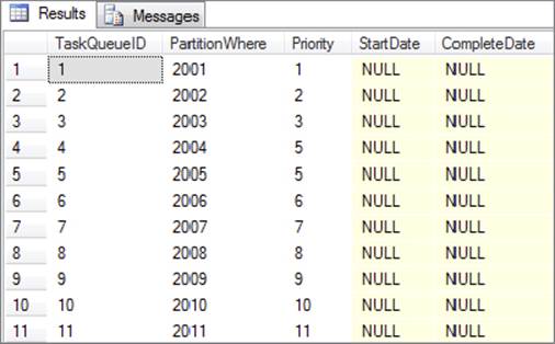
FIGURE 15-41

Run the following code to populate these values:

USE [AdventureWorksDW]

GO

INSERT INTO [dbo].[ctlTaskQueue]

([PartitionWhere]

,[Priority]

,[StartDate]

,[CompleteDate])

VALUES

(2001,1, null, null),

(2002,2, null, null),

(2003,3, null, null),

(2004,4, null, null),

(2005,5, null, null),

(2006,6, null, null),

(2007,7, null, null),

(2008,8, null, null),

(2009,9, null, null),

(2010,10, null, null),

(2011,11, null, null)

GO

Now create an SSIS package named ParallelDemo.dtsx that will perform the parallel load. This section will show you the basics for creating a package to perform a parallel load. You will still need to apply best practices to this package afterward, for example, additional elements like package checkpoints, parameters, and a master package to run all of your parallel loads. Create three SSIS variables in the package, as shown in Figure 15-42. Don’t worry about the value of the strSQLStatement variable, as you will modify it later to use an expression.

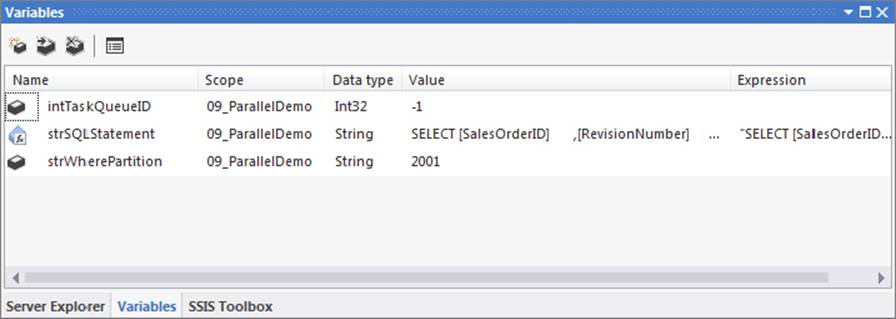
FIGURE 15-42

Next drag in a For Loop Container, which will be used to look for new work in the control table you just created. Configure the container to use the intTaskQueueID variable, as shown in Figure 15-43. The loop will repeat while intTaskQueueID is not 0. The tasks inside the loop will be responsible for setting the variable to 0 once the work is complete.

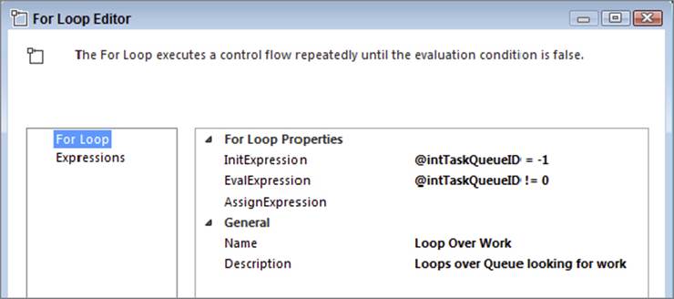
FIGURE 15-43

Next you will run the following code to create a stored procedure that will check out the work to be done. The stored procedure is going to output two variables: one for the task that needs to be worked on (@TaskQueueID) and the filter that will be applied on the source table (@PartitionWhere). After the task is read, it also checks the work out by updating the StartDate column.

USE [AdventureWorksDW]

GO

CREATE PROCEDURE [dbo].[ctl_UseTask]

@TaskQueueID int OUTPUT,

@PartitionWhere varchar(50) OUTPUT

AS

SELECT TOP 1

@TaskQueueID = TaskQueueID,

@PartitionWhere = PartitionWhere

from ctlTaskQueue

WHERE StartDate is NULL

AND CompleteDate is NULL

ORDER BY Priority asc

IF @TaskQueueID IS NULL

BEGIN

SET @TaskQueueID = 0

END

ELSE

BEGIN

UPDATE ctlTaskQueue

SET StartDate = GETDATE()

WHERE TaskQueueID = @TaskQueueID

END

GO

Drag an Execute SQL Task into the For Loop Container and configure it to match Figure 15-44, using the following code in the SQLStatement. This will execute the stored procedure and get the task queue and the WHERE clause values from the table. You could also have altered the stored procedure to have an input variable of what queue you’d like to read from.

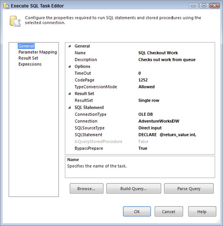
FIGURE 15-44

DECLARE @return_value int,

@TaskQueueID int,

@PartitionWhere varchar(50)

EXEC @return_value = [dbo].[ctl_UseTask]

@TaskQueueID = @TaskQueueID OUTPUT,

@PartitionWhere = @PartitionWhere OUTPUT

SELECT convert(int,@TaskQueueID) as N'@TaskQueueID',

@PartitionWhere as N'@PartitionWhere'

GO

Open the Result Set window in the Execute SQL Task and configure it to match Figure 15-45. Each value maps to a variable in SSIS. The Result Name of 0 means the first column returned, and the columns are sequentially numbered from there.

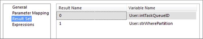
FIGURE 15-45

Now you will set the variable strSQLStatement to be dynamic by adding the following code to the Expression property in the strSQLStatement variable. This strSQLStatement variable will be used as your OLE DB Source Component in the Data Flow Task you will create in a moment. This query could be whatever you’d like. In this example, you are gathering data out of a Transactions table between a given date range. The strWherePartition is populated from the previous Execute SQL Task, and the date range should match your target table’s partition layout. The ORDER BY clause is going to pre-sort the data on the way out. Ideally this column would have a clustered index on it to make the sort more efficient.

"SELECT [SalesOrderID]

,[RevisionNumber]

,[OrderDate]

,[DueDate]

,[ShipDate]

,[Status]

,[OnlineOrderFlag]

,[SalesOrderNumber]

,[PurchaseOrderNumber]

,[AccountNumber]

,[CustomerID]

,[SalesPersonID]

,[TerritoryID]

,[BillToAddressID]

,[ShipToAddressID]

,[ShipMethodID]

,[CreditCardID]

,[CreditCardApprovalCode]

,[CurrencyRateID]

,[SubTotal]

,[TaxAmt]

,[Freight]

,[TotalDue]

,[Comment]

,[rowguid]

,[ModifiedDate]

FROM [AdventureWorks].[Sales].[SalesOrderHeader]

WHERE [ShipDate] > '"+ @[User::strWherePartition] + "-01-01' and

[ShipDate] <= '" + @[User::strWherePartition] + "-12-31' ORDER BY [ShipDate] "

Now you are ready to create the Data Flow Task. Drag a Data Flow Task over and connect it to the Execute SQL Task inside the loop. In the Data Flow tab, drag an OLE DB Source Component over and connect it to your source connection manager and use thestrSQLStatement variable as your source query, as seen in Figure 15-46.

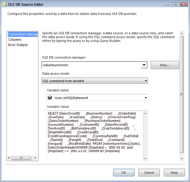
FIGURE 15-46

You can connect the OLE DB Source Component to any other component you’d like for this example, such as a Union All Transformation. You are using a Union All Transformation as a temporary dead-end destination so you can see the number of rows that flow down that part of the Data Flow path. You can also use a Data Viewer before the Union All Transformation to see the data in those rows. Ideally though, you should connect the source to any business logic that you may have and then finally into a destination. Your ultimate destination should ensure that the data is committed into a single batch. Otherwise, fragmentation may occur. You can do this by ensuring that the destination’s “Max Insert Commit Size” is a high number, well above the number of rows that you expect (though in some cases you may not know this number). Keep in mind that the source query partition should have already sorted the data and be a small enough chunk of data to not cause major impact to the transaction log in SQL Server.

Back in the Control Flow, you’ll want to add conditional logic between the Execute SQL Task and the Data Flow Task to execute the Data Flow Task only if more work is pending. To do this, double-click on the green precedence constraint connecting the two tasks and change the Evaluation operation property to be Expression and Constraint. Then, set the expression to @intTaskQueueID > 0, as seen in Figure 15-47.

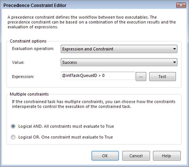
FIGURE 15-47

The final step is to update the queue table to say the work is complete. You can do this by connecting an Execute SQL Task to the Data Flow Task. This task should update the ctlTaskQueue table in the AdventureWorksDW database to show the CompleteDate to the current time. This can be done in the following query or stored procedure:

UPDATE ctlTaskQueue

SET CompleteDate = GETDATE()

WHERE TaskQueueID = ?

The question mark in the previous code will be mapped to the intTaskQueueID variable in the Parameter Mapping tab in the Execute SQL Task. The final Control Flow of the package should look like Figure 15-48.

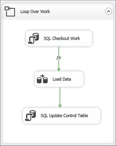
FIGURE 15-48

With the plumbing done, you’re now ready to create parallelism in your package. One way of accomplishing this is through a batch file. The following batch file will perform this with the START command. Optionally, you can reset your tables through the SQLCMD executable, as shown here as well. The batch file will execute DTEXEC.exe N number of times in parallel and work on independent workloads. Where you see the SQLCMD command, you may also want to ensure that the trace flags are on if they’re not on already.

@Echo off

sqlcmd -E -S localhost -d AdventureWorksDW -Q "update dbo.ctlTaskQueue set StartDate = NULL, CompleteDate = NULL"

FOR /L %%i IN (1, 1, %1) DO (

ECHO Spawning thread %%i

START "Worker%%i" /Min "C:\Program Files\Microsoft SQL Server\120\DTS\Binn\DTEXEC.exe" /FILE "C:\ProSSIS\Code\Ch15\09_ParallelDemo.dtsx" /CHECKPOINTING OFF /REPORTING E

)

The %1 in the preceding code represents the N variable that is passed in. To use the batch file, use the following command, where 5 represents the number of DTEXEC.exe commands that you wish to run in parallel. Save this file as ParallelBatch.cmd. You can do this from Notepad. Then, run the batch file with the following code in a command window.

ParallelBatch.cmd 5

As each worker thread spins up, it will log its number. The results will look like Figure 15-49.

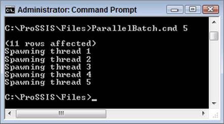
FIGURE 15-49

WARNING Beware of executing packages from the command line. Even though executing packages from the command line can seem like an easy way to achieve parallelism and scalability, the execution functionality is limited. Using the DTEXEC.exe command will only work with Legacy Package Model features. If you want to take advantage of the latest Project Model features, you will need to utilize an alternative method.

One final note about parallelism is that if you load data using multiple cores into a target table, it will cause fragmentation in the target table. Each core would handle sorting its individual chunk of data that it’s responsible for; then when each chunk of data is pieced together, data may be inserted into different pages. One way to prevent that is to ensure that each thread of DTEXEC.exe connects to a different TCP/IP port and in soft NUMA node. With soft NUMA, you can bind any port or IP address to a given CPU core. By doing this, each SQL Server Destination in the Data Flow Task would always use only one CPU in SQL Server. It essentially allows SSIS and the SQL Server Destination to mimic MAXDOP 1 in T-SQL.

There is more setup needed to create the soft NUMA node. A complete soft NUMA explanation is beyond the scope of this book, and you can learn more on SQL Server Books Online. The following steps will point you in the right direction to getting soft NUMA working:

1. Create the soft NUMA node in the registry of the SQL Server instance, which isolates each node to a CPU core.

2. Bind the soft NUMA nodes to a given port in SQL Server Configuration Manager under Network Configuration.

3. Restart the SQL Server instance.

4. Change the package to bind the connection manager in the worker package to a different port by changing the ServerName property and adding the port following the server name (InstanceName, 1433, for example). You’ll want this port to be dynamically set through an expression and variable so the variable can be passed in through the calling batch file.

SUMMARY

In this chapter, you looked at some of the obvious SSIS features provided to help you build reliable and scalable solutions, such as checkpoints and transactions. You also learned some practices you can employ, such as Data Flow Task restarts and scaling across machines; although these may not be explicit features, they are nonetheless very powerful techniques that can be implemented in your package designs.