Professional Microsoft SQL Server 2014 Integration Services (Wrox Programmer to Programmer), 1st Edition (2014)
Chapter 16. Understanding and Tuning the Data Flow Engine
WHAT’S IN THIS CHAPTER?
· Understanding the Control Flow and Data Flow
· Learning the Data Flow architecture and transformation types
· Designing and tuning the Data Flow
· Troubleshooting Data Flow performance
WROX.COM DOWNLOADS FOR THIS CHAPTER
You can find the wrox.com code downloads for this chapter at www.wrox.com/go/prossis2014 on the Download Code tab.
This chapter focuses on how the Data Flow engine works, because as you seek to expand your knowledge and skills with SSIS, you will need to understand how to best leverage and tune your packages and Data Flows. The chapter begins with a consideration of the architecture of the engine and its components, and then describes best practices for design and optimization, including the following concepts:
· Control Flow and Data Flow comparison
· Data Flow Transformation types
· Data Flow buffer architecture and execution trees
· Data Flow execution monitoring
· Data Flow design practices
· Data Flow engine tuning
· Performance monitoring
The initial part of this chapter is more abstract and theoretical, but we’ll then move into the practical and tangible. In the concluding sections, you will apply the knowledge you have developed here, considering a methodology for optimization and looking at a few real-world scenarios.
Some of you will have worked with a previous edition of SSIS; for others, this will be your first time working with the tool. In many ways, each new version of SSIS has made improvements to the Data Flow architecture, adding more scalability and performance and fine-tuning the performance of the Data Flow engine.
For those of you with some knowledge of the SSIS pipeline architecture, two important features for the Data Flow engine are backpressure management and active component logging in the SSIS Server. These features provide scalability and advanced insight into the Data Flow. But let’s begin with the basics of the SSIS engine.
THE SSIS ENGINE
Before learning about buffers, asynchronous components, and execution trees, you might find it useful to consider this analogy — traffic management. While driving in a big city, have you ever wondered how the traffic system works? It’s remarkable how well coordinated the traffic lights are. In Manhattan, for example, a taxi ride can take you from midtown to downtown in minutes — in part because the lights are timed in a rolling fashion to maintain efficiency. The heavy fine assessed to anyone who “locks the box” (remains in the intersection after the light turns red) demonstrates how detrimental it is to interfere with the synchronization of such a complex traffic grid.
Contrast the efficiency of Manhattan with the gridlock and delays that result from a poorly designed traffic system. We have all been there before — sitting at a red light for minutes despite the absence of traffic on the intersecting streets, and then after the light changes, you find yourself in the same scenario at the next intersection! Even in a light-traffic environment, progress is impeded by poor coordination and inefficient design.
In the case of optimizing traffic patterns in a big city, good traffic management design focuses on easing congestion by keeping traffic moving or redirecting more highly congested areas to less utilized streets. A traffic jam occurs when something slows or blocks the flow of traffic. This causes backpressure behind the cause of the jam as cars queue up waiting to pass.
Bringing this back around to SSIS, in some ways the engine is similar to the grid management of a big city because the SSIS engine coordinates server resources and Data Flow for efficient information processing and management of data backpressure. Part of the process of making package execution efficient requires your involvement. In turn, this requires knowing how the SSIS engine works and some important particulars of components and properties that affect the data processing. That is the purpose of this chapter: to provide the groundwork for understanding SSIS, which will lead to better — that is, more efficient — design.
Understanding the SSIS Data Flow and Control Flow
From an architectural perspective, the difference between the Data Flow and Control Flow is important. One aspect that will help illustrate the distinction is to look at them from the perspective of how the components are handled. In the Control Flow, the task is the smallest unit of work, and a task requires completion (success, failure, or just completion) before subsequent tasks are handled. In the Data Flow, the transformation, source, and destination are the basic components; however, the Data Flow Components function very differently from a task. For example, instead of one transformation necessarily waiting for another transformation to complete before it can proceed with the next set of transformation logic, the components work together to process and manage data.
Comparing Data Flow and Control Flow
Although the Control Flow looks very similar to the Data Flow, with processing objects (tasks and transformations) and connectors that bridge them, there is a world of difference between them. The Control Flow, for example, does not manage or pass data between components; rather, it functions as a task coordinator with isolated units of work. Here are some of the Control Flow concepts:
· Workflow orchestration
· Process-oriented
· Serial or parallel tasks execution
· Synchronous processing
As highlighted, the Control Flow Tasks can be designed to execute both serially and in parallel — in fact, more often than not there will be aspects of both. A Control Flow Task can branch off into multiple tasks that are performed in parallel or as a single next step that is performed essentially in serial from the first. To show this, Figure 16-1 illustrates a very simple Control Flow process whose tasks are connected in a linear fashion. The execution of this package shows that the components are serialized — only a single task is executing at a time.
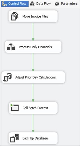
FIGURE 16-1
The Data Flow, conversely, can branch, split, and merge, providing parallel processing, but this concept is different from the Control Flow. Even though there may be a set of connected linear transformations, you cannot necessarily call the process a serial process, because the transformations in most cases will run at the same time, handling subsets of the data in parallel and passing groups of data downstream. Here are some of the unique aspects of the Data Flow:
· Information-oriented
· Data correlation and transformation
· Coordinated processing
· Streaming in nature
· Source extraction and destination loading
Similar to the Control Flow shown in Figure 16-2, Figure 16-2 also models a simple Data Flow whose components are connected one after the other. The difference between the Data Flow in Figure 16-2 and the Control Flow in Figure 16-2 is that only a single task is executing in the linear flow. In the Data Flow, however, all the transformations are doing work at the same time.
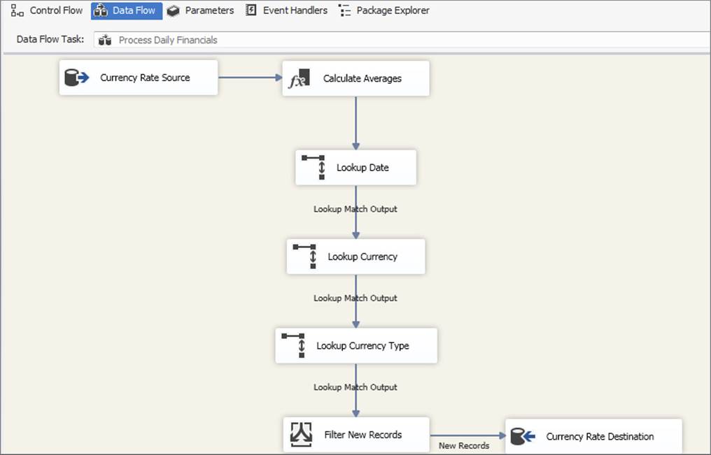
FIGURE 16-2
In other words, the first batch of data flowing in from the source may be in the final destination step (Currency Rate Destination), while at the same time data is still flowing in from the source.
Multiple components are running at the same time because the Data Flow Transformations are working together in a coordinated streaming fashion, and the data is being transformed in groups (called buffers) as it is passed down from the source to the subsequent transformations.
SSIS Package Execution Time from Package Start to Package Finish
Because a Data Flow is merely a type of Control Flow Task, and more than one Data Flow can be embedded in a package (or none!), the total time it takes to execute a package is measured from the execution of the first Control Flow Task or Tasks through the completion of the last task being executed, regardless of whether the components executing are Data Flow Transformations or Control Flow Tasks. This may sound obvious, but it is worth mentioning because when you are designing a package, maximizing the parallel processing where appropriate (with due regard to your server resources) helps optimize the flow and reduce the overall processing time.
The package shown in Figure 16-3 has several tasks executing a variety of processes and using precedence constraints in a way that demonstrates parallel execution of tasks. The last task, Back Up Database, is the only task that does not execute in parallel because it has to wait for the execution of all the other tasks. Because the Control Flow has been designed with parallelization, the overlap in tasks enables faster package execution than it would if the steps were executed in a serial manner as earlier shown (refer to Figure 16-1).
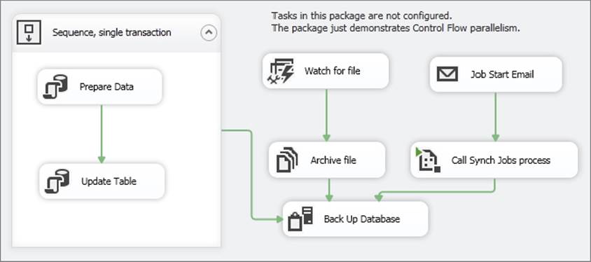
FIGURE 16-3
Handling Workflows with the Control Flow
Both of the components of the Control Flow have been discussed in Chapter 3, as well as the different types of precedence constraints. Because the Control Flow contains standard workflow concepts that are common to most scheduling and ETL tools, the rest of this chapter focuses on the Data Flow; however, a brief look at Control Flow parallelization and processing is warranted.
The Control Flow, as already mentioned, can be designed to execute tasks in parallel or serially, or a combination of the two. Tasks are also synchronous in nature, meaning a task requires completion before handing off an operation to another process. While it is possible to design a Control Flow containing tasks that are not connected with constraints to other tasks, the tasks are still synchronously tied to the execution of the package. Said in another way, a package cannot kick off the execution of a task and then complete execution while the task is still executing. Rather, the SSIS execution thread for the task is synchronously tied to the task’s execution and will not release until the task completes successfully or fails.
NOTE The synchronous nature of tasks should not be confused with the synchronous and asynchronous nature of transformations in the Data Flow. The concepts are slightly different. In the Data Flow, a transformation’s synchronicity is a matter of communication (how data is passed between transformations), rather than the process orientation of the Control Flow.
Data Processing in the Data Flow
The Data Flow is the core data processing factory of SSIS packages, where the primary data is handled, managed, transformed, integrated, and cleansed. Think of the Data Flow as a pipeline for data. A house, for example, has a primary water source, which is branched to all the different outlets in the house.
When a faucet is turned on, water flows out of it, while at the same time water is coming in from the source. If all the water outlets in a house are turned off, then the pressure backs up to the source to the point where water will no longer flow into the house until the pressure is relieved. Conversely, if all the water outlets in the house are opened at once, then the source pressure may not be able to keep up with the flow of water, and the pressure coming out of the faucets will be weaker. (Of course, don’t try this at home; it may produce other problems!)
The Data Flow is appropriately named because the data equates to the water in the plumbing analogy. The data flows from the Data Sources through the transformations to the Data Destinations. In addition to the flowing concept, there are similarities to the Data Flow pressure within the pipeline. For example, while a Data Source may be able to stream 10,000 rows per second, if a downstream transformation consumes too much server resources, it could apply backward pressure on the source and reduce the number of rows coming from the source. Essentially, this creates a bottleneck that may need to be addressed to optimize the flow. In order to understand and apply design principles in a Data Flow, an in-depth discussion of the Data Flow architecture is merited. Understanding several Data Flow concepts will give you a fuller perspective regarding what is going on under the hood of an executing package. Each of these concepts is addressed over the next few pages:
· Data buffer architecture
· Transformation types
· Transformation communication
· Execution trees
After reviewing the architecture, you can shift to monitoring packages in order to determine how the Data Flow engine handles data processing.
Memory Buffer Architecture
The Data Flow manages data in groups of data called buffers. A buffer is merely memory that is allocated for the use of storing rows and columns of data where transformations are applied. This means that as data is being extracted from sources into the engine, it is put into these preallocated memory buffers. Buffers are dynamically sized based on row width (the cumulative number of bytes in a row) and other package and server criteria. A buffer, for example, may include 9,000 rows of data with a few columns of data. Figure 16-4 shows a few groupings of buffers.
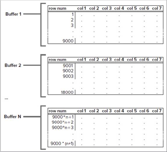
FIGURE 16-4
Although it is easy to imagine data being passed down from transformation to transformation in the Data Flow, like the flow of water in the pipeline analogy, this is not a complete picture of what is going on behind the scenes. Instead of data being passed down through the transformations, groups of transformations pass over the buffers of data and make in-place changes as defined by the transformations. Think of how much more efficient this process is than copying the data from one transformation to the next every time a transformation specified a change in the data! To be sure, there are times when the buffers are copied and other times when the buffers are held up in cache by transformations. Understanding how and when this happens will enable you to determine the best design to optimize your Data Flow.
This understanding of how memory buffers are managed requires knowing something about the different types of Data Flow Components — transformations, sources, and destinations.
Types of Transformations
The transformations in the Data Flow have certain characteristics that group each into different categories. The base-level differences between them are the way they communicate with each other, and how and when data is handed off from one transformation to another. Evaluating transformations on two fronts provides the background you need to understand how the buffers are managed:
· Blocking nature: Non-blocking (sometimes called streaming), semi-blocking, blocking
· Communication mechanism: Synchronous and asynchronous
In reality, these classifications are related, but from a practical standpoint, discussing them separately provides some context for data management in the Data Flow.
Non-Blocking, Semi-Blocking, and Blocking Transformations
The most obvious distinction between transformations is their blocking nature. All transformations fall into one of three categories: non-blocking, semi-blocking, or blocking. These terms describe whether data in a transformation is passed downstream in the pipeline immediately, in increments, or after all the data is fully received.
The blocking nature of a transformation is related to what a transformation is designed to accomplish. Because the Data Flow engine just invokes the transformations without knowing what they internally do, there are no properties of the transformation that discretely identify this nature. However, when we look at the communication between transformations in the next section (the synchronous and asynchronous communication), we can identify how the engine will manage transformations one to another.
Non-Blocking, Streaming, and Row-Based Transformations
Most of the SSIS transformations are non-blocking. This means that the transformation logic applied in the transformation does not impede the data from moving on to the next transformation after the transformation logic is applied to the row. Two categories of non-blocking transformations exist: streaming and row-based. The difference is whether the SSIS transformation can use internal information and processes to handle its work or whether the transformation has to call an external process to retrieve information it needs for the work. Some transformations can be categorized as streaming or row-based depending on their configuration, which are indicated in the list below.
Streaming transformations are usually able to apply transformation logic quickly, using precached data and processing calculations within the row being worked on. In these transformations, it is usually the case that a transformation will not slip behind the rate of the data being fed to it. These transformations focus their resources on the CPUs, which in most cases are not the bottleneck of an ETL system. Therefore, they are classified as streaming. The following transformations stream the data from transformation to transformation in the Data Flow:
· Audit
· Cache Transform
· Character Map
· Conditional Split
· Copy Column
· Data Conversion
· Derived Column
· Lookup (with a full-cache setting)
· Multicast
· Percent Sampling
· Row Count
· Script Component (provided the script is not configured with an asynchronous output, which is discussed in the “Advanced Data Flow Execution Concepts” section)
· Union All (the Union All acts like a streaming transformation but is actually a semi-blocking transformation because it communicates asynchronously, which is covered in the next section)
The second grouping of non-blocking transformations is identified as row-based. These transformations are still non-blocking in the sense that the data can flow immediately to the next transformation after the transformation logic is applied to the buffer. The row-based description indicates that the rows flowing through the transformation are acted on one by one with a requirement to interact with an outside process such as a database, file, or component. Given their row-based processes, in most cases these transformations may not be able to keep up with the rate at which the data is fed to them, and the buffers are held up until each row is processed. The following transformations are classified as row-based:
· DQS Cleansing
· Export Column
· Import Column
· Lookup (with a no-cache or partial-cache setting)
· OLE DB Command
· Script Component (where the script interacts with an external component)
· Slowly Changing Dimension (each row is looked up against the dimension in the database)
Figure 16-5 shows a Data Flow composed of only streaming transformations. If you look at the row counts in the design UI, you will notice that the transformations are passing rows downstream in the pipeline as soon as the transformation logic is completed. Streaming transformations do not have to wait for other operations in order for the rows being processed to be passed downstream.
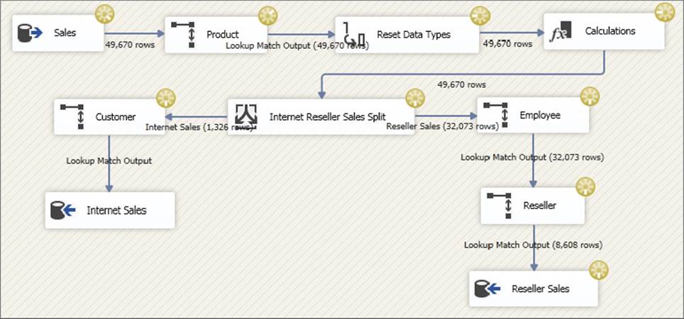
FIGURE 16-5
Also, notice in Figure 16-5 that data is inserted into the destination even while transformation logic is still being applied to some of the earlier transformations. This very simple Data Flow is handling a high volume of data with minimal resources, such as memory usage, because of the streaming nature of the Transformation Components used.
Semi-Blocking Transformations
The next category of Transformation Components are the ones that hold up records in the Data Flow for a period of time before allowing the memory buffers to be passed downstream. These are typically called semi-blocking transformations, given their nature. Only a few out-of-the-box transformations are semi-blocking in nature:
· Data Mining Query
· Merge
· Merge Join
· Pivot
· Term Lookup
· Unpivot
· Union All (also included in the streaming transformations list, but under the covers, the Union All is semi-blocking)
The Merge and Merge Join Transformations are described in detail in Chapter 4 and Chapter 7, but in relation to the semi-blocking nature of these components, note that they require the sources to be sorted on the matching keys of the merge. Both of these transformations function by waiting for key matches from both sides of the merge (or join), and when the matching sorted keys from both sides pass through the transformations, the records can then be sent downstream while the next set of keys is handled. Figure 16-6 shows how a Merge Join within a Data Flow will partially hold up the processing of the rows until the matches are made.
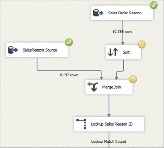
FIGURE 16-6
Typically, the row count upstream of the Merge Join is much higher than the row count just below the Merge Join, because the Merge Join waits for the sorted key matches as they flow in from both sides of the merge. Buffers are being released downstream, just not in a streaming fashion as in the non-blocking Transformation Components. You may also be wondering why there is no Sort Transformation on the right-side source of the Merge Join despite the fact that the transformations require the sources to be sorted. This is because the source data was presorted, and the Source component was configured to recognize that data flowing into the Data Flow was already sorted. Chapter 7 describes how to set the IsSorted property of a source.
NOTE Semi-blocking transformations require a little more server resources than non-blocking transformations because the buffers need to stay in memory until the right data is received.
In a large data processing situation, the question is how the Merge Join will handle a large data set coming in from one side of the join while waiting for the other set or if one source is slow and the other fast. The risk is exceeding the buffer memory while waiting. However, SSIS 2014 can throttle the sources by limiting the requests from the upstream transformations and sources, thereby preventing SSIS from getting into an out-of-memory situation. This very valuable engine feature of SSIS 2014 resolves the memory tension, enabling a Data Flow to continue without introducing a lot of data paging to disk in the process.
Blocking Transformations
The final category of transformation types is the actual blocking transformation. These components require a complete review of the upstream data before releasing any row downstream to the connected transformations and destinations. The list is also smaller than the list of non-blocking transformations because there are only a few transformations that require “blocking” all the data to complete an operation. Here is the list of the blocking transformations:
· Aggregate
· Fuzzy Grouping
· Fuzzy Lookup
· Row Sampling
· Sort
· Term Extraction
· Script Component (when configured to receive all rows before sending any downstream)
The two most widely used examples of the blocking transformations are the Sort and the Aggregate; each of these requires the entire data set before handing off the data to the next transformation. For example, in order to have an accurate average, all the records need to be held up by the Aggregate Transformation. Similarly, to sort data in a flow, all the data needs to be available to the Sort Transformation before the component knows the order in which to release records downstream. Figure 16-7 shows a Data Flow that contains an Aggregate Transformation. The screen capture of this process shows that the entire source has already been brought into the Data Flow, but no rows have been released downstream while the transformation is determining the order.
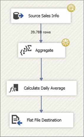
FIGURE 16-7
With a Blocking Component in the Data Flow (refer to Figure 16-7), the data is no longer streaming through the Data Flow. Instead, data is held up so that all the rows remain in the blocking transformation until the last row flows through the transformation.
NOTE Blocking transformations are usually more resource intensive than other types of transformations for two main reasons. First, because all the data is being held up, either the server must use a lot of memory to store the data or, if the server does not have enough memory, a process of file staging happens, which requires the I/O overhead of staging the data to disk temporarily. Second, these transformations usually put a heavy burden on the processor to perform the work of data aggregation, sorting, or fuzzy matching.
Synchronous and Asynchronous Transformation Outputs
Another important differentiation between transformations is related to how transformations that are connected to one another by a path communicate. While closely related to the discussion on the blocking nature of transformations, synchronous andasynchronous refer more to the relationship between the Input and Output Component connections and buffers.
Some transformations have an Advanced Editor window, which, among other things, drills into specific column-level properties of the transformations’ input and output columns, which is useful in understanding the difference between synchronous and asynchronous outputs. Figure 16-8 shows the Advanced Editor of the Sort Transformation, highlighting the Input and Output Properties tab. This particular transformation has a Sort Input and Sort Output group with a set of columns associated with each.
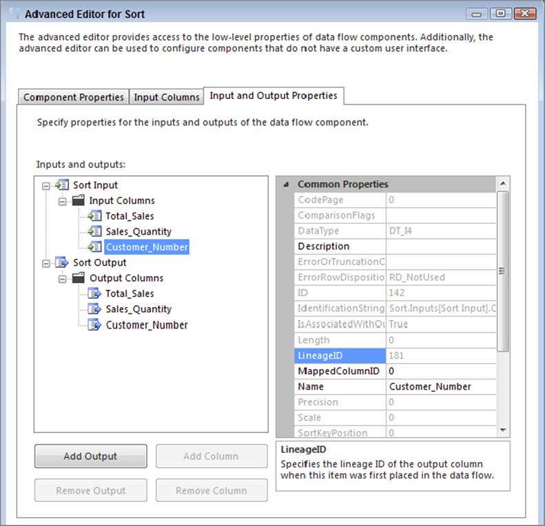
FIGURE 16-8
When a column is highlighted, the advanced properties of that column are displayed on the right, as shown in the figure. The advanced properties include such things as the data type of the column, the description, and so on. One important property to note is theLineageID. This is the integer pointer to the column within the buffers. Every column used in the Data Flow has at least one LineageID in the Data Flow. A column can have more than one LineageID as it passes through the Data Flow based on the types of transformation outputs (synchronous or asynchronous) that a column goes through in the Data Flow.
Asynchronous Transformation Outputs
It is easier to begin with the asynchronous definition because it leads into a comparison of the two kinds of transformation outputs, synchronous and asynchronous. A transformation output is asynchronous if the buffers used in the input are different from the buffers used in the output. In other words, many of the transformations cannot both perform the specified operation and preserve the buffers (the number of rows or the order of the rows), so a copy of the data must be made to accomplish the desired effect.
The Aggregate Transformation, for example, may output only a fraction of the number of rows coming into it; or when the Merge Join Transformation has to join two data sets together, the resulting number of rows may not be equivalent to the number of input rows. In both cases, the buffers are received, the processing is handled, and new buffers are created.
For example, returning to the Advanced Editor of the Sort dialog shown in Figure 16-8, note the LineageID property of the input column. In this transformation, all the input columns are duplicated in the output columns list. In fact, as Figure 16-9 shows, the output column highlighted for the same input has a different LineageID.
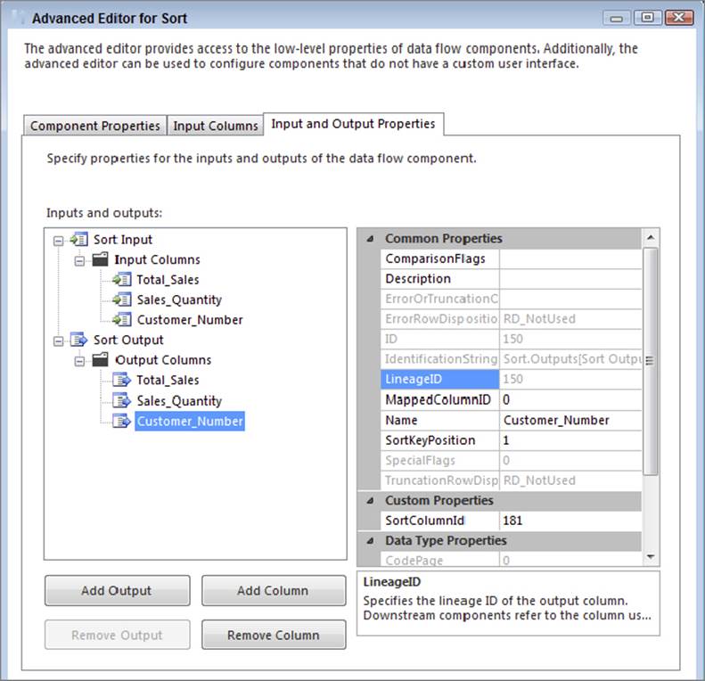
FIGURE 16-9
The LineageIDs are different for the same column because the Sort Transformation output is asynchronous, and the data buffers in the input are not the same buffers in the output; therefore, a new column identifier is needed for the output. In the preceding example, the input LineageID is 181, whereas in the output column the LineageID is 150.
A list doesn’t need to be included here, because all the semi-blocking and blocking transformations already listed have asynchronous outputs by definition — none of them can pass input buffers on downstream because the data is held up for processing and reorganized.
NOTE One of the SSIS engine components is called the buffer manager. For asynchronous component outputs, the buffer manager is busy at work, decommissioning buffers for use elsewhere (in sources or other asynchronous outputs) and reassigning new buffers to the data coming out of the transformation. The buffer manager also schedules processor threads to components as threads are needed.
Synchronous Transformation Outputs
A synchronous transformation is one in which the buffers are immediately handed off to the next downstream transformation at the completion of the transformation logic. If this sounds like the definition for streaming transformations, that’s because there is almost complete overlap between streaming transformations and synchronous transformations. The word buffers was intentionally used in the definition of synchronous outputs, because the important point is that the same buffers received by the transformation input are passed out the output.
The LineageIDs of the columns remain the same as the data is passed through the synchronous output, without a need to copy the buffer data and assign a new LineageID (as discussed previously for asynchronous transformation output).
To illustrate this point, refer back to Figure 16-5. In this example, each transformation, including the Conditional Split, has asynchronous outputs. This means that there are no buffer copies while this Data Flow runs. For the Source component called Sales, several of the columns are used in both the destinations. Now consider Figure 16-10, which shows the Advanced Editor of the source and highlights the TaxAmt column, which has a LineageID of 318.
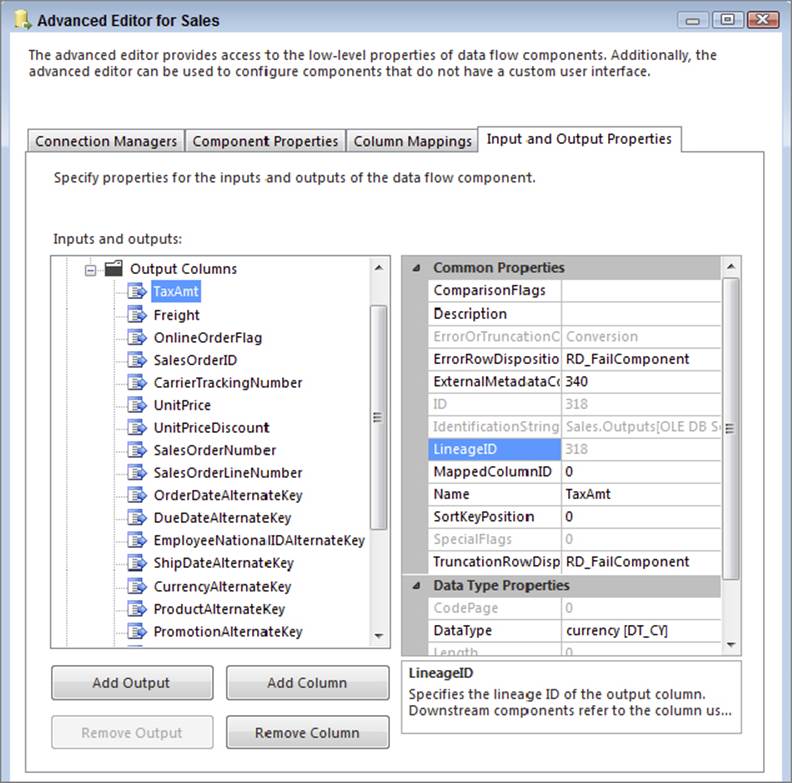
FIGURE 16-10
This LineageID for TaxAmt (as well as the other columns) is preserved throughout the Data Flow all the way to the destination. Figure 16-11 shows the Advanced Editor for one of the destination components, Reseller Sales, and indicates that the LineageID of 318 has been preserved through the entire Data Flow.
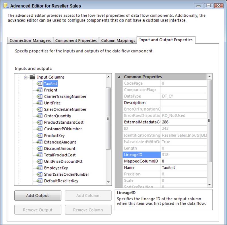
FIGURE 16-11
In fact, if you look at the LineageID of TaxAmt in the Internet Sales destination, you would also find that it is 299. Even for the Conditional Split (because it has asynchronous outputs), the data is not copied to new buffers; rather, the Data Flow engine maintains pointers to the right rows in the buffers, so if there is more than one destination, the data can be inserted into each destination without requiring data to be copied. This explains why the execution of the Data Flow shown earlier in Figure 16-5 allows the data to flow in a streaming way through the Data Flow.
NOTE A transformation is not limited to a single synchronous output. Both the Multicast and the Conditional Split can have multiple outputs, but all the outputs are synchronous.
With the exception of the Union All, all the non-blocking transformations listed in the previous section also have synchronous outputs. The Union All, while it functions like a streaming transformation, is really an asynchronous transformation. Given the complexity of unioning multiple sources together and keeping track of all the pointers to the right data from the different source inputs, the Union All instead copies the upstream data to new buffers as it receives them and passes the new buffers off to the downstream transformations.
NOTE Synchronous transformation outputs preserve the sort order of incoming data, whereas some of the asynchronous transformations do not. The Sort, Merge, and Merge Join asynchronous components, of course, have sorted outputs because of their nature, but the Union All, for example, does not.
A definitive way to identify synchronous versus asynchronous components is to look at the SynchronousInputID property of the Column Output properties. If this value is 0, the component output is asynchronous, but if this property is set to a value greater than 0, the transformation output is synchronous to the input whose ID matches the SynchronousInputID value.
Source and Destination Components
Source and Destination components are integral to the Data Flow and therefore merit brief consideration in this chapter. In fact, because of their differences in functionality, sources and destinations are therefore classified differently.
First of all, in looking at the advanced properties of a Source component, the source will have the same list of external columns and output columns. The external columns come directly from the source and are copied into the Data Flow buffers and subsequently assigned LineageIDs. While the external source columns do not have LineageIDs, the process is effectively the same as an asynchronous component output. Source components require the allocation of buffers, where the incoming data can be grouped and managed for the downstream transformations to perform work against.
Destination components, conversely, de-allocate the buffer data when it is loaded into the destinations. The advanced properties of the Destination component include an External Column list, which represents the destination columns used in the load. The input columns are mapped to this External Column list on the Mapping page of the Destination component editor. In the advanced properties, you should note that there is no primary Output Container (besides the Error Output) for the Destination component, as the buffers do not flow through the component but rather are committed to a Destination component as a final step in the Data Flow.
Advanced Data Flow Execution Concepts
The preceding discussion of transformation types and how outputs handle buffers leads into a more advanced discussion of how SSIS coordinates and manages Data Flow processing overall. This section ties together the discussion of synchronous and asynchronous transformations to provide the bigger picture of a package’s execution.
Relevant to this discussion is a more detailed understanding of buffer management within an executing package based on how the package is designed.
Execution Trees
In one sense, you have already looked at execution trees, although they weren’t explicitly referred to by this name. An execution tree is a logical grouping of Data Flow Components (transformations, sources, and destinations) based on their synchronous relationship to one another. Groupings are delineated by asynchronous component outputs that indicate the completion of one execution tree and the start of the next.
Figure 16-12 shows the execution trees of a moderately complex Data Flow that uses multiple components with asynchronous outputs. The “paths” indicated are numbered based on the SSIS Data Flow logging, not the order in which the data flows. See the PipelineExecutionTrees log example in the “Monitoring Data Flow Execution” section of this chapter.
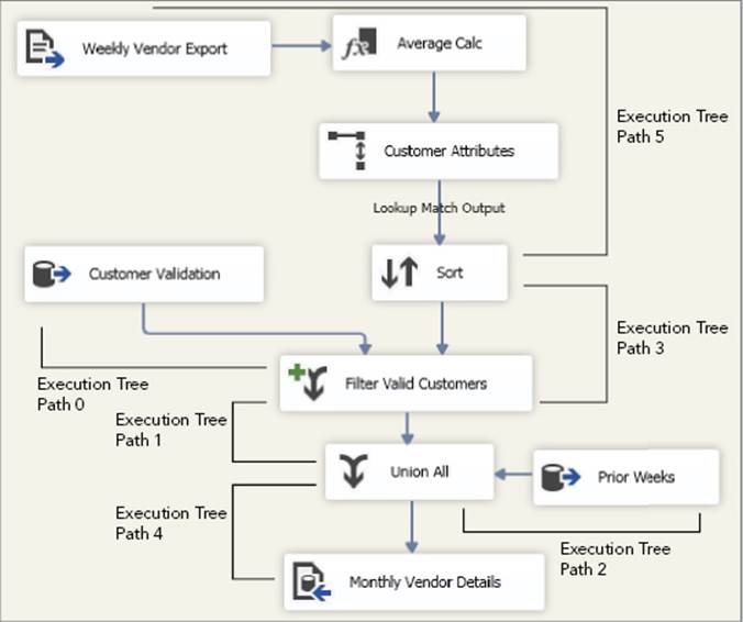
FIGURE 16-12
Recall that components with asynchronous outputs use different input buffers. The input participates in the upstream execution tree, while the asynchronous output begins the next execution tree. In light of this, the execution trees for Figure 16-12 start at the Source components and are then completed, and a new execution tree begins at every asynchronous transformation.
Execution trees are base 0, meaning you count them starting with a 0. In the next section, you will see how the pipeline logging identifies them. Although the execution trees seem out of order, you have used the explicit order given by the pipeline logging.
In the next section, you will look at ways to log and track the execution trees within a Data Flow, but for now the discussion focuses on a few principles that clarify what happens in an execution tree.
When SSIS executes a package, the buffer manager defines different buffer profiles based on the execution trees within a package. All the buffers used for a particular execution tree are identical in definition. When defining the buffer profile for each execution tree, the SSIS buffer manager looks at all the transformations used in the execution tree and includes every column in the buffer that is needed at any point within the execution tree. Note that execution tree path #5 in Figure 16-12 contains a Source component, a Derived Column Transformation, and a Lookup. Without looking at the source properties, the following list defines the four columns that the Source component is using from the source:
· CurrencyCode
· CurrencyRate
· AverageRate
· EndofDayRate
The Derived Column Transformation adds two more columns to the Data Flow: Average_Sale and Audit_Date. Finally, the Lookup Transformation adds another three columns to the Data Flow.
Added together, the columns used in these three components total nine. This means that the buffers used in this execution tree will have nine columns allocated, even though some of the columns are not used in the initial components. Optimizing a Data Flow can be compared to optimizing a relational table, where the smaller the width and number of columns, the more that can fit into a Data Flow buffer. This has some performance implications, and the next section looks in more detail at optimizing buffers.
When a buffer is used in an execution tree and reaches the transformation input of the asynchronous component (the last step in the execution tree), the data is subsequently not needed because it has been passed off to a new execution tree and a new set of buffers. At this point, the buffer manager can use the allocated buffer for other purposes in the Data Flow.
NOTE One final note about execution trees — the process thread scheduler can assign more than one thread to a single execution tree if threads are available and the execution tree requires intense processor utilization. Each transformation can receive a single thread, so if an execution tree has only two components that participate, then the execution tree can have a maximum of two threads. In addition, each source component receives a separate thread.
One advanced property of the Data Flow is the EngineThreads property. In the Control Flow, when a Data Flow Task is highlighted, this property appears in the Properties window list (see Figure 16-13).
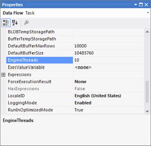
FIGURE 16-13
It is important to modify the EngineThreads property of the Data Flow so that the execution trees are not sharing process threads, and extra threads are available for large or complex execution trees. Furthermore, all the execution trees in a package share the number of processor threads allocated in the EngineThreads property of the Data Flow. A single thread or multiple threads are assigned to an execution tree based on availability of threads and complexity of the execution tree.
In the last section of this chapter, you will see how the threads available in a Data Flow are allocated to the execution trees. The value for EngineThreads does not include the threads allocated for the number of sources in a Data Flow, which are automatically allocated separate threads.
Monitoring Data Flow Execution
Built into SSIS 2014 is the capability to report on Data Flow performance and identify execution trees and threads. The reports and log events can be very useful in understanding your Data Flow and how the engine is managing buffers and execution.
First of all, pipeline logging events are available in the Logging features of SSIS. As shown in the following list, several logging events provide details about what is happening in the Data Flow. Books Online describes each of these in detail, with examples, athttp://msdn.microsoft.com/en-us/library/ms141122(v=SQL.120).aspx.
· OnPipelinePostEndOfRowset
· OnPipelinePostPrimeOutput
· OnPipelinePreEndOfRowset
· OnPipelinePrePrimeOutput
· OnPipelineRowsSent
· PipelineBufferLeak
· PipelineComponentTime
· PipelineExecutionPlan
· PipelineExecutionTrees
· PipelineInitialization
NOTE When executing a package on the SSIS server, you can turn on the Verbose logging to capture all the events. This is found on the Advanced tab of the Execute Package dialog under Logging level.
To better understand execution trees, you can capture the PipelineExecutionTrees log event. To do so, create a new log entry through the logging designer window under the SSIS menu’s Logging option. The pipeline events are available only when a Data Flow is selected in the tree menu navigator of the package executable navigator, as shown in Figure 16-14.
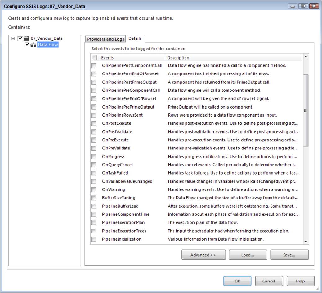
FIGURE 16-14
On the Details tab of this Configure SSIS Logs dialog, the two execution information log events just listed are available to capture. When the package is run, these events can be tracked to the selected log provider as defined. However, during development, it is useful to see these events when testing and designing a package. SSIS includes a way to see these events in the SQL Server Data Tools as a separate window. The Log Events window can be pulled up either from the SSIS menu by selecting Log Events or through the View menu, listed under the Other Windows submenu.
When the package is executed in design time through the interface, the log events selected are displayed in the Log Events window. For each Data Flow, there is one event returned for the PipelineExecutionPlan event and one for the PipelineExecutionTrees event, as shown in Figure 16-15. These log details have been captured from the sample Data Flow used in Figure 16-12.
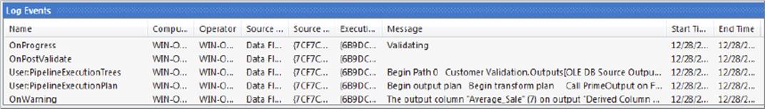
FIGURE 16-15
Note that all pipeline events selected in the Logging configuration are included in the Log window. To capture the details for a more readable view of the Message column, simply right-click the log entry and copy, which puts the event message onto the clipboard.
Pipeline Execution Trees Log Details
The PipelineExecutionTrees log event describes the grouping of transformation inputs and outputs that participate in each execution tree. Each execution tree is numbered for readability. The following text comes from the message column of the PipelineExecutionTrees log entry from the execution of the Data Flow shown in Figure 16-12:
Begin Path 0
Customer Validation.Outputs[OLE DB Source Output]; Customer Validation
Filter Valid Customers.Inputs[Merge Join Right Input]; Filter Valid Customers
End Path 0
Begin Path 1
Filter Valid Customers.Outputs[Merge Join Output]; Filter Valid Customers
Union All.Inputs[Union All Input 1]; Union All
End Path 1
Begin Path 2
Prior Weeks.Outputs[OLE DB Source Output]; Prior Weeks
Union All.Inputs[Union All Input 2]; Union All
End Path 2
Begin Path 3
Sort.Outputs[Sort Output]; Sort
Filter Valid Customers.Inputs[Merge Join Left Input]; Filter Valid Customers
End Path 3
Begin Path 4
Union All.Outputs[Union All Output 1]; Union All
Monthly Vendor Details.Inputs[SQL Server Destination Input]; Monthly Vendor
Details
End Path 4
Begin Path 5
Weekly Vendor Export.Outputs[Flat File Source Output]; Weekly Vendor Export
Average Calc.Inputs[Derived Column Input]; Average Calc
Average Calc.Outputs[Derived Column Output]; Average Calc
Customer Attributes.Inputs[Lookup Input]; Customer Attributes
Customer Attributes.Outputs[Lookup Match Output]; Customer Attributes
Sort.Inputs[Sort Input]; Sort
End Path 5
In the log output, each execution tree evaluated by the engine is listed with a begin path and an end path, with the transformation inputs and outputs that participate in the execution tree. Some execution trees may have several synchronous component outputs participating in the grouping, while others may be composed of only an input and output between two asynchronous components. As mentioned earlier, the execution trees use base 0, so the total number of execution trees for your Data Flow will be the numeral of the last execution tree plus one. In this example, there are six execution trees. A quick way to identify synchronous and asynchronous transformation outputs in your Data Flow is to review this log. Any transformation for which both the inputs and the outputs are contained within one execution tree is synchronous. Conversely, any transformation for which one or more inputs are separated from the outputs in different execution trees has asynchronous outputs.
Pipeline Execution Reporting
SSIS 2014 comes with a set of execution and status reports that highlight the current executions, history, and errors of package execution. Chapter 22 covers the reports in general. These reports are available only if you have your packages in the project deployment model, have deployed them to an SSIS server, and run the package on the server. In addition to the report highlighted later, you can also query the execution data in the SSISDB database on the server. The log information named in SSIS 2014 is available in the catalog. In addition, there is a table-value function catalog.dm_execution_performance_counters that can provide execution instance-specific information such as the number of buffers used.
One very valuable data collection point for Data Flow execution is the “Active Time” (in seconds) of each Data Flow Component. If you want to know how long a transformation is being used during a Data Flow execution, you can compare the active time to the total time of the Data Flow. In order to capture these details, you need to enable the performance logging level when the package is executed. Figure 16-16 shows the Advanced tab of the Execute Package window when executing a package on the SSIS server.
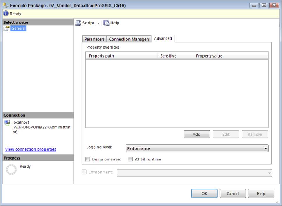
FIGURE 16-16
This logging level is also available in SQL Server Agent when you schedule a package to be run through the SQL Server Integration Services Package job step.
The benefit of logging this level of detail for a package is that it retains the performance details of the Data Flow. If you run the Execution Performance report (right-click the package in the SSIS Catalog project and run the All Executions report, then drill down to Execution Performance), you can see the history of the package, as well as the Data Flow Components and how long each were active. Figure 16-17 shows a sample Execution Performance report.
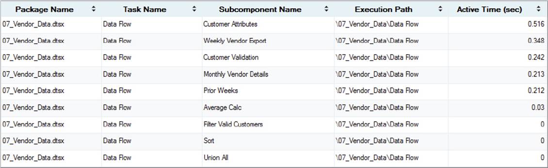
FIGURE 16-17
As you can imagine, if you are having performance problems with your Data Flows, you can run this report and quickly identify the trouble spots that you need to work on. The next section describes ways to efficiently design, optimize, and tune your Data Flow.
SSIS DATA FLOW DESIGN AND TUNING
Now that you know how the Data Flow engine works, it will be easier to understand Data Flow design principles and tuning practices.
Designing a data-processing solution requires more than just sending the source data into a black-box transformation engine with outputs that push the data into the destination. Of course, system requirements will dictate the final design of the process, including but not limited to the following:
· Source and destination system impact
· Processing time windows and performance
· Destination system state consistency
· Hard and soft exception handling and restartability needs
· Environment architecture model, distributed hardware, or scaled-up servers
· Solution architecture requirements, such as flexibility of change or OEM targeted solutions
· Modular and configurable solution needs
· Manageability and administration requirements
Looking at this list, you can quickly map several of these items to what you have learned about SSIS already. In most cases, a good architecture leverages the built-in functionality of the tool, which reduces administrative and support requirements. The tool selection process, if it is not completed before a solution is developed, should include a consideration of the system requirements and the functionality of available products.
Data Flow Design Practices
Keep the following four design practices in mind when creating new packages:
· Limit synchronous processes
· Monitor the memory use of blocking and semi-blocking transformations
· Reduce staging and disk I/O
· Reduce reliance on an RDBMS
To limit synchronous processes, you should be conscious of processes that need to complete before the next process begins. For example, if you run a long INSERT T-SQL statement that takes one-half hour to complete, and then run an UPDATE statement that updates the same table, the UPDATE statement cannot run until the INSERT script finishes. These processes are synchronous. In this case, it would be better to design a Data Flow that handles the same logic as the INSERT statement and combines the UPDATE logic at the same time (also using a SQL UPDATE); that way, you are not only taking advantage of the Data Flow but making the logic asynchronous. You can seriously reduce overall process times by taking this approach.
As mentioned earlier, blocking and semi-blocking transformations require buffers to be pooled in memory until either the last row is available or a match is received (in the case of a Merge Join). These transformations can be very useful, but you need to ensure that you have sufficient memory on your server in order for them to perform well. If you have a large aggregate operation across 100 million rows, you are likely better off handling this through the SQL Server relational engine.
Reducing disk I/O is about minimizing the staging requirements in your ETL process. Disk I/O is often the biggest bottleneck in an ETL job because the bulk operations involve moving a lot of data, and when you add staging data to a database, that data ultimately needs to be saved to the disk drives. Instead, reduce your need on staging tables and leverage the Data Flow for those same operations; that way, you decrease the disk overhead of the process and achieve better scalability. The Data Flow primarily uses memory, and memory is a lot faster to access than disks, so you will gain significant improvements in terms of speed. In addition, when you stage data to a table, you are doubling the disk I/O of the data, because you are both inserting and retrieving table data.
Keep in mind that solution requirements often drive design decisions, and there are situations where staging or the RDBMS are useful in data processing. Some of these are discussed in this section. Your goal, though, is to rethink your design paradigms with SSIS.
Reducing the RDBMS reliance is similar to reducing staging environments, but it also means reducing the logic you place on the DBMS to perform operations like grouping and data cleansing. This not only reduces the impact on your RDBMS, but when using production databases, it alleviates the load and makes room for more critical RDBMS operations.
These four principles are worked out further in the next section, which discusses ways to leverage the Data Flow for your ETL operations.
Leveraging the Data Flow
The biggest value that SSIS brings is the power of the Data Flow. Not to minimize the out-of-the-box functionality of restartability, configurations, logging, event handlers, or other Control Flow Tasks, the primary goal of the engine is to “integrate,” and the Data Flow is the key to realizing that goal. Accomplishing data-processing logic through Data Flow Transformations provides enhanced performance and greater flexibility.
Many data architects come from DBA backgrounds, so when they are trying to solve a data integration, processing, or cleansing scenario, their first impulse is to use an RDBMS, such as SQL Server, for ETL operations.
In some ways, moving to SSIS requires thinking in different terms — Data Flow terms. In previous chapters, you looked at the different Data Flow Transformations, so the focus in this section is on applying some of those components to design decisions and translating the SQL-based designs into Data Flow processes.
In summary, the four architecture best practices described in the preceding section relate directly to the value that the Data Flow provides:
· Limit synchronous processes: By bringing more of the processing logic into the Data Flow, the natural result is fewer process-oriented steps that require completion before proceeding. In the previous chapter, you looked at the general streaming nature of the Data Flow. This translates to reduced overall processing times.
· Monitor the memory use of blocking and semi-blocking transformations: When memory becomes scarce on your server, SSIS begins to copy buffers to disk or spool them to disk. Once this happens, your package slows down dramatically. The most intensive memory transformations are blocking and semi-blocking transformations. However, other transformations, like the cached Lookup, also can require a lot of memory if the Lookup table contains millions of items. All these transformations perform very well until they near the threshold of memory on your server. It is best to monitor the memory to ensure that you avoid a low-memory situation. In particular, throttle the memory of SQL Server if it is on the same server where your SSIS packages are running.
· Reduce staging and expensive IO operations: The Data Flow performs most operations in memory (with occasional use of temp folders and some interaction with external systems). Whenever processing happens on data that resides in RAM, processing is more efficient. Disk I/O operations rely on the performance of the drives, the throughput of the I/O channels, and the overhead of the operating system to write and read information to and from the disk. With high volumes or bursting scenarios typical with data processing and ETL, disk I/O is often a bottleneck.
· Reduce reliance on RDBMS: Relational engines are powerful tools, and the point here is not to detract from their appropriate uses to store and manage data. By using the Data Flow to cleanse and join data rather than the RDBMS, the result is reduced impact on the relational system, which frees it up for other functions that may be higher priority. Reading data from a database is generally less expensive than performing complex joins or complicated queries. In addition, related to the first bullet, all RDBMS operations are synchronous. Set-based operations, while they are very useful and optimized in a relational database system, still require that the operation be complete before the data is available for other purposes. The Data Flow, conversely, can process joins and Lookups and other cleansing steps in parallel while the data is flowing through the pipeline. However, note that an RDBMS engine can be leveraged in certain ways; for example, if a table has the right indexes, you can use an ORDER BY, which may be faster than an SSIS Sort Transformation.
Data Integration and Correlation
As discussed in Chapter 7, the Data Flow provides the means to combine data from different source objects completely independent of the connection source where the data originates. The most obvious benefit of this is the ability to perform in-memory correlation operations against heterogeneous data without having to stage the data. Said in another way, with SSIS, you can extract data from a flat file and join it to data from a database table inside the Data Flow, without first having to stage the flat file to a table and then perform a SQL Join operation. This can be valuable even when the data is coming from the same source, such as a relational database engine; source data extractions are more efficient without complex or expensive joins, and data can usually begin to flow into the Data Flow immediately.
In addition, single-table SELECT statements provide less impact on the source systems than do pulls where join logic is applied. Certainly there are situations where joining data in the source system may be useful and efficient; in many cases, however, focusing on data integration within the Data Flow will yield better performance. When different source systems are involved, the need to stage the data is reduced.
Several of the built-in transformations can perform data correlation similar to how a database would handle joins and other more complex data relationship logic. The following transformations provide data association for more than one Data Source:
· Lookup
· Merge Join
· Merge
· Union All
· Fuzzy Lookup
· Term Lookup
· Term Extract
Chapter 7 describes how to leverage the joining capabilities of SSIS, a great reference for designing your SSIS Data Flows.
Furthermore, beyond the built-in capabilities of SSIS, custom components allow more complex or unique scenarios to be handled. This is discussed in Chapter 19.
Data Cleansing and Transformation
The second major area to which you can apply the Data Flow is data cleansing. As discussed in Chapter 10, cleansing data involves managing missing values; correcting out-of-date, incomplete, or miskeyed data; converting values to standard data types; changing data grain or filtering data subsets; and de-duplicating redundant data. Consistency is the goal of data cleansing, whether the Data Source is a single system or multiple disparate sources.
Many of the Data Flow Components provide data-cleansing capabilities or can participate in a data-cleansing process. Some of the more explicit transformations usable for this process include the following:
· Aggregate
· Character Map
· Conditional Split
· Data Conversion
· Derived Column
· DQS Cleansing
· Fuzzy Grouping
· Fuzzy Lookup
· Pivot
· Script Component
· Sort (with de-duplicating capabilities)
· Unpivot
Each of these transformations, or a combination of them, can handle many data-cleansing scenarios. A few of the transformations provide compelling data-cleansing features that even go beyond the capabilities of many relational engines by using the Data Flow. For example, the Fuzzy Lookup and Fuzzy Grouping (de-duplication) provide cleansing of dirty data by comparing data similarity within certain defined ranges. Pivot and Unpivot have the ability to transform data coming in by pivoting rows to columns or vice versa.
Also, the Script Transformation offers very powerful data-cleansing capabilities with the full features of VB.NET embedded; it is highlighted in detail in Chapter 9. Because the goal of this chapter is to discuss the application of SSIS, the example focuses on a couple of common examples of data cleansing using the Derived Column Transformation and the Aggregate Transformation. These two transformations are particularly relevant to how data cleansing can be accomplished in the Data Flow in comparison with common query logic.
Staging Environments
So far in this chapter, the emphasis has been on thinking in Data Flow terms by moving core data process logic into the Data Flow. In most cases, this will yield high-performance results, especially when the timeliness of moving the data from point A to point B is the highest priority, such as in near real-time or tight-processing-window scenarios. Doing this also mitigates some management overhead, limiting interim database usage.
A few situations merit staging environments and are worth mentioning for consideration:
· Restartability: The built-in checkpoint logic of SSIS revolves around the Control Flow. This means that a failure in the Data Flow will not persist the data state. Rather, when the package is restarted, the Data Flow will restart from the beginning. The implications affect design if the source system is in flux and an error in the Data Flow causes a processing window to be missed. By landing the raw data first, the chance for data errors is minimized, and in the event of a failure during the load process, the package can be restarted from the staged data.
· Processing windows and precedence: Certain requirements may dictate that the various source extraction windows do not line up with each other or with the data load window for the destination. In these scenarios, it would be necessary to stage the data for a period of time until the full data set is available or the destination database load window has been reached.
· Source backpressure: At times, the Data Flow Transformations may apply backpressure on the source extractions. This would happen when the flow of incoming data is faster than the ability of the transformations to handle the data processing in the pipeline. The backpressure created slows down the extraction on the source system, and if the requirement is to extract the data in the fastest time with the least impact, then staging the raw data extract may help eliminate the backpressure.
· Data Flow optimization: Staging certain elements, such as business keys, can actually provide valuable data to optimize the primary Data Flow. For example, if the Lookup Source query can be filtered based on a set of keys that was prestaged, this may allow overall gains in processing times by reducing the time it takes to load the Lookup plus the amount of memory needed for the operation. A second example is the use of staging to perform set-based table updates. Updates in a large system are often the source of system bottlenecks, and because SSIS cannot perform set-based updates in the Data Flow, one solution is to stage tables that can be used in a later Execute SQL Task for a set-based update, which may provide a more efficient process.
Staged data can also prove useful in data validation and error handling. Given some of the uses of staging, is there a way to accomplish data staging but still retain the performance gain by leveraging the Data Flow? Yes. One suggestion is the reduction of synchronous processing in the Control Flow. When you want to introduce a data-staging environment, it’s natural to first pick up the data from the source and land it to a staging environment, and then pick the data back up from the staging environment and apply the transformation logic to it; but what about landing the raw data to a staging environment at the same time that the transformations are applied? Figure 16-18 shows a Data Flow designed with a staging table that does not require the data to reside in the table before the transformation logic is applied.
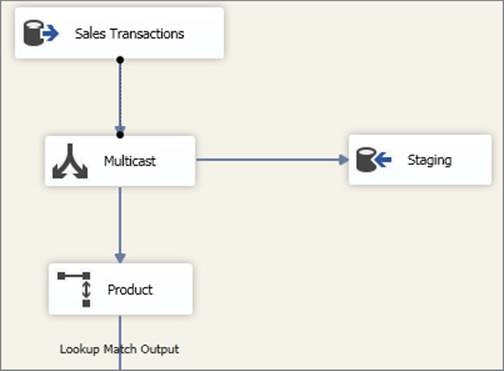
FIGURE 16-18
The Multicast Transformation in this example is taking the raw source data and allowing it to stream down to the core Data Flow, while at the same time the raw source data is being staged to a table. The data within the table is now available to query for data validation and checking purposes; in addition, it provides a snapshot of the source system that can then be used for reprocessing when needed. Although the data is landed to staging, two differences distinguish this example from a model that first stages data and then uses the staged data as a source.
First, as already mentioned, the process is no longer synchronous; in many cases, data can move from point A to point B in the time it takes to simply extract the data from A. Second, the staging process requires only a single pass on the staging table (for the writes), rather than the I/O overhead of a second pass that reads the data from the staging. If your restartability requirements and source systems allow, this approach may provide the best of both worlds — leveraging the Data Flow but providing the value of a staging environment.
Optimizing Package Processing
There are a few techniques you can apply when you’re streamlining packages for performance. This section covers how to apply certain optimization techniques to achieve better throughput.
Optimizing Buffers, Execution Trees, and Engine Threads
Recall from earlier in this chapter that for each execution tree in a Data Flow, a different buffer profile is used. This means that downstream execution trees may require different columns based on what is added or subtracted in the Data Flow. You also saw that the performance of a buffer within a Data Flow is directly related to the row width of the buffer. Narrow buffers can hold more rows, enabling higher throughput.
Some columns that are used in an execution tree may not be needed downstream. For example, if an input column to a Lookup Transformation is used as the key match to the reference table, this column may not be needed after the Lookup and therefore should be removed before the next execution tree. SSIS does a good job of providing warnings when columns exist in an execution tree but are not used in any downstream transformation or destination component. Figure 16-19 shows the Execution Results tab (also called the Progress tab when in runtime mode) within a package for which column usage has not been optimized in the Data Flow. Each warning, highlighted with a yellow exclamation point, indicates the existence of a column not used later in downstream components and which therefore should be removed from the pipeline after initial use.
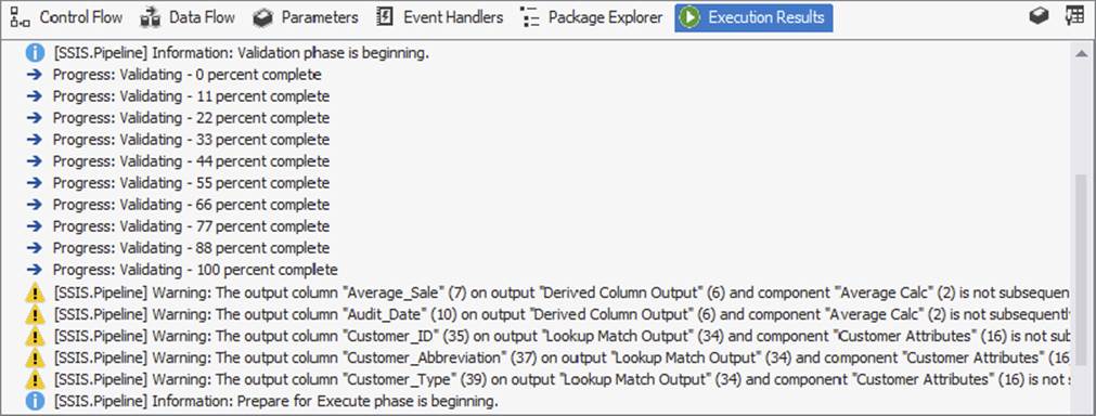
FIGURE 16-19
The warning text describes the optimization technique well:
[SSIS.Pipeline] Warning: The output column "Average_Sale" (7) on output "Derived
Column Output" (6) and component "Average Calc" (2) is not subsequently used in
the Data Flow task. Removing this unused output column can increase Data Flow task
performance.
Any component with asynchronous outputs whose input closes out an execution tree has the option of removing columns in the output. You would normally do this through the edit dialog of the transformation, but you can also do it in the Advanced Editor if the component provides an advanced properties window. For example, in the Union All Transformation, you can highlight a row in the editor and delete it with the Delete keyboard key. This ensures that the column is not used in the next execution tree.
A second optimization technique involves increasing processor utilization by adding the more execution threads for the Data Flow. Increasing the EngineThreads Data Flow property to a value greater than the number of execution trees plus the number of Source Components ensures that SSIS has enough threads to use.
Careful Use of Row-Based Transformations
Row-based transformations, as described earlier in this chapter, are non-blocking transformations, but they exhibit the functionality of interacting with an outside system (for example, a database or file system) on a row-by-row basis. Compared with other non-blocking transformations, these transformations are slower because of this behavior. The other type of non-blocking transformation, streaming, can use internal cache or provide calculations using other columns or variables readily available to the Data Flow, making them perform very fast. Given the nature of row-based transformations, their usage should be cautious and calculated.
Of course, some row-based transformations have critical functionality, so this caution needs to be balanced with data-processing requirements. For example, the Export and Import Column Transformation can read and write from files to columns, which is a very valuable tool, but it has the obvious overhead of the I/O activity with the file system.
Another useful row-based transformation is the OLE DB Command, which can use input column values and execute parameterized queries against a database, row by row. The interaction with the database, although it can be optimized, still requires overhead to process. Figure 16-20 shows a SQL Server Trace run against a database that is receiving updates from an OLE DB Command.
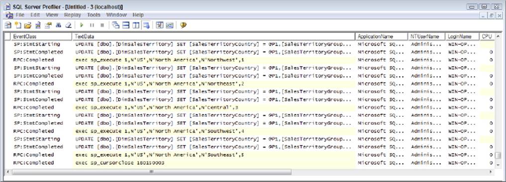
FIGURE 16-20
This is only a simple example, but for each row that goes through the OLE DB Command, a separate UPDATE statement is issued against the database. Taking into consideration the duration, reads, and writes, the aggregated impact of thousands of rows will cause Data Flow latency at the transformation.
For this scenario, one alternative is to leverage set-based processes within databases. In order to do this, the data needs to be staged during the Data Flow, and you need to add a secondary Execute SQL Task to the Control Flow that runs the set-based update statement. The result may actually reduce the overall processing time when compared with the original OLE DB Command approach. This alternative approach is not meant to diminish the usefulness of the OLE DB Command but rather meant to provide an example of optimizing the Data Flow for higher-volume scenarios that may require optimization.
Understanding Blocking Transformation Effects
A blocking transformation requires the complete set of records cached from the input before it can release records downstream. Earlier in the chapter, you saw a list of nearly a dozen transformations that meet this criterion. The most common examples are the Sort and Aggregate Transformations.
Blocking transformations are intensive because they require caching all the upstream input data, and they also may require more intensive processor usage based on their functionality. When not enough RAM is available in the system, the blocking transformations may also require temporary disk storage. You need to be aware of these limitations when you try to optimize a Data Flow. Mentioning the limitations of blocking transformations is not meant to minimize their usefulness. Rather it’s to emphasize how important it is to understand when to use these transformations as opposed to alternative approaches and to know the resource impact they may have.
Because sorting data is a common requirement, one optimization technique is valuable to mention. Source data that can be sorted in the component through an ORDER BY statement (if the right indexes are in the source table) or presorted in a flat file does not require the use of a Sort Transformation. As long as the data is physically sorted in the right order when entering the Data Flow, the Source component can be configured to indicate that the data is sorted and which columns are sorted in what order. As mentioned earlier, theIsSorted advanced property of the Source component is documented in Chapter 7.
Troubleshooting Data Flow Performance Bottlenecks
The pipeline execution reports (reviewed earlier in the chapter) are a great way to identify which component in your Data Flow is causing a bottleneck. Another way to troubleshoot Data Flow performance is to isolate transformations and sources by themselves.
While you are developing your package, you can identify bottlenecks within a specific Data Flow by making a copy of your Data Flow and begin decomposing it by replacing components with placeholder transformations. In other words, take a copy of your Data Flow and run it without any changes. This will give you a baseline of the execution time of the package.
Next, remove all the Destination components, and replace them with Multicast Transformations (the Multicast is a great placeholder transformation because it can act as a destination without any outputs and has no overhead). Figure 16-21 represents a modified package in which the Destination components have been replaced with Multicast Transformations.
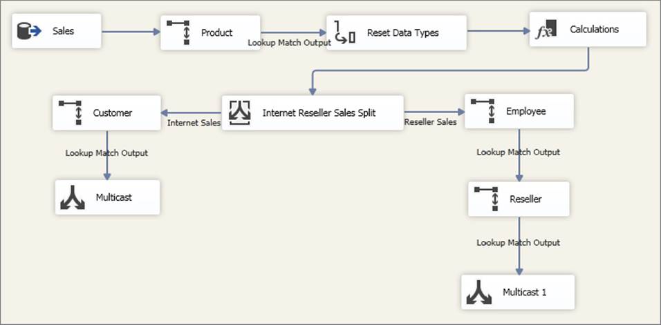
FIGURE 16-21
Run this modified Data Flow and evaluate your execution time. Is it a lot faster? If so, you have identified your problem — it’s one or more of your destinations.
If your package without the destinations still runs the same, then your performance bottleneck is a source or one of the transformations. The next most common issue is the source, so this time, delete all your transformations and replace them with Multicast Transformations, as Figure 16-22 shows.
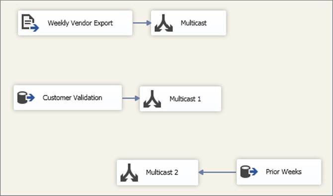
FIGURE 16-22
Run your package. If the execution time is just as slow as the first run, then you can be sure that the performance issue is one or more of the sources. If the performance is a lot faster, then you have a performance issue with one of the transformations. Even the Active Time report shown in Figure 16-17 can give deceptive results if the source is the bottleneck. The source and all transformations in the first execution tree will show high active time. In fact, all your Data Flow components may have a high active time if you don’t have any blocking transformations. Therefore, checking the sources will assist in identifying whether the Source component is the hidden bottleneck.
In fact, the Multicast approach can be applied repeatedly until you figure out where the issue lies. In other words, go back to your original copy of the Data Flow and replace transformations until you have identified the transformation that causes the biggest slowdown. It may be the case that you have more than one component that is the culprit, but with this approach you will know where to focus your redesign or reconfiguration efforts.
PIPELINE PERFORMANCE MONITORING
Earlier in this chapter, you looked at the built-in pipeline logging functionality and the active time reports and how they can help you understand what SSIS is doing behind the scenes when running a package with one or more Data Flows. Another tool available to SSIS is the Windows operating system tool called Performance Monitor (PerfMon for short), which is available to local administrators in the machine’s Administrative Tools. When SSIS is installed on a machine, a set of counters is added that enables tracking of the Data Flow’s performance.
As Figure 16-23 shows, the Pipeline counters can be used when selecting the SQLServer:SSIS Pipeline 12.0 object.
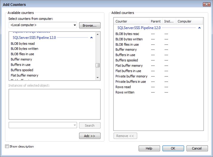
FIGURE 16-23
The following counters are available in the SQLServer:SSIS Pipeline object within PerfMon. Descriptions of these counters are provided next:
· BLOB bytes read
· BLOB bytes written
· BLOB files in use
· Buffer memory
· Buffers in use
· Buffers spooled
· Flat buffer memory
· Flat buffers in use
· Private buffer memory
· Private buffers in use
· Rows read
· Rows written
The BLOB counters (Binary Large Objects, such as images) help identify the volume of the BLOB data types flowing through the Data Flow. Because handling large binary columns can be a huge drain on the available memory, understanding how your Data Flow is handling BLOB data types is important. Remember that BLOB data can be introduced to the Data Flow not only by Source components but also by the Import (and Export) Column Transformations.
Because buffers are the mechanism that the Data Flow uses to process all data, the buffer-related counters provide the most valuable information for understanding how much and where memory is being used in the Data Flow. The Buffer Memory and Buffers in Use counters are high-level counters that provide totals for the server, both memory use and total buffer count. Essentially, the Buffer Memory counter shows the total memory being used by SSIS, and this can be compared with the amount of available system memory to determine whether SSIS processing is bottlenecked by the available physical memory. Furthermore, the Buffers Spooled counter provides even more indication of resource limitations on your server. It shows the number of buffers temporarily written to disk if enough system memory is not available. Anything greater than zero indicates that your Data Flow is using temporary disk storage to accomplish its work, which incurs I/O impact and overhead.
In regard to the buffer details, two types of buffers exist, flat and private. Flat buffers are the primary Data Flow buffers used when a Source component sends data into the Data Flow. Synchronous transformation outputs pass the flat buffers to the next component, and asynchronous outputs use reprovisioned or new flat buffers to be passed to the next transformation. Conversely, some transformations require private buffers, which are not received from upstream transformations or passed on to downstream transformations. Instead, they represent a private cache of data that a transformation uses to perform its operation. Three primary examples of private buffer use are found in the Aggregate, Sort, and Lookup Transformations, which use private buffers to cache data that is used for calculations and matching. These transformations still use flat buffers for data being received and passed, but they also use private buffers to manage and cache supplemental data used in the transformation. The flat and private buffer counters show the breakdown of these usages and help identify where buffers are being used and to what extent.
The last counters in the Pipeline counters list simply show the number of rows handled in the Data Flow, whether Rows Read or Rows Written. These numbers are aggregates of the rows processed since the counters were started.
When reviewing these counters, remember that they are an aggregate of all the SSIS packages and embedded Data Flows running on your server. If you are attempting to isolate the performance impact of specific Data Flows or packages, consider querying the catalog.dm_execution_performance_counters in the SSISDB database.
The Pipeline counters can be tracked in the UI of Performance Monitor in real time or captured at a recurring interval for later evaluation. Figure 16-24 shows the Pipeline counters tracked during the execution of a package.
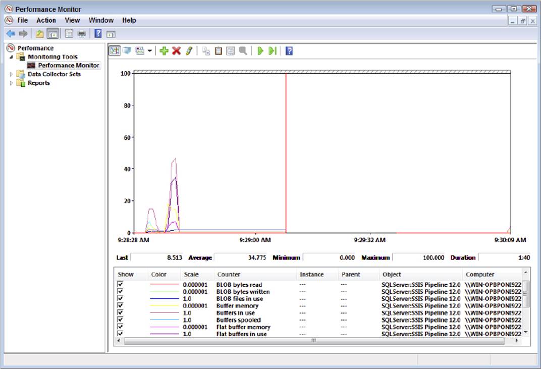
FIGURE 16-24
Notice that the buffer usage scales up and then drops and that the plateau lines occur during the database commit process, when SSIS has completed its processes and is waiting on the database to commit the insert transaction. When the package is complete, the buffers are released and the buffer counters drop to zero, while the row count buffers remain stable, as they represent the aggregate rows processed since PerfMon was started.
SUMMARY
The flexibility of SSIS provides more design options and in turn requires you to pay more attention to establishing your architecture. As you’ve seen in this chapter, understanding and leveraging the Data Flow in SSIS reduces processing time, eases management, and opens the door to scalability. Therefore, choosing the right architecture up front will ease the design burden and provide overall gains to your solution.
Once you have established a model for scalability, the reduced development time of SSIS enables you to give more attention to optimization, where fine-tuning the pipeline and process makes every second count. In the next chapter, you will learn about the process of building packages using the software development life cycle.
All materials on the site are licensed Creative Commons Attribution-Sharealike 3.0 Unported CC BY-SA 3.0 & GNU Free Documentation License (GFDL)
If you are the copyright holder of any material contained on our site and intend to remove it, please contact our site administrator for approval.
© 2016-2026 All site design rights belong to S.Y.A.