Professional Microsoft SQL Server 2014 Integration Services (Wrox Programmer to Programmer), 1st Edition (2014)

Chapter 7. Joining Data

WHAT’S IN THIS CHAPTER?

· The Lookup Transformation

· Using the Merge Join Transformation

· Building a basic package

· Using the Lookup Transformation

· Loading Lookup cache with the Cache Connection Manager and Cache Transform

WROX.COM DOWNLOADS FOR THIS CHAPTER

You can find the wrox.com code downloads for this chapter at www.wrox.com/go/prossis2014 on the Download Code tab.

In the simplest ETL scenarios, you use an SSIS Data Flow to extract data from a single source table and populate the corresponding destination table. In practice, though, you usually won’t see such trivial scenarios: the more common ETL scenarios will require you to access two or more data sources simultaneously and merge their results together into a single destination structure. For instance, you may have a normalized source system that uses three or more tables to represent the product catalog, whereas the destination represents the same information using a single denormalized table (perhaps as part of a data warehouse schema). In this case you would need to join the multiple source tables together in order to present a unified structure to the destination table. This joining may take place in the source query in the SSIS package or when using a Lookup Transform in an SSIS Data Flow.

Another less obvious example of joining data is loading a dimension that would need to have new rows inserted and existing rows updated in a data warehouse. The source data is coming from an OLTP database and needs to be compared to the existing dimension to find the rows that need updating. Using the dimension as a second source, you can then join the data using a Merge Join Transformation in your Data Flow. The joined rows can then be compared to look for changes. This type of loading is discussed in Chapter 12.

In the relational world, such requirements can be met by employing a relational join operation if the data exists in an environment where these joins are possible. When you are creating ETL projects, the data is often not in the same physical database, the same brand of database, the same server, or, in the worst cases, even the same physical location (all of which typically render the relational join method useless). In fact, in one common scenario, data from a mainframe system needs to be joined with data from SQL Server to create a complete data warehouse in order to provide your users with one trusted point for reporting. The ETL solutions you build need to be able to join data in a similar way to relational systems, but they should not be constrained to having the source data in the same physical database. SQL Server Integration Services (SSIS) provides several methods for performing such joins, ranging from functionality implemented in Data Flow Transformations to custom methods implemented in T-SQL or managed code.

This chapter explores the various options for performing joins and provides guidelines to help you determine which method you should use for various circumstances and when to use it. After reading this chapter, you should be able to optimize the various join operations in your ETL solution and understand their various design, performance, and resource trade-offs.

THE LOOKUP TRANSFORMATION

The Lookup Transformation in SSIS enables you to perform the similar relational inner and outer hash-joins. The main difference is that the operations occur outside the realm of the database engine and in the SSIS Data Flow. Typically, you would use this component within the context of an integration process, such as the ETL layer that populates a data warehouse from source systems. For example, you may want to populate a table in a destination system by joining data from two separate source systems on different database platforms.

The component can join only two data sets at a time, so in order to join three or more data sets, you would need to chain multiple Lookup Transformations together, using an output from one Lookup Transformation as an input for another. Compare this to relational join semantics, whereby in a similar fashion you join two tables at a time and compose multiple such operations to join three or more tables.

The transformation is written to behave in a synchronous manner, meaning it does not block the pipeline while it is doing its work. While new rows are entering the Lookup Transformation, rows that have already been processed are leaving through one of four outputs. However, there is a catch here: in certain caching modes (discussed later in this chapter) the component will initially block the package’s execution for a period of time while it loads its internal caches with the Lookup data.

The component provides several modes of operation that enable you to compare performance and resource usage. In full-cache mode, one of the tables you are joining is loaded in its entirety into memory, and then the rows from the other table are flowed through the pipeline one buffer at a time, and the selected join operation is performed. With no up-front caching, each incoming row in the pipeline is compared one at a time to a specified relational table. Between these two options is a third that combines their behavior. Each of these modes is explored later in this chapter (see the “Full-Cache Mode,” “No-Cache Mode,” and “Partial-Cache Mode” sections).

Of course, some rows will join successfully, and some rows will not be joined. For example, consider a customer who has made no purchases. His or her identifier in the Customer table would have no matches in the sales table. SSIS supports this scenario by having multiple outputs on the Lookup Transformation. In the simplest (default/legacy) configuration, you would have one output for matched rows and a separate output for nonmatched and error rows. This functionality enables you to build robust (error-tolerant) processes that, for instance, might direct nonmatched rows to a staging area for further review. Or the errors can be ignored, and a Derived Column Transformation can be used to check for null values. A conditional statement can then be used to add default data in the Derived Column. A more detailed example is given later in this chapter.

The Cache Connection Manager (CCM) is a separate component that is essential when creating advanced Lookup operations. The CCM enables you to populate the Lookup cache from an arbitrary source; for instance, you can load the cache from a relational query, an Excel file, a text file, or a Web service. You can also use the CCM to persist the Lookup cache across iterations of a looping operation. You can still use the Lookup Transformation without explicitly using the CCM, but you would then lose the resource and performance gains in doing so. CCM is described in more detail later in this chapter.

USING THE MERGE JOIN TRANSFORMATION

The Merge Join Transformation in SSIS enables you to perform an inner or outer join operation in a streaming fashion within the SSIS Data Flow. The Merge Join Transformation does not preload data like the Lookup Transformation does in its cached mode. Nor does it perform per-record database queries like the Lookup Transformation does in its noncached mode. Instead, the Merge Join Transformation accepts two inputs, which must be sorted, and produces a single output, which contains the selected columns from both inputs, and uses the join criteria defined by the package developer.

The component accepts two sorted input streams and outputs a single stream that combines the chosen columns into a single structure. It is not possible to configure a separate nonmatched output like the one supported by the Lookup Transformation. For situations in which unmatched records need to be processed separately, a Conditional Split Transformation can be used to find the null values on the nonmatched rows and send them down a different path in the Data Flow.

The Merge Join Transformation differs from the Lookup Transformation in that it accepts its reference data via a Data Flow path instead of through direct configuration of the transformation properties. Both input Data Flow paths must be sorted, but the data can come from any source supported by the SSIS Data Flow as long as they are sorted. The sorting has to occur using the same set of columns in exactly the same order, which can create some overhead upstream.

The Merge Join Transformation typically uses less memory than the Lookup Transformation because it maintains only the required few rows in memory to support joining the two streams. However, it does not support short-circuit execution, in that both pipelines need to stream their entire contents before the component considers its work done. For example, if the first input has five rows, and the second input has one million rows, and it so happens that the first five rows immediately join successfully, the component will still stream the other 999,995 rows from the second input even though they cannot possibly be joined anymore.

CONTRASTING SSIS AND THE RELATIONAL JOIN

Though the methods and syntax you employ in the relational and SSIS worlds may differ, joining multiple row sets together using congruent keys achieves the same desired result. In the relational database world, the equivalent of a Lookup is accomplished by joining two or more tables together using declarative syntax that executes in a set-based manner. The operation remains close to the data at all times; there is typically no need to move the data out-of-process with respect to the database engine as long as the databases are on the same SQL Server instance (except when joining across databases, though this is usually a nonoptimal operation). When joining tables within the same database, the engine can take advantage of multiple different internal algorithms, knowledge of table statistics, cardinality, temporary storage, cost-based plans, and the benefit of many years of ongoing research and code optimization. Operations can still complete in a resource-constrained environment because the platform has many intrinsic functions and operators that simplify multi-step operations, such as implicit parallelism, paging, sorting, and hashing.

In a cost-based optimization database system, the end-user experience is typically transparent; the declarative SQL syntax abstracts the underlying relational machinations such that the user may not in fact know how the problem was solved by the engine. In other words, the engine is capable of transforming a problem statement as defined by the user into an internal form that can be optimized into one of many solution sets — transparently. The end-user experience is usually synchronous and nonblocking; results are materialized in a streaming manner, with the engine effecting the highest degree of parallelism possible.

The operation is atomic in that once a join is specified, the operation either completes or fails in total — there are no substeps that can succeed or fail in a way the user would experience independently. Furthermore, it is not possible to receive two result sets from the query at the same time — for instance, if you specified a left join, then you could not direct the matches to go one direction and the nonmatches somewhere else.

Advanced algorithms allow efficient caching of multiple joins using the same tables — for instance, round-robin read-ahead enables separate T-SQL statements (using the same base tables) to utilize the same caches.

The following relational query joins two tables from the AdventureWorksDW database together. Notice how you join only two tables at a time, using declarative syntax, with particular attention being paid to specification of the join columns:

select sc.EnglishProductSubcategoryName, p.EnglishProductName

from dbo.DimProductSubcategory sc

inner join dbo.DimProduct p

on sc.ProductSubcategoryKey = p.ProductSubcategoryKey;

For reference purposes, Figure 7-1 shows the plan that SQL Server chooses to execute this join.

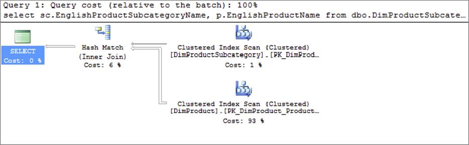
FIGURE 7-1

In SSIS, the data is usually joined using a Lookup Transformation on a buffered basis. The Merge Join Transformation can also be used, though it was designed to solve a different class of patterns. The calculus/algebra for these components is deterministic; the configuration that the user supplies is directly utilized by the engine — in other words, there is no opportunity for the platform to make any intelligent choices based on statistics, cost, cardinality, or count. Furthermore, the data is loaded into out-of-process buffers (with respect to the database engine) and is then treated on a row-by-row manner; therefore, because this moves the data away from the source, you can expect performance and scale to be affected.

Any data moving through an SSIS Data Flow is loaded into memory in data buffers. A batch process is performed on the data in synchronous transformations. The asynchronous transformations, such as the Sort or Aggregate, still perform in batch, but all rows must be loaded into memory before they complete, and therefore bring the pipeline process to a halt. Other transformations, like the OLE DB Command Transformation, perform their work using a row-by-row approach.

The end-user experience is synchronous, though in the case of some modes of the Lookup Transformation the process is blocked while the cache loads in its entirety. Execution is nonatomic in that one of multiple phases of the process can succeed or fail independently. Furthermore, you can direct successful matches to flow out the Lookup Transformation to one consumer, the nonmatches to flow to a separate consumer, and the errors to a third.

Resource usage and performance compete: in Lookup’s full-cache mode — which is typically fastest with smaller data sets — the cache is acquired and then remains in memory until the process (package) terminates, and there are no implicit operators (sorting, hashing, and paging) to balance resource usage. In no-cache or partial-cache modes, the resource usage is initially lower because the cache is charged on the fly; however, overall performance will almost always be lower. The operation is explicitly parallel; individual packages scale out if and only if the developer intentionally created multiple pipelines and manually segmented the data. Even then, bringing the data back together with the Union All Transformation, which is partial blocking, can negate any performance enhancement. Benchmark testing your SSIS packages is necessary to determine the best approach.

There is no opportunity for the Lookup Transformation to implicitly perform in an SMP (or scale-out) manner. The same applies to the Merge Join Transformation — on suitable hardware it will run on a separate thread to other components, but it will not utilize multiple threads within itself.

Figure 7-2 shows an SSIS package that uses a Lookup Transformation to demonstrate the same functionality as the previous SQL statement. Notice how the Product table is pipelined directly into the Lookup Transformation, but the SubCategory table is referenced using properties on the component itself. It is interesting to compare this package with the query plan generated by SQL Server for the previous SQL query. Notice how in this case SQL Server chose to utilize a hash-join operation, which happens to coincide with the mechanics underlying the Lookup Transformation when used in full-cache mode. The explicit design chosen by the developer in SSIS corresponds almost exactly to the plan chosen by SQL Server to generate the same result set.

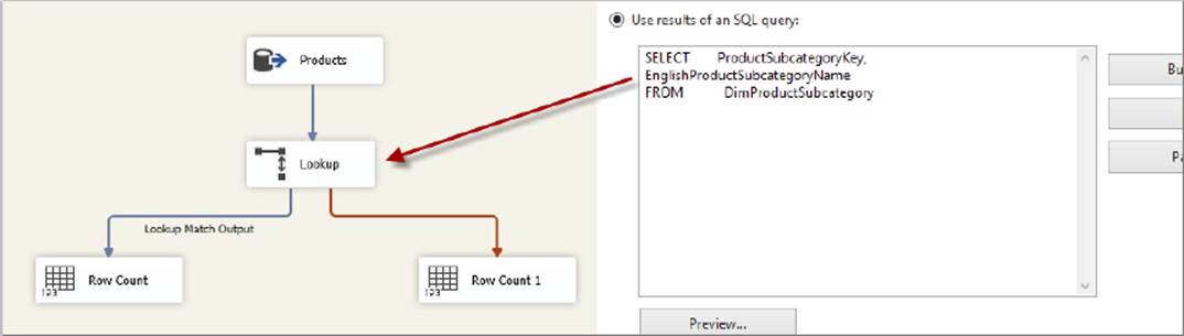
FIGURE 7-2

Figure 7-3 shows the same functionality, this time built using a Merge Join Transformation. Notice how similar this looks to the SQL Server plan (though in truth the execution semantics are quite different).

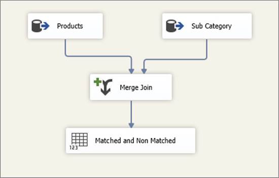
FIGURE 7-3

LOOKUP FEATURES

The Lookup Transformation allows you to populate the cache using a separate pipeline in either the same or a different package. You can use source data from any location that can be accessed by the SSIS Data Flow. This cache option makes it convenient to load a file or table into memory, and this data can be used by multiple Data Flows in multiple packages.

Prior to SQL Server 2008, you needed to reload the cache every time it was used. For example, if you had two Data Flow Tasks in the same package and each required the same reference data set, each Lookup Transformation would load its own copy of the cache separately. You can persist the cache to virtual memory or to permanent file storage. This means that within the same package, multiple Lookup Transformations can share the same cache. The cache does not need to be reloaded for multiple Data Flows or if the same Data Flow is executed multiple times during a package execution, such as when the Data Flow Task is executed within a Foreach Loop Container. You can also persist the cache to a file and share it with other packages. The cache file format is optimized for speed; it can be much faster than reloading the reference data set from the original relational source.

Another enhancement in the Lookup Transformation in SQL Server 2008 SSIS is the miss-cache feature. In scenarios where the component is configured to perform the Lookups directly against the database, the miss-cache feature enables you to optimize performance by optionally loading into cache the rows without matching entries in the reference data set. For example, if the component receives the value 123 in the incoming pipeline, but there are no matching entries in the reference data set, the component will not try to find that value in the reference data set again. In other words, the component “remembers” which values it did not find before. You can also specify how much memory the miss-cache should use (expressed as a percentage of the total cache limit, by default 20%). This reduces a redundant and expensive trip to the database. The miss-cache feature alone can contribute to performance improvement especially when you have a very large data set.

In the 2005 version of the component, the Lookup Transformation had only two outputs — one for matched rows and another that combined nonmatches and errors. However, the latter output caused much dismay with SSIS users — it is often the case that a nonmatch is not an error and is in fact expected. In 2008 and later the component has one output for nonmatches and a separate output for true errors (such as truncations). Note that the old combined output is still available as an option for backward compatibility. This combined error and nonmatching output can be separated by placing a Conditional Split Transformation after the Lookup, but it is no longer necessary because of the separate outputs.

To troubleshoot issues you may have with SSIS, you can add Data Viewers into a Data Flow on the lines connecting the components. Data Viewers give you a peek at the rows in memory. They also pause the Data Flow at the point the data reaches the viewer.

BUILDING THE BASIC PACKAGE

To simplify the explanation of the Lookup Transformation’s operation in the next few sections, this section presents a typical ETL problem that is used to demonstrate several solutions using the components configured in various modes.

The AdventureWorks database is a typical OLTP store for a bicycle retailer, and AdventureWorksDW is a database that contains the corresponding denormalized data warehouse structures. Both of these databases, as well as some secondary data, are used to represent a real-world ETL scenario. (If you do not have the databases, download them from www.wrox.com.)

The core operation focuses on extracting fact data from the source system (fact data is discussed in Chapter 12); in this scenario you will not yet be loading data into the warehouse itself. Obviously, you would not want to do one without the other in a real-world SSIS package, but it makes it easier to understand the solution if you tackle a smaller subset of the problem by itself.

You will first extract sales order (fact) data from the AdventureWorks, and later you will load it into the AdventureWorksDW database, performing multiple joins along the way. The order information in AdventureWorks is represented by two main tables: SalesOrderHeader and SalesOrderDetail. You need to join these two tables first.

The SalesOrderHeader table has many columns that in the real world would be interesting, but for this exercise you will scale down the columns to just the necessary few. Likewise, the SalesOrderDetail table has many useful columns, but you will use just a few of them. Here are the table structure and first five rows of data for these two tables:

As you can see, you need to join these two tables together because one table contains the order header information and the other contains the order details. Figure 7-4 shows a conceptual view of what the join would look like.

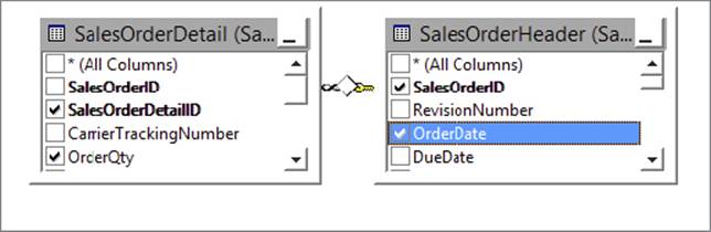
FIGURE 7-4

However, this does not get us all the way there. The CustomerID column is a surrogate key that is specific to the source system, and the very definition of surrogate keys dictates that no other system — including the data warehouse — should have any knowledge of them. Therefore, in order to populate the warehouse you need to get the original business (natural) key. Thus, you must join the SalesOrderHeader table (Sales.SalesOrderHeader) to the Customer table (Sales.Customer) in order to find the customer business key called AccountNumber. After doing that, your conceptual join now looks like Figure 7-5.

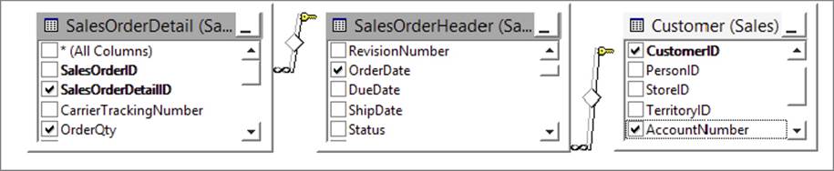
FIGURE 7-5

Similarly for Product, you need to add the Product table (Production.Product) to this join in order to derive the natural key called ProductNumber, as shown in Figure 7-6.

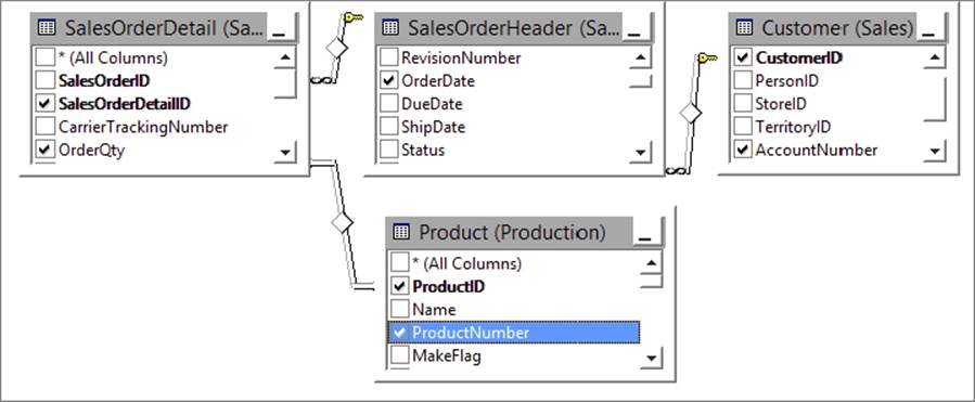
FIGURE 7-6

Referring to Figure 7-7, you can get started by creating a new SSIS package that contains an OLE DB Connection Manager called localhost.AdventureWorks that points to the AdventureWorks database and a single empty Data Flow Task.

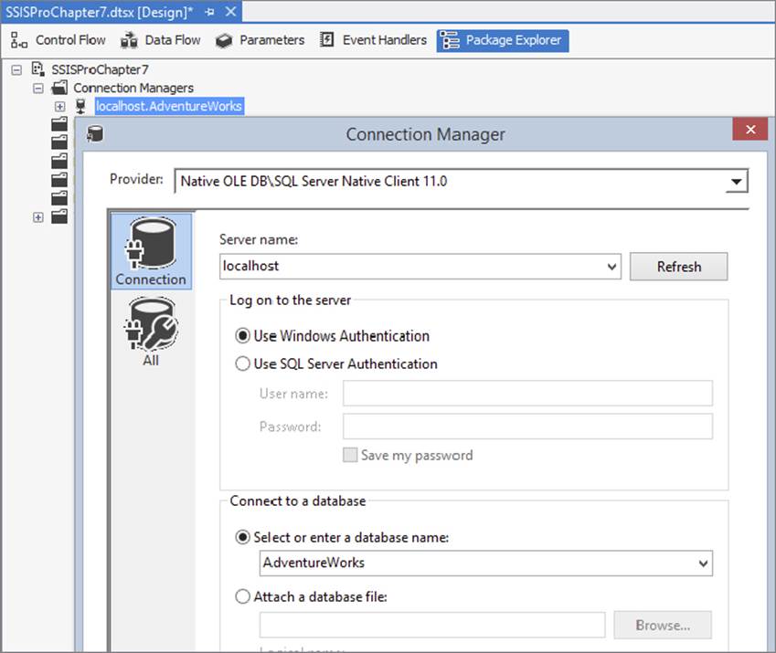
FIGURE 7-7

Using a Relational Join in the Source

The easiest and most obvious solution in this particular scenario is to use a relational join to extract the data. In other words, you can build a package that has a single source (use an OLE DB Source Component) and set the query string in the source to utilize relational joins. This enables you to take advantage of the benefits of the relational source database to prepare the data before it enters the SSIS Data Flow.

Drop an OLE DB Source Component on the Data Flow design surface, hook it up to the localhost. AdventureWorks Connection Manager, and set its query string as follows:

Select

--columns from Sales.SalesOrderHeader

oh.SalesOrderID, oh.OrderDate, oh.CustomerID,

--columns from Sales.Customer

c.AccountNumber,

--columns from Sales.SalesOrderDetail

od.SalesOrderDetailID, od.ProductID, od.OrderQty, od.UnitPrice, od.LineTotal,

--columns from Production.Product

p.ProductNumber

from Sales.SalesOrderHeader as oh

inner join Sales.Customer as c on (oh.CustomerID = c.CustomerID)

left join Sales.SalesOrderDetail as od on (oh.SalesOrderID = od.SalesOrderID)

inner join Production.Product as p on (od.ProductID = p.ProductID);

Note that you can either type this query in by hand or use the Build Query button in the user interface of the OLE DB Source Component to construct it visually. Click the Preview button and make sure that it executes correctly (see Figure 7-8).

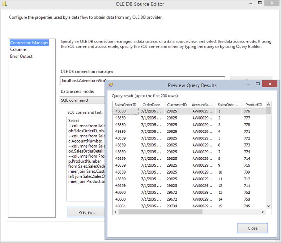
FIGURE 7-8

For seasoned SQL developers, the query should be fairly intuitive — the only thing worth calling out is that a left join is used between the SalesOrderHeader and SalesOrderDetail tables because it is conceivable that an order header could exist without any corresponding details. If an inner join was used here, it would have lost all such rows exhibiting this behavior. Conversely, inner joins were used everywhere else because an order header cannot exist without an associated customer, and a details row cannot exist without an associated product. In business terms, a customer will buy one or (hopefully) more products.

Close the preview dialog; click OK on the OLE DB Source Editor UI, and then hook up the Source Component to a Union All Transformation as shown in Figure 7-9, which serves as a temporary destination. Add a Data Viewer to the pipeline in order to watch the data travel through the system. Execute the package in debug mode and notice that the required results appear in the Data Viewer window.

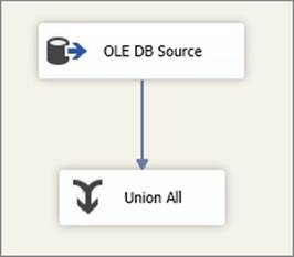
FIGURE 7-9

The Union All Transformation has nothing to do with this specific solution; it serves simply as a dead end in the Data Flow in order to get a temporary trash destination so that you don’t have to physically land the data in a database or file. This is a great way to test your Data Flows during development; placing a Data Viewer just before the Union All gives you a quick peek at the data. After development you would need to replace the Union All with a real destination. Note that you could also use some other component such as the Conditional Split. Keep in mind that some components, like the Row Count, require extra setup (such as variables), which would make this approach more cumbersome. Third-party tools are also available (such as Task Factory by Pragmatic Works) that have trash destinations for testing purposes only.

Using the Merge Join Transformation

Another way you could perform the join is to use Merge Join Transformations. In this specific scenario it does not make much sense because the database will likely perform the most optimal joins, as all the data resides in one place. However, consider a system in which the four tables you are joining reside in different locations; perhaps the sales and customer data is in SQL Server, and the product data is in a flat file, which is dumped nightly from a mainframe. The following steps explain how you can build a package to emulate such a scenario:

1. Start again with the basic package (refer to Figure 7-7) and proceed as follows. Because you do not have any actual text files as sources, you will create them inside the same package and then utilize them as needed. Of course, a real solution would not require this step; you just need to do this so that you can emulate a more complex scenario.

2. Name the empty Data Flow Task “DFT Create Text Files.” Inside this task create a pipeline that selects the required columns from the Product table in the AdventureWorks database and writes the data to a text file. Here is the SQL statement you will need:

3. select ProductID, ProductNumber

from Production.Product;

4. Connect the source to a Flat File destination and then configure the Flat File Destination Component to write to a location of your choice on your local hard drive, and make sure you select the delimited option and specify column headers when configuring the destination options, as shown in Figure 7-10. Name the flat file Product.txt.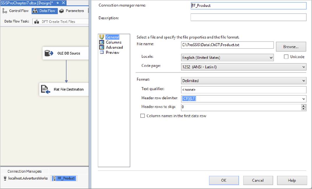

FIGURE 7-10

5. Execute the package to create a text file containing the Product data. Now create a second Data Flow Task and rename it “DFT Extract Source.” Connect the first and second Data Flow Tasks with a precedence constraint so that they execute serially, as shown inFigure 7-11. Inside the second (new) Data Flow Task, you’ll use the Lookup and Merge Join solutions to achieve the same result you did previously.

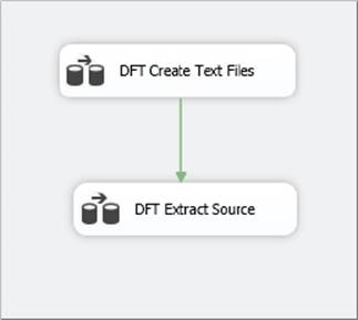
FIGURE 7-11

When using the Lookup Transformation, make sure that the largest table (usually a fact table) is streamed into the component, and the smallest table (usually a dimension table) is cached. That’s because the table that is cached will block the flow while it is loaded into memory, so you want to make sure it is as small as possible. Data Flow execution cannot begin until all Lookup data is loaded into memory. Since all of the data is loaded into memory, it makes the 3GB process limit on 32-bit systems a real challenge. In this case, all the tables are small, but imagine that the order header and details data is the largest, so you don’t want to incur the overhead of caching it. Thus, you can use a Merge Join Transformation instead of a Lookup to achieve the same result, without the overhead of caching a large amount of data. In some situations you can’t control the table’s server location, used in the Lookup, because the source data needs to run through multiple Lookups. A good example of this multiple Lookup Data Flow would be the loading of a fact table.

The simplest solution for retrieving the relational data would be to join the order header and order details tables directly in the Source Component (in a similar manner to that shown earlier). However, the following steps take a more complex route in order to illustrate some of the other options available:

1. Drop an OLE DB Source Component on the design surface of the second Data Flow Task and name it “SRC Order Header.” Hook it up to the AdventureWorks Connection Manager and use the following statement as the query:

2. select SalesOrderID, OrderDate, CustomerID

from Sales.SalesOrderHeader;

Of course, you could just choose the Table or View option in the source UI, or use a select* query, and perhaps even deselect specific columns in the Columns tab of the UI. However, these are all bad practices that will usually lead to degraded performance. It is imperative that, where possible, you specify the exact columns you require in the select clause. Furthermore, you should use a predicate (where clause) to limit the number of rows returned to just the ones you need.

3. Confirm that the query executes successfully by using the Preview button, and then hook up a Sort Transformation downstream of the source you have just created. Open the editor for the Sort Transformation and choose to sort the data by the SalesOrderID column, as shown in Figure 7-12. The reason you do this is because you will use a Merge Join Transformation later, and it requires sorted input streams. (Note that the Lookup Transformation does not require sorted inputs.) Also, an ORDER BY clause in the source would be better for performance, but this example is giving you experience with the Sort Transform.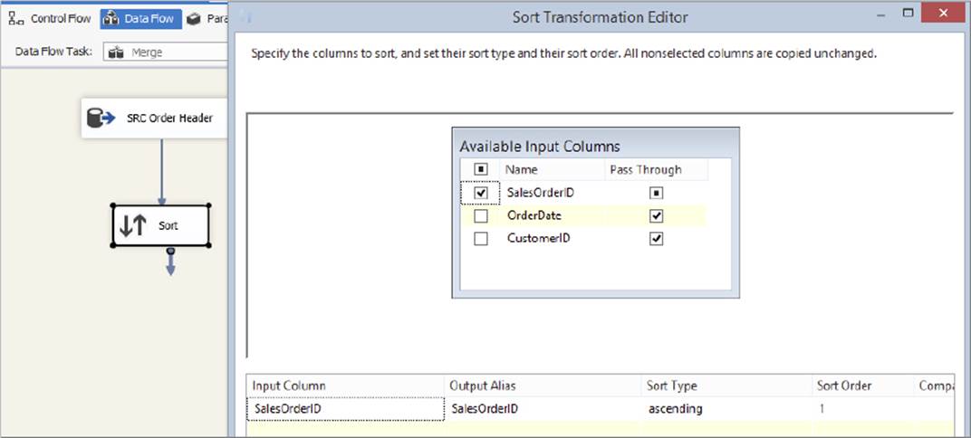

FIGURE 7-12

4. To retrieve the SalesOrderDetails data, drop another OLE DB Source Component on the design surface, name it SRC Details, and set its query as follows. Notice how in this case you have included an ORDER BY clause directly in the SQL select statement. This is more efficient than the way you sorted the order header data, because SQL Server can sort it for you before passing it out-of-process to SSIS. Again, you will see different methods to illustrate the various options available:

5. select SalesOrderID, SalesOrderDetailID, ProductID, OrderQty, UnitPrice,

6. LineTotal

7. from Sales.SalesOrderDetail

order by SalesOrderID, SalesOrderDetailID, ProductID;

8. Now drop a Merge Join Transformation on the surface and connect the outputs from the two Source Components to it. Specify the input coming from SRC Header (via the Sort Transformation) to be the left input, and the input coming from SRC Details to be the right input. You need to do this because, as discussed previously, you want to use a left join in order to keep rows from the header that do not have corresponding detail records.

After connecting both inputs, try to open the editor for the Merge Join Transformation; you should receive an error stating that “The IsSorted property must be set to True on both sources of this transformation.” The reason you get this error is because the Merge Join Transformation requires inputs that are sorted exactly the same way. However, you did ensure this by using a Sort Transformation on one stream and an explicit T-SQL ORDER BY clause on the other stream, so what’s going on? The simple answer is that the OLE DB Source Component works in a pass-through manner, so it doesn’t know that the ORDER BY clause was specified in the second SQL query statement due to the fact that the metadata returned by SQL Server includes column names, positions, and data types but does not include the sort order. By using the Sort Transformation, you forced SSIS to perform the sort, so it is fully aware of the ordering.

In order to remedy this situation, you have to tell the Source Transformation that its input data is presorted. Be very careful when doing this — by specifying the sort order in the following way, you are asking the system to trust that you know what you are talking about and that the data is in fact sorted. If the data is not sorted, or it is sorted other than the way you specified, then your package can act unpredictably, which could lead to data integrity issues and data loss. Use the following steps to specify the sort order:

1. Right-click the SRC Details Component and choose Show Advanced Editor. Select the Input and Output Properties tab, shown in Figure 7-13, and click the Root Node for the default output (not the error output). In the property grid on the right-hand side is a property called IsSorted. Change this to True.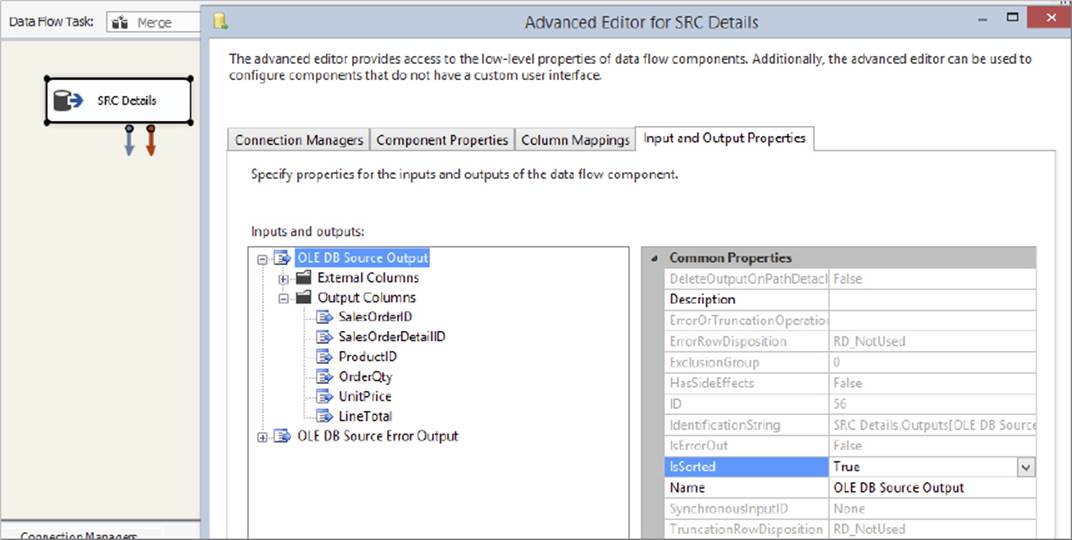

FIGURE 7-13

2. The preceding step tells the component that the data is presorted, but it does not indicate the order. Therefore, the next step is to select the columns that are being sorted on, and assign them values as follows:

· If the column is not sorted, then the value should be zero.

· If the column is sorted in ascending order, then the value should be positive.

· If the column is sorted in descending order, then the value should be negative.

The absolute value of the number should correspond to the column’s position in the order list. For instance, if the query was sorted as follows, “SalesOrderID ascending, ProductID descending,” then you would assign the value 1 to SalesOrderID and the value -2 to ProductID, with all other columns being 0.

3. Expand the Output Columns Node under the same default Output Node, and then select the SalesOrderID column. In the property grid, set the SortKeyPosition value to 1, as shown in Figure 7-14.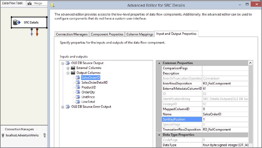

FIGURE 7-14

4. Close the dialog and try again to open the Merge Join UI; this time you should be successful. By default, the component works in inner join mode, but you can change that very easily by selecting (in this case) Left Outer Join from the Join type dropdown (seeFigure 7-15). You can also choose a Full Outer Join, which would perform a Cartesian join of all the data, though depending on the size of the source data, this will have a high memory overhead.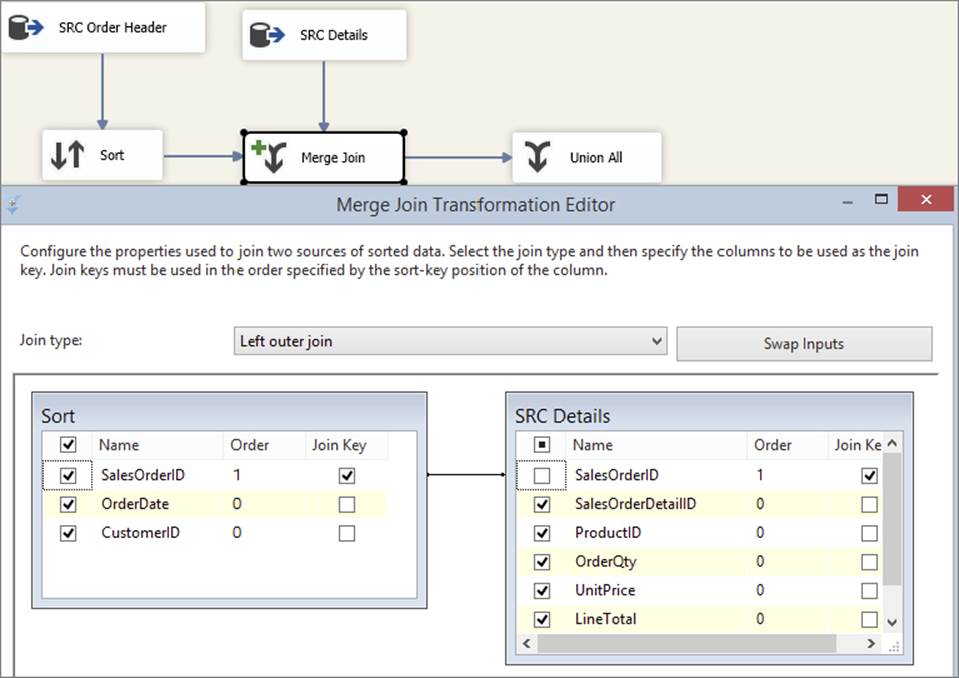

FIGURE 7-15

5. If you had made a mistake earlier while specifying which input was the left and which was the right, you can click the Swap Inputs button to switch their places. The component will automatically figure out which columns you are joining on based on their sort orders; if it gets it wrong, or there are more columns you need to join on, you can drag a column from the left to the right in order to specify more join criteria. However, the component will refuse any column combinations that are not part of the ordering criteria.

6. Finally, drop a Union All Transformation on the surface and connect the output of the Merge Join Transformation to it. Place a Data Viewer on the output path of the Merge Join Transformation and execute the package. Check the results in the Data Viewer; the data should be joined as required.

Merge Join is a useful component to use when memory limits or data size restricts you from using a Lookup Transformation. However, it requires the sorting of both input streams — which may be challenging to do with large data sets — and by design it does not provide any way of caching either data set. The next section examines the Lookup Transformation, which can help you solve join problems in a different way.

USING THE LOOKUP TRANSFORMATION

The Lookup Transformation solves join differently than the Merge Join Transformation. The Lookup Transformation typically caches one of the data sets in memory, and then compares each row arriving from the other data set in its input pipeline against the cache. The caching mechanism is highly configurable, providing a variety of different options in order to balance the performance and resource utilization of the process.

Full-Cache Mode

In full-cache mode, the Lookup Transformation stores all the rows resulting from a specified query in memory. The benefit of this mode is that Lookups against the in-memory cache are very fast — often an order of magnitude or more, relative to a no-cache mode Lookup. Full-cache mode is the default because in most scenarios it has the best performance of all of the techniques discussed in the chapter.

Continuing with the example package you built in the previous section (“Using the Merge Join Transformation”), you will in this section extend the existing package in order to join the other required tables. You already have the related values from the order header and order detail tables, but you still need to map the natural keys from the Product and Customer tables. You could use Merge Join Transformations again, but this example demonstrates how the Lookup Transformation can be of use here:

1. Open the package you created in the previous step. Remove the Union All Transformation. Drop a Lookup Transformation on the surface, name it LKP Customer, and connect the output of the Merge Join Transformation to it. Open the editor of the Lookup Transformation.

2. Select Full-Cache Mode, specifying an OLE DB Connection Manager. There is also an option to specify a Cache Connection Manager (CCM), but you won’t use this just yet — later in this chapter you will learn how to use the CCM. (After you have learned about the CCM, you can return to this exercise and try to use it here instead of the OLE DB Connection Manager.)

3. Click the Connection tab and select the AdventureWorks connection, and then use the following SQL query:

4. select CustomerID, AccountNumber

from Sales.Customer;

5. Preview the results to ensure that everything is set up OK, then click the Columns tab. Drag the CustomerID column from the left-hand table over to the CustomerID column on the right; this creates a linkage between these two columns, which tells the component that this column is used to perform the join. Click the checkbox next to the AccountNumber column on the right, which tells the component that you want to retrieve the AccountNumber values from the Customer table for each row it compares. Note that it is not necessary to retrieve the CustomerID values from the right-hand side because you already have them from the input columns. The editor should now look like Figure 7-16.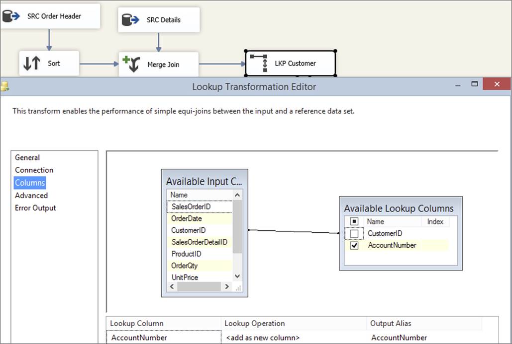

FIGURE 7-16

6. Click OK on the dialog, hook up a “trash” Union All Transformation (refer to Figure 7-9, choosing Lookup Match Output on the dialog that is invoked when you do this). Create a Data Viewer on the match output path of the Lookup Transformation and execute the package (you could also attach a Data Viewer on the no-match output and error output if needed). You should see results similar to Figure 7-17. Notice you have all the columns from the order and details data, as well as the selected column from the Customer table.

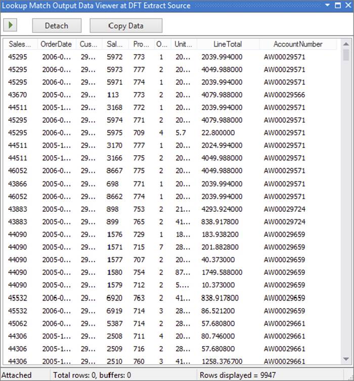
FIGURE 7-17

Because the Customer table is so small and the package runs so fast, you may not have noticed what happened here. As part of the pre-execution phase of the component, the Lookup Transformation fetched all the rows from the Customer table using the query specified (because the Lookup was configured to execute in full-cache mode). In this case there are only 20,000 or so rows, so this happens very quickly. Imagine that there were many more rows, perhaps two million. In this case you would likely experience a delay between executing the package and seeing any data actually traveling down the second pipeline.

Figure 7-18 shows a decision tree that demonstrates how the Lookup Transformation in full-cache mode operates at runtime. Note that the Lookup Transformation can be configured to send found and not-found rows to the same output, but the illustration assumes they are going to different outputs. In either case, the basic algorithm is the same.

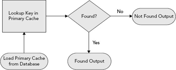
FIGURE 7-18

Check the Execution Results tab on the SSIS design surface (see Figure 7-19) and see how long it took for the data to be loaded into the in-memory cache. In larger data sets this number will be much larger and could even take longer than the execution of the primary functionality!

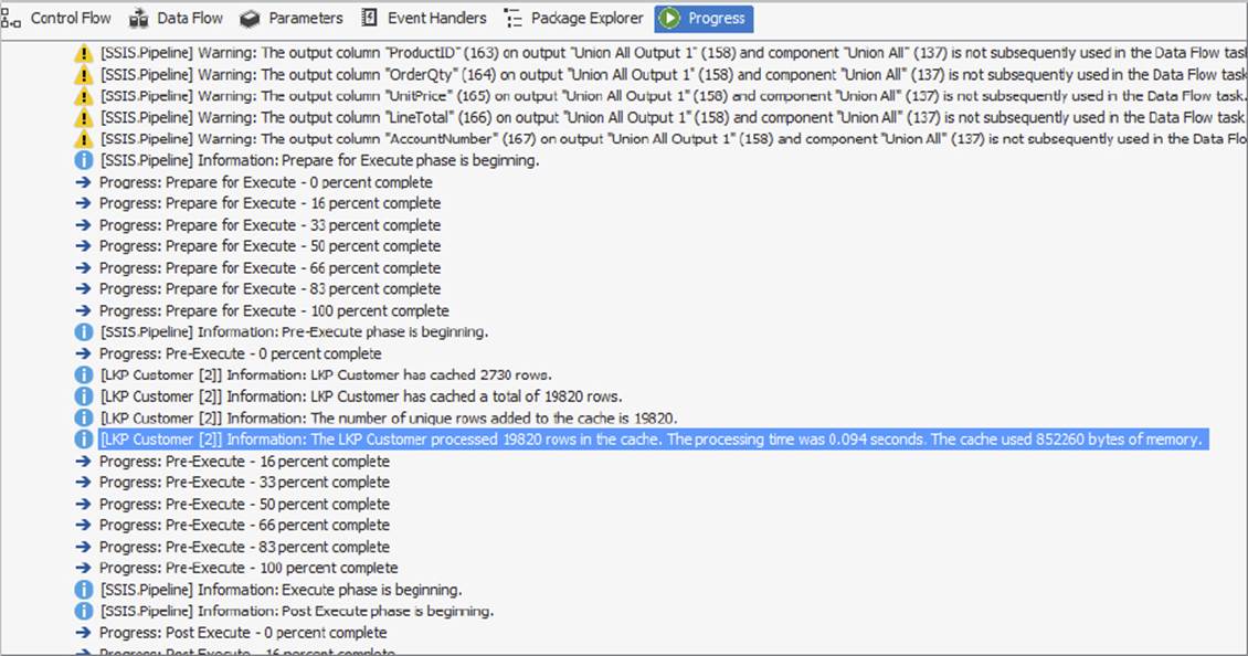
FIGURE 7-19

If during development and testing you want to emulate a long-running query, use the T-SQL waitfor statement in the query in the following manner.

waitfor delay '00:00:059'; --Wait 5 seconds before returning any

rows

select CustomerID, AccountNumber

from Sales.Customer;

After fetching all the rows from the specified source, the Lookup Transformation caches them in memory in a special hash structure. The package then continues execution; as each input row enters the Lookup Transformation, the specified key values are compared to the in-memory hash values, and, if a match is found, the specified return values are added to the output stream.

No-Cache Mode

If the reference table (the Customer table in this case) is too large to cache all at once in the system’s memory, you can choose to cache nothing or you can choose to cache only some of the data. This section explores the first option: no-cache mode.

In no-cache mode, the Lookup Transformation is configured almost exactly the same as in full-cache mode, but at execution time the reference table is not loaded into the hash structure. Instead, as each input row flows through the Lookup Transformation, the component sends a request to the reference table in the database server to ask for a match. As you would expect, this can have a high performance overhead on the system, so use this mode with care.

Depending on the size of the reference data, this mode is usually the slowest, though it scales to the largest number of reference rows. It is also useful for systems in which the reference data is highly volatile, such that any form of caching would render the results stale and erroneous.

Figure 7-20 illustrates the decision tree that the component uses during runtime. As before, the diagram assumes that separate outputs are configured for found and not-found rows, though the algorithm would be the same if all rows were sent to a single output.

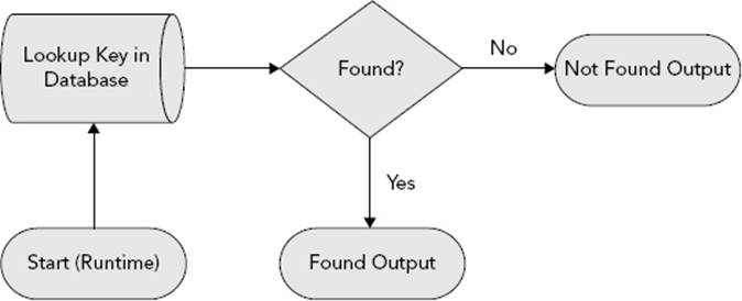
FIGURE 7-20

Here are the steps to build a package that uses no-cache mode:

1. Rather than build a brand-new package to try out no-cache mode, use the package you built in the previous section (“Full-Cache Mode”). Open the editor for the Lookup Transformation and on the first tab (General), choose the No-Cache option. This mode also enables you to customize (optimize) the query that SSIS will submit to the relational engine. To do this, click the Advanced tab and check the Modify the SQL Statement checkbox. In this case, the auto-generated statement is close enough to optimal, so you don’t need to touch it. (If you have any problems reconfiguring the Lookup Transformation, then delete the component, drop a new Lookup on the design surface, and reconnect and configure it from scratch.)

2. Execute the package. It should take slightly longer to execute than before, but the results should be the same.

The trade-off you make between the caching modes is one of performance versus resource utilization. Full-cache mode can potentially use a lot of memory to hold the reference rows in memory, but it is usually the fastest because Lookup operations do not require a trip to the database. No-cache mode, on the other hand, requires next to no memory, but it’s slower because it requires a database call for every Lookup. This is not a bad thing; if your reference table is volatile (i.e., the data changes often), you may want to use no-cache mode to ensure that you always have the latest version of each row.

Partial-Cache Mode

Partial-cache mode gives you a middle ground between the no-cache and full-cache options. In this mode, the component caches only the most recently used data within the memory boundaries specified under the Advanced tab in the Lookup Transform. As soon as the cache grows too big, the least-used cache data is thrown away.

When the package starts, much like in no-cache mode, no data is preloaded into the Lookup cache. As each input row enters the component, it uses the specified key(s) to attempt to find a matching record in the reference table using the specified query. If a match is found, then both the key and the Lookup values are added to the local cache on a just-in-time basis. If that same key enters the Lookup Transformation again, it can retrieve the matching value from the local cache instead of the reference table, thereby saving the expense and time incurred of requerying the database.

In the example scenario, for instance, suppose the input stream contains a CustomerID of 123. The first time the component sees this value, it goes to the database and tries to find it using the specified query. If it finds the value, it retrieves the AccountNumber and then adds the CustomerID/AccountNumber combination to its local cache. If CustomerCD 123 comes through again later, the component will retrieve the AccountNumber directly from the local cache instead of going to the database.

If, however, the key is not found in the local cache, the component will check the database to see if it exists there. Note that the key may not be in the local cache for several reasons: maybe it is the first time it was seen, maybe it was previously in the local cache but was evicted because of memory pressure, or finally, it could have been seen before but was also not found in the database.

For example, if CustomerID 456 enters the component, it will check the local cache for the value. Assuming it is not found, it will then check the database. If it finds it in the database, it will add 456 to its local cache. The next time CustomerID 456 enters the component, it can retrieve the value directly from its local cache without going to the database. However, it could also be the case that memory pressure caused this key/value to be dropped from the local cache, in which case the component will incur another database call.

If CustomerID 789 is not found in the local cache, and it is not subsequently found in the reference table, the component will treat the row as a nonmatch, and will send it down the output you have chosen for nonmatched rows (typically the no-match or error output). Every time that CustomerID 789 enters the component, it will go through these same set of operations. If you have a high degree of expected misses in your Lookup scenario, this latter behavior — though proper and expected — can be a cause of long execution times because database calls are expensive relative to a local cache check.

To avoid these repeated database calls while still getting the benefit of partial-cache mode, you can use another feature of the Lookup Transformation: the miss cache. Using the partial-cache and miss-cache options together, you can realize further performance gains. You can specify that the component remembers values that it did not previously find in the reference table, thereby avoiding the expense of looking for them again. This feature goes a long way toward solving the performance issues discussed in the previous paragraph, because ideally every key is looked for once — and only once — in the reference table.

To configure this mode, follow these steps (refer to Figure 7-21):

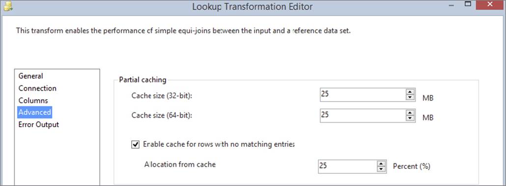
FIGURE 7-21

1. Open the Lookup editor, and in the General tab select the Partial Cache option. In the Advanced tab, specify the upper memory boundaries for the cache and edit the SQL statement as necessary. Note that both 32-bit and 64-bit boundaries are available because the package may be built and tested on a 32-bit platform but deployed to a 64-bit platform, which has more memory. Providing both options makes it simple to configure the component’s behavior on both platforms.

2. If you want to use the miss-cache feature, configure what percentage of the total cache memory you want to use for this secondary cache (say, 25%).

The decision tree shown in Figure 7-22 demonstrates how the Lookup Transformation operates at runtime when using the partial-cache and miss-cache options. Note that some of the steps are conceptual; in reality, they are implemented using a more optimal design. As per the decision trees shown for the other modes, this illustration assumes separate outputs are used for the found and not-found rows.

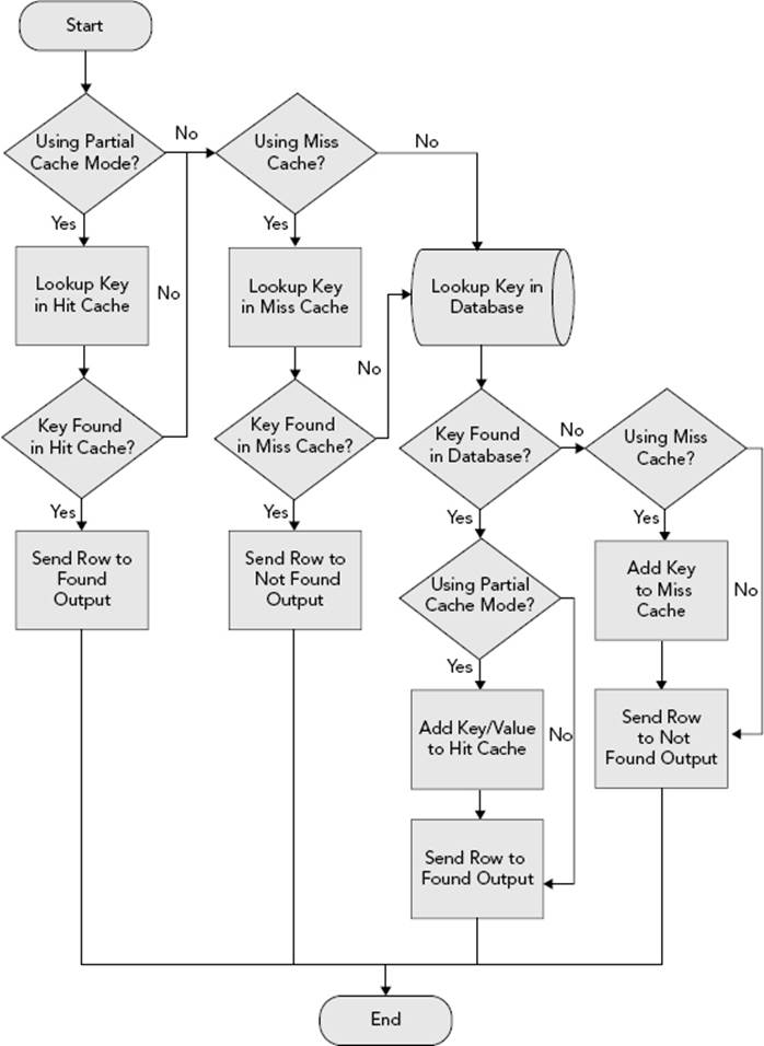
FIGURE 7-22

Multiple Outputs

At this point, your Lookup Transformation is working, and you have learned different ways to optimize its performance using fewer or more resources. In this section, you’ll learn how to utilize some of the other features in the component, such as the different outputs that are available.

Using the same package you built in the previous sections, follow these steps:

1. Reset the Lookup Transformation so that it works in full-cache mode. It so happens that, in this example, the data is clean and thus every row finds a match, but you can emulate rows not being found by playing quick and dirty with the Lookup query string. This is a useful trick to use at design time in order to test the robustness and behavior of your Lookup Transformations. Change the query statement in the Lookup Transformation as follows:

2. select CustomerID, AccountNumber

3. from Sales.Customer

where CustomerID % 7 <> 0; --Remove 1/7 of the rows

4. Run the package again. This time, it should fail to execute fully because the cache contains one-seventh fewer rows than before, so some of the incoming keys will not find a match, as shown in Figure 7-23. Because the default error behavior of the component is to fail on any nonmatch or error condition such as truncation, the Lookup halts as expected.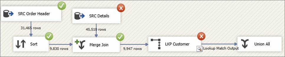

FIGURE 7-23

Try some of the other output options. Open the Lookup editor and on the dropdown listbox in the General tab, choose how you want the Lookup Transformation to behave when it does not manage to find a matching join entry:

· Fail Component should already be selected. This is the default behavior, which causes the component to raise an exception and halt execution if a nonmatching row is found or a row causes an error such as data truncation.

· Ignore Failure sends any nonmatched rows and rows that cause errors down the same output as the matched rows, but the Lookup values (in this case AccountNumber) will be set to null. If you add a Data Viewer to the flow, you should be able to see this; several of the AccountNumbers will have null values.

· Redirect Rows to Error Output is provided for backward compatibility with SQL Server 2005. It causes the component to send both nonmatched and error-causing rows down the same error (red) output.

· Redirect Rows to No Match Output causes errors to flow down the error (red) output, and no-match rows to flow down the no-match output.

5. Choose Ignore Failure and execute the package. The results should look like Figure 7-24. You can see that the number of incoming rows on the Lookup Transformation matches the number of rows coming out of its match output, even though one-seventh of the rows were not actually matched. This is because the rows failed to find a match, but because you configured the Ignore Failure option, the component did not stop execution.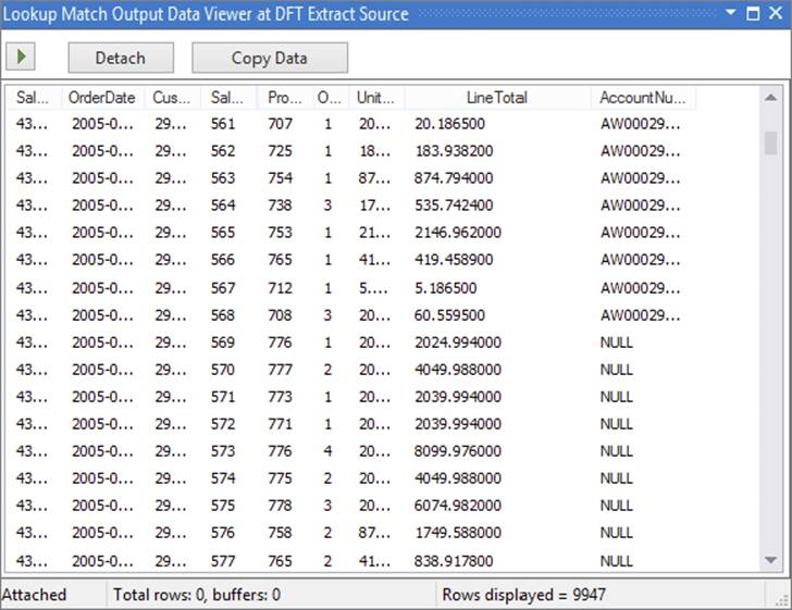

FIGURE 7-24

6. Open the Lookup Transformation and this time select “Redirect rows to error output.” In order to make this option work, you need a second trash destination on the error output of the Lookup Transformation, as shown in Figure 7-25. When you execute the package using this mode, the found rows will be sent down the match output, and unlike the previous modes, not-found rows will not be ignored or cause the component to fail but will instead be sent down the error output.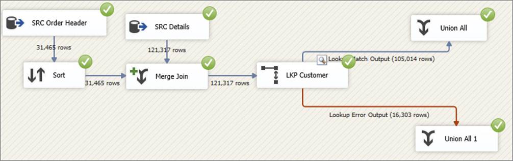

FIGURE 7-25

7. Finally, test the “Redirect rows to no match output” mode. You will need a total of three trash destinations for this to work, as shown in Figure 7-26.

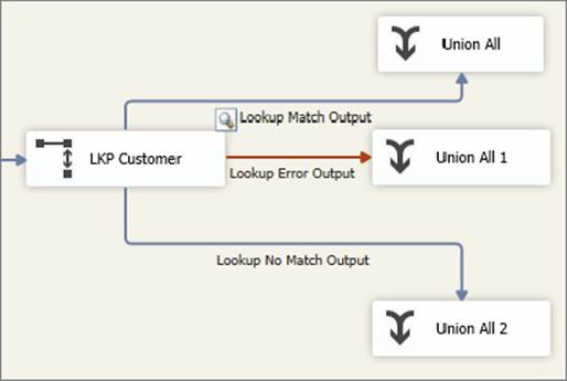
FIGURE 7-26

In all cases, add Data Viewers to each output, execute the package, and examine the results. The outputs should not contain any errors such as truncations, though there should be many nonmatched rows.

So how exactly are these outputs useful? What can you do with them to make your packages more robust? In most cases, the errors or nonmatched rows can be piped off to a different area of the package where the values can be logged or fixed as per the business requirements. For example, one common solution is for all missing rows to be tagged with an Unknown member value. In this scenario, all nonmatched rows might have their AccountNumber set to 0000. These fixed values are then joined back into the main Data Flow and from there treated the same as the rows that did find a match. Use the following steps to configure the package to do this:

1. Open the Lookup editor. On the General tab, choose the “Redirect rows to no match output” option. Click the Error Output tab (see Figure 7-27) and configure the AccountNumber column to have the value Fail Component under the Truncation column. This combination of settings means that you want a no-match output, but you don’t want an error output; instead you want the component to fail on any errors. In a real-world scenario, you may want to have an error output that you can use to log values to an error table, but this example keeps it simple.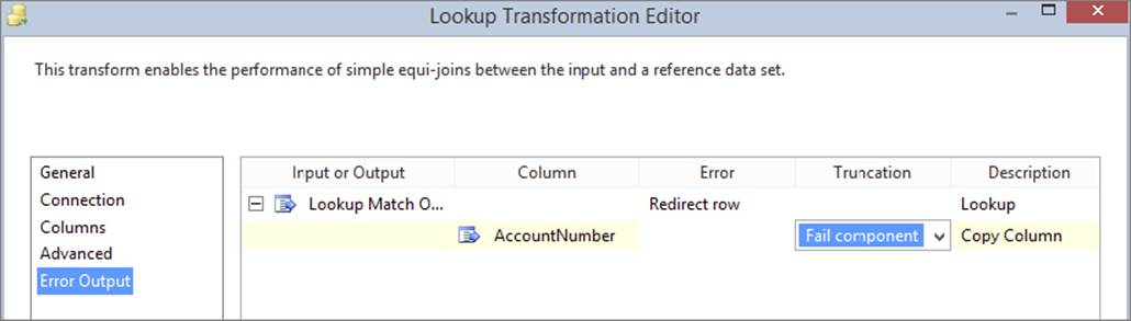

FIGURE 7-27

2. At this point, you could drop a Derived Column Transformation on the design surface and connect the no-match output to it. Then you would add the AccountNumber column in the derived column, and use a Union All to bring the data back together. This approach works, but the partially blocking Union All slows down performance.

However, there is a better way to design the Data Flow. Set the Lookup to Ignore Errors. Drop a Derived Column on the Data Flow. Connect the match output to the derived column. Open the Derived Column editor and replace the AccountNumber column with the following expression (see Chapter 5 for more details).

ISNULL(AccountNumber)?(DT_STR,10,1252)"0000":AccountNumber

The Derived Column Transformation dialog editor should now look something like Figure 7-28.

FIGURE 7-28

Close the Derived Column editor, and drop a Union All Transformation on the surface. Connect the default output from the Derived Column to the Union All Transformation and then execute the package, as usual utilizing a Data Viewer on the final output. The package and results should look something like Figure 7-29.

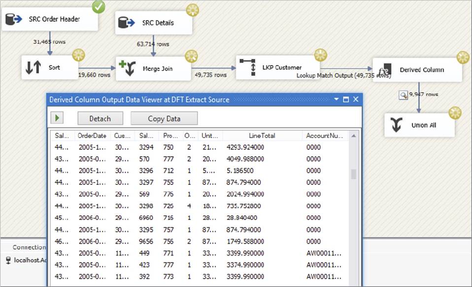
FIGURE 7-29

The output should show AccountNumbers for most of the values, with 0000 shown for those keys that are not present in the reference query (in this case because you artificially removed them).

Expressionable Properties

If you need to build a package whose required reference table is not known at design time, this feature will be useful for you. Instead of using a static query in the Lookup Transformation, you can use an expression, which can dynamically construct the query string, or it could load the query string using the parameters feature. Parameters are discussed in Chapter 5 and Chapter 22.

Figure 7-30 shows an example of using an expression within a Lookup Transformation. Expressions on Data Flow Components can be accessed from the property page of the Data Flow Task itself. See Chapter 5 for more details.

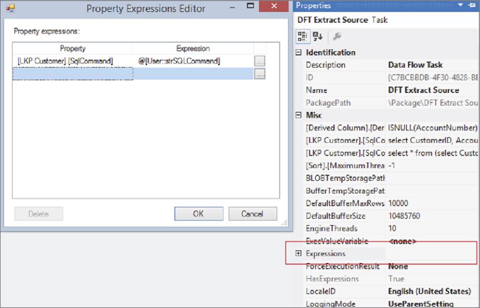
FIGURE 7-30

Cascaded Lookup Operations

Sometimes the requirements of a real-world Data Flow may require several Lookup Transformations to get the job done. By using multiple Lookup Transformations, you can sometimes achieve a higher degree of performance without incurring the associated memory costs and processing times of using a single Lookup.

Imagine you have a large list of products that ideally you would like to load into one Lookup. You consider using full-cache mode; however, because of the sheer number of rows, either you run out of memory when trying to load the cache or the cache-loading phase takes so long that it becomes impractical (for instance, the package takes 15 minutes to execute, but 6 minutes of that time is spent just loading the Lookup cache). Therefore, you consider no-cache mode, but the expense of all those database calls makes the solution too slow. Finally, you consider partial-cache mode, but again the expense of the initial database calls (before the internal cache is populated with enough data to be useful) is too high.

The solution to this problem is based on a critical assumption that there is a subset of reference rows (in this case product rows) that are statistically likely to be found in most, if not all, data loads. For instance, if the business is a consumer goods chain, then it’s likely that a high proportion of sales transactions are from people who buy milk. Similarly, there will be many transactions for sales of bread, cheese, beer, and baby diapers. On the contrary, there will be a relatively low number of sales for expensive wines. Some of these trends may be seasonal — more suntan lotion sold in summer, and more heaters sold in winter. This same assumption applies to other dimensions besides products — for instance, a company specializing in direct sales may know historically which customers (or customer segments or loyalty members) have responded to specific campaigns. A bank might know which accounts (or account types) have the most activity at specific times of the month.

This statistical property does not hold true for all data sets, but if it does, you may derive great benefit from this pattern. If it doesn’t, you may still find this section useful as you consider the different ways of approaching a problem and solving it with SSIS.

So how do you use this statistical approach to build your solution? Using the consumer goods example, if it is the middle of winter and you know you are not going to be selling much suntan lotion, then why load the suntan products in the Lookup Transformation? Rather, load just the high-frequency items like milk, bread, and cheese. Because you know you will see those items often, you want to put them in a Lookup Transformation configured in full-cache mode. If your Product table has, say, 1 million items, then you could load the top 20% of them (in terms of frequency/popularity) into this first Lookup. That way, you don’t spend too much time loading the cache (because it is only 200,000 rows and not 1,000,000); by the same reasoning, you don’t use as much memory.

Of course, in any statistical approach there will always be outliers — for instance, in the previous example suntan lotion will still be sold in winter to people going on holiday to sunnier places. Therefore, if any Lookups fail on the first full-cache Lookup, you need a second Lookup to pick up the strays. The second Lookup would be configured in partial-cache mode (as detailed earlier in this chapter), which means it would make database calls in the event that the item was not found in its dynamically growing internal cache. The first Lookup’s not-found output would be connected to the second Lookup’s input, and both of the Lookups would have their found outputs combined using a Union All Transformation in order to send all the matches downstream. Then a third Lookup is used in no-cache mode to look up any remaining rows not found already. This final Lookup output is combined with the others in another Union All. Figure 7-31 shows what such a package might look like.

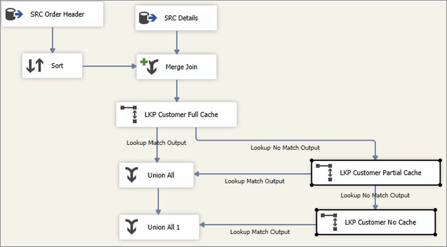
FIGURE 7-31

The benefit of this approach is that at the expense of a little more development time, you now have a system that performs efficiently for the most common Lookups and fails over to a slower mode for those items that are less common. That means that the Lookup operation will be extremely efficient for most of your data, which typically results in an overall decrease in processing time.

In other words, you have used the Pareto principle (80/20 rule) to improve the solution. The first (full-cache) Lookup stores 20% of the reference (in this case product) rows and hopefully succeeds in answering 80% of the Lookup requests. This is largely dependent on the user creating the right query to get the proper 20%. If the wrong data is queried then this can be a worst approach. For the 20% of Lookups that fail, they are redirected to — and serviced by — the partial-cache Lookup, which operates against the other 80% of data. Because you are constraining the size of the partial cache, you can ensure you don’t run into any memory limitations — at the extreme, you could even use a no-cache Lookup instead of, or in addition to, the partial-cache Lookup.

The final piece to this puzzle is how you identify up front which items occur the most frequently in your domain. If the business does not already keep track of this information, you can derive it by collecting statistics within your packages and saving the results to a temporary location. For instance, each time you load your sales data, you could aggregate the number of sales for each item and write the results to a new table you have created for that purpose. The next time you load the product Lookup Transformation, you join the full Product table to the statistics table and return only those rows whose aggregate count is above a certain threshold. (You could also use the data-mining functionality in SQL Server to derive this information, though the details of that are beyond the scope of this chapter.)

CACHE CONNECTION MANAGER AND CACHE TRANSFORM

The Cache Connection Manager (CCM) and Cache Transform enable you to load the Lookup cache from any source. The Cache Connection Manager is the more critical of the two components — it holds a reference to the internal memory cache and can both read and write the cache to a disk-based file. In fact, the Lookup Transformation internally uses the CCM as its caching mechanism.

Like other Connection Managers in SSIS, the CCM is instantiated in the Connection Managers pane of the package design surface. You can also create new CCMs from the Cache Transformation Editor and Lookup Transformation Editor. At design time, the CCM contains no data, so at runtime you need to populate it. You can do this in one of two ways:

· You can create a separate Data Flow Task within the same package to extract data from any source and load the data into a Cache Transformation, as shown in Figure 7-32. You then configure the Cache Transformation to write the data to the CCM. Optionally, you can configure the same CCM to write the data to a cache file (usually with the extension .caw) on disk. When you execute the package, the Source Component will send the rows down the pipeline into the input of the Cache Transformation. The Cache Transformation will call the CCM, which loads the data into a local memory cache. If configured, the CCM will also save the cache to disk so you can use it again later. This method enables you to create persisted caches that you can share with other users, solutions, and packages.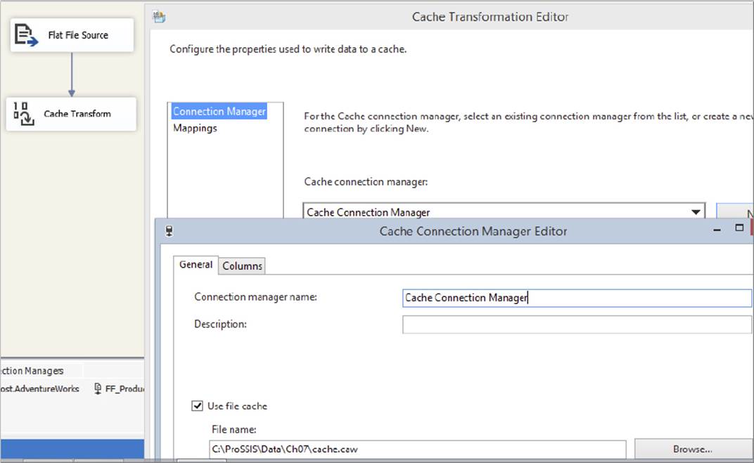

FIGURE 7-32

· Alternatively, you can open up the CCM editor and directly specify the filename of an existing cache file (.caw file). This option requires that a cache file has previously been created for you to reuse. At execution time, the CCM loads the cache directly from disk and populates its internal memory structures.

When you configure a CCM, you can specify which columns of the input data set should be used as index fields and which columns should be used as reference fields (see Figure 7-33). This is a necessary step — the CCM needs to know up front which columns you will be joining on, so that it can create internal index structures to optimize the process.

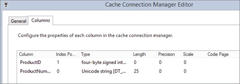
FIGURE 7-33

Whichever way you created the CCM, when you execute the package, the CCM will contain an in-memory representation of the data you specified. That means that the cache is now immediately available for use by the Lookup Transformation. Note that the Lookup Transformation is the only component that uses the caching aspects of the CCM; however, the Raw File Source can also read .caw files, which can be useful for debugging.

If you are using the Lookup Transformation in full-cache mode, you can load the cache using the CCM (instead of specifying a SQL query as described earlier in this chapter). To use the CCM option, open the Lookup Transformation and select Full Cache and Cache Connection Manager in the general pane of the editor, as shown in Figure 7-34. Then you can either select an existing CCM or create a new one. You can now continue configuring the Lookup Transformation in the same way you would if you had used a SQL query. The only difference is that in the Columns tab, you can only join on columns that you earlier specified as index columns in the CCM editor.

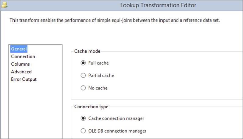
FIGURE 7-34

The CCM gives you several benefits. First of all, you can reuse caches that you previously saved to file (in the same or a different package). For instance, you can load a CCM using the Customer table and then save the cache to a .caw file on disk. Every other package that needs to do a Lookup against customers can then use a Lookup Transformation configured in full-cache/CCM mode, with the CCM pointing at the .caw file you created.

Second, reading data from a .caw file is generally faster than reading from OLE DB, so your packages should run faster. Of course, because the .caw file is an offline copy of your source data, it can become stale; therefore, it should be reloaded every so often. Note that you can use an expression for the CCM filename, which means that you can dynamically load specific files at runtime.

Third, the CCM enables you to reuse caches across loop iterations. If you use a Lookup Transformation in full-cache/OLE DB mode within an SSIS For Loop Container or Foreach Loop Container, the cache will be reloaded on every iteration of the loop. This may be your intended design, but if not, then it is difficult to mitigate the performance overhead. However, if you used a Lookup configured in full-cache/CCM mode, the CCM would be persistent across loop iterations, improving your overall package performance.

SUMMARY

This chapter explored different ways of joining data within an SSIS solution. Relational databases are highly efficient at joining data within their own stores; however, you may not be fortunate enough to have all your data living in the same database — for example, when loading a data warehouse. SSIS enables you to perform these joins outside the database and provides many different options for doing so, each with different performance and resource-usage characteristics.

The Merge Join Transformation can join large volumes of data without much memory impact; however, it has certain requirements, such as sorted input columns, that may be difficult to meet. Remember to use the source query to sort the input data, and avoid the Sort Transformation when possible, because of performance issues.

The Lookup Transformation is very flexible and supports multiple modes of operation. The Cache Connection Manager adds more flexibility to the Lookup by allowing caches to be explicitly shared across Data Flows and packages. With the CCM, the Lookup cache is also maintained across loop iterations. In large-scale deployments, many different patterns can be used to optimize performance, one of them being cascaded Lookups.

As with all SSIS solutions, there are no hard-and-fast rules that apply to all situations, so don’t be afraid to experiment. If you run into any performance issues when trying to join data, try a few of the other options presented in this chapter. Hopefully, you will find one that makes a difference.