Agile Data Science (2014)

Part I. Setup

Chapter 3. Agile Tools

This chapter will briefly introduce our software stack. This stack is optimized for our process. By the end of this chapter, you’ll be collecting, storing, processing, publishing, and decorating data. Our stack enables one person to do all of this, to go “full stack.” We’ll cover a lot, and quickly, but don’t worry: I will continue to demonstrate this software stack in Chapters 5 through 10. You need only understand the basics now; you will get more comfortable later.

We begin with instructions for running our stack in local mode on your own machine. In the next chapter, you’ll learn how to scale this same stack in the cloud via Amazon Web Services. Let’s get started.

Code examples for this chapter are available at https://github.com/rjurney/Agile_Data_Code/tree/master/ch03. Clone the repository and follow along!

git clone https://github.com/rujrney/Agile_Data_Code.git

Scalability = Simplicity

As NoSQL tools like Hadoop, MongoDB, data science, and big data have developed, much focus has been placed on the plumbing of analytics applications. This book teaches you to build applications that use such infrastructure. We will take this plumbing for granted and build applications that depend on it. Thus, this book devotes only two chapters to infrastructure: one on introducing our development tools, and the other on scaling them up in the cloud to match our data’s scale.

In choosing our tools, we seek linear scalability, but above all, we seek simplicity. While the concurrent systems required to drive a modern analytics application at any kind of scale are complex, we still need to be able to focus on the task at hand: processing data to create value for the user. When our tools are too complex, we start to focus on the tools themselves, and not on our data, our users, and new applications to help them. An effective stack enables collaboration by teams that include diverse sets of skills such as design and application development, statistics, machine learning, and distributed systems.

NOTE

The stack outlined in this book is not definitive. It has been selected as an example of the kind of end-to-end setup you should expect as a developer or should aim for as a platform engineer in order to rapidly and effectively build analytics applications. The takeaway should be an example stack you can use to jumpstart your application, and a standard to which you should hold other stacks.

Agile Big Data Processing

The first step to building analytics applications is to plumb your application from end to end: from collecting raw data to displaying something on the user’s screen (see Figure 3-1). This is important, because complexity can increase fast, and you need user feedback plugged into the process from the start, lest you start iterating without feedback (also known as the death spiral).

Events -> Collectors -> Bulk Storage -> Batch Processing -> Distributed Store -> Application Server -> Browser -> User

Figure 3-1. Flow of data processing in Agile Big Data

The components of our stack are thus:

§ Events are the things logs represent. An event is an occurrence that happens and is logged along with its features and timestamps.

Events come in many forms—logs from servers, sensors, financial transactions, or actions our users take in our own application. To facilitate data exchange among different tools and languages, events are serialized in a common, agreed-upon format.

§ Collectors are event aggregators. They collect events from numerous sources and log them in aggregate to bulk storage, or queue them for action by sub-real-time workers.

§ Bulk storage is a filesystem capable of parallel access by many concurrent processes. We’ll be using S3 in place of the Hadoop Distributed FileSystem (HDFS) for this purpose. HDFS sets the standard for bulk storage, and without it, big data would not exist. There would be no cheap place to store vast amounts of data where it can be accessed with high I/O throughput for the kind of processing we do in Agile Big Data.

§ Distributed document stores are multinode stores using document format. In Agile Big Data, we use them to publish data for consumption by web applications and other services. We’ll be using MongoDB as our distributed document store.

§ A minimalist web application server enables us to plumb our data as JSON through to the client for visualization, with minimal overhead. We use Python/Flask. Other examples are Ruby/Sinatra or Node.js.

§ A modern browser or mobile application enables us to present our data as an interactive experience for our users, who provide data through interaction and events describing those actions. In this book, we focus on web applications.

This list may look daunting, but in practice, these tools are easy to set up and match the crunch points in data science. This setup scales easily and is optimized for analytic processing.

Setting Up a Virtual Environment for Python

In this book, we use Python 2.7, which may or may not be the version you normally use. For this reason, we’ll be using a virtual environment (venv). To set up venv, install the virtualenv package.

With pip:

pip install virtualenv

With easy_install:

easy_install virtualenv

I have already created a venv environment in GitHub. Activate it via:

source venv/bin/activate

If, for some reason, the included venv does not work, then set up your virtual environment as follows:

virtualenv -p `which python2.7` venv --distribute

source venv/bin/activate

Now you can run pip install -r requirements.txt to install all required packages, and they will build under the venv/ directory.

To exit your virtual environment:

deactivate

Serializing Events with Avro

In our stack, we use a serialization system called Avro (see Figure 3-2). Avro allows us to access our data in a common format across languages and tools.

Events

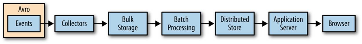
Figure 3-2. Serializing events

Avro for Python

Installation

To install Avro for Python, you must first build and install the snappy compression library, available at http://code.google.com/p/snappy/. Using a package manager to do so is recommended. Then install python-snappy via easy_install, pip, or from the source athttps://github.com/andrix/python-snappy. With python-snappy installed, Avro for Python should install without problems.

To install the Python Avro client from source:

[bash]$ git clone https://github.com/apache/avro.git

[bash]$ cd avro/lang/py

[bash]$ python setup.py install

To install using pip or easy_install:

pip install avro

easy_install avro

Testing

Try writing and reading a simple schema to verify that our data works (see Example 3-1):

[bash]$ python

Example 3-1. Writing avros in python (ch03/python/test_avro.py)

# Derived from the helpful example at

http://www.harshj.com/2010/04/25/writing-and-reading-avro-data-files-using-python/

fromavroimport schema, datafile, io

importpprint

OUTFILE_NAME = '/tmp/messages.avro'

SCHEMA_STR = """{

"type": "record",

"name": "Message",

"fields" : [

{"name": "message_id", "type": "int"},

{"name": "topic", "type": "string"},

{"name": "user_id", "type": "int"}

]

}"""

SCHEMA = schema.parse(SCHEMA_STR)

# Create a 'record' (datum) writer

rec_writer = io.DatumWriter(SCHEMA)

# Create a 'data file' (avro file) writer

df_writer = datafile.DataFileWriter(

open(OUTFILE_NAME, 'wb'),

rec_writer,

writers_schema = SCHEMA

)

df_writer.append( {"message_id": 11, "topic": "Hello galaxy", "user_id": 1} )

df_writer.append( {"message_id": 12, "topic": "Jim is silly!", "user_id": 1} )

df_writer.append( {"message_id": 23, "topic": "I like apples.", "user_id": 2} )

df_writer.close()

Verify that the messages are present:

[bash]$ ls -lah /tmp/messages.avro

-rw-r--r-- 1 rjurney wheel 263B Jan 23 17:30 /tmp/messages.avro

Now verify that we can read records back (Example 3-2).

Example 3-2. Reading avros in Python (ch03/python/test_avro.py)

fromavroimport schema, datafile, io

importpprint

# Test reading avros

rec_reader = io.DatumReader()

# Create a 'data file' (avro file) reader

df_reader = datafile.DataFileReader(

open(OUTFILE_NAME),

rec_reader

)

# Read all records stored inside

pp = pprint.PrettyPrinter()

for record indf_reader:

pp.pprint(record)

The output should look like this:

{u'message_id': 11, u'topic': u'Hello galaxy', u'user_id': 1}

{u'message_id': 12, u'topic': u'Jim is silly!', u'user_id': 1}

{u'message_id': 23, u'topic': u'I like apples.', u'user_id': 2}

Collecting Data

We’ll be collecting your own email via IMAP, as shown in Figure 3-3, and storing it to disk with Avro (Figure 3-3). Email conforms to a well-known schema defined in RFC-2822. We’ll use a simple utility to encapsulate the complexity of this operation. If an error or a slow Internet connection prevents you from downloading your entire inbox, that’s OK. You only need a few megabytes of data to work the examples, although more data makes the examples richer and more rewarding.

Collecting Data

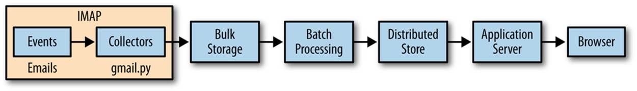
Figure 3-3. Collecting data via IMAP

Example 3-3. Avro schema for email (ch03/gmail/email.avro.schema)

{

"type":"record",

"name":"Email",

"fields":[

{ "name":"message_id", "type":["null","string"] },

{ "name":"thread_id", "type":["null","string"] },

{ "name":"in_reply_to","type":["string","null"] },

{ "name":"subject", "type":["string","null"] },

{ "name":"body", "type":["string","null"] },

{ "name":"date", "type":["string","null"] },

{

"name":"from",

"type":

{

"type":"record","name":"from",

"fields":[

{ "name":"real_name", "type":["null","string"] },

{ "name":"address", "type":["null","string"] }

] }

{

"name":"tos",

"type":[

"null",

{

"type":"array",

"items":[

"null",

{

"type":"record","name":"to",

"fields":[

{ "name":"real_name", "type":["null","string"] },

{ "name":"address", "type":["null","string"] }

] } ] } ]

{

"name":"ccs",

"type":[

"null",

{

"type":"array",

"items":[

"null",

{

"type":"record","name":"cc",

"fields":[

{ "name":"real_name", "type":["null","string"] },

{ "name":"address", "type":["null","string"] }

] } ] } ]

{

"name":"bccs",

"type":[

"null",

{

"type":"array",

"items":[

"null",

{

"type":"record","name":"bcc",

"fields":[

{ "name":"real_name", "type":["null","string"] },

{ "name":"address", "type":["null","string"] }

] } ] } ]

{

"name":"reply_tos",

"type":[

"null",

{

"type":"array",

"items":[

"null",

{

"type":"record","name":"reply_to",

"fields":[

{ "name":"real_name", "type":["null","string"] },

{ "name":"address", "type":["null","string"] }

] } ] } ] }

]

}

Python’s imaplib makes connecting to Gmail easy, as shown in Example 3-4.

Example 3-4. Scraping IMAP with gmail.py

def init_imap(username, password, folder):

imap = imaplib.IMAP4_SSL('imap.gmail.com', 993)

imap.login(username, password)

status, count = imap.select(folder)

return imap, count

With this in place, and a helper script, we can scrape our own inbox like so using gmail.py:

Usage: gmail.py -m <mode: interactive|automatic>

-u <username@gmail.com>

-p <password>

-s <schema_path>

-f <imap_folder>

-o <output_path>

We should use automatic mode for collecting our emails. Email subjects will print to the screen as they download. This can take a while if you want the entire inbox, so it is best to leave it to download overnight.

You can stop the download at any time with Control-C to move on.

[jira] [Commented] (PIG-2489) Input Path Globbing{} not working with

PigStorageSchema or PigStorage('\t', '-schema');

[jira] [Created] (PIG-2489) Input Path Globbing{} not working with

PigStorageSchema or PigStorage('\t', '-schema');

Re: hbase dns lookups

Re: need help in rendering treemap

RE: HBase 0.92.0 is available for download

Prescriptions Ready at Walgreens

Your payment to AT&T MOBILITY has been sent

Prometheus Un Bound commented on your status.

Re: HBase 0.92.0 is available for download

Prescriptions Ready at Walgreens

How Logical Plan Generator works?

Re: server-side SVG-based d3 graph generation, and SVG display on IE8

neil kodner (@neilkod) favorited one of your Tweets!

Now that we’ve got data, we can begin processing it.

Data Processing with Pig

Perl is the duct tape of the Internet.

—Hassan Schroeder, Sun’s first webmaster

Pig is the duct tape of big data. We use it to define dataflows in Hadoop so that we can pipe data between best-of-breed tools and languages in a structured, coherent way. Because Pig is a client-side technology, you can run it on local data, against a Hadoop cluster, or via Amazon’s Elastic MapReduce (EMR). This enables us to work locally and at scale with the same tools. Figure 3-4 shows Pig in action.

Processing Data

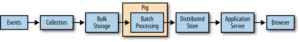
Figure 3-4. Processing data with Pig

Installing Pig

At the time of writing, Pig 0.11 is the latest version. Check here to see if there is a newer version, and if so, use it instead: http://pig.apache.org/releases.html.

To install Pig on your local machine, follow the Getting Started directions at http://pig.apache.org/docs/r0.11.0/start.html.

cd /me

wget http://apache.osuosl.org/pig/pig-0.11.1/pig-0.11.1.tar.gz

tar -xvzf pig-0.11.1.tar.gz

cd pig-0.11.1

ant

cd contrib/piggybank/java

ant

echo 'export PATH=$PATH:/me/pig-0.11.1/bin' >> ~/.bash_profile

source ~/.bash_profile

Now test Pig on the emails from your inbox we stored as avros. Run Pig in local mode (instead of Hadoop mode) via -x local and put logfiles in /tmp via -l /tmp to keep from cluttering your workspace.

cd pig; pig -l /tmp -x local -v -w sent_counts.pig

Our Pig script, ch03/pig/sent_counts.pig, flows our data through filters to clean it, and then projects, groups, and counts it to determine sent counts (Example 3-5).

Example 3-5. Processing data with Pig

/* Set Home Directory - where we install software */

%default HOME `echo \$HOME/Software/`

DEFINE AvroStorage org.apache.pig.piggybank.storage.avro.AvroStorage();

rmf /tmp/sent_counts.txt

/* Load the emails in avro format (edit the path to match where you saved them)

using the AvroStorage UDF from Piggybank */

messages = LOAD '/me/Data/test_mbox' USING AvroStorage();

/* Filter nulls, they won't help */

messages = FILTER messages BY (from IS NOT NULL) AND (tos IS NOT NULL);

/* Emails can be 'to' more than one person. FLATTEN() will project our from with

each 'to' that exists. */addresses = FOREACH messages GENERATE from.address AS

from, FLATTEN(tos.(address)) AS to;

/* Lowercase the email addresses, so we don't count MiXed case of the same address

as multiple addresses */lowers = FOREACH addresses GENERATE LOWER(from) AS from,

LOWER(to) AS to;

/* GROUP BY each from/to pair into a bag (array), then count the bag's contents

($1 means the 2nd field) to get a total.

Same as SQL: SELECT from, to, COUNT(*) FROM lowers GROUP BY (from, to);

Note: COUNT_STAR differs from COUNT in that it counts nulls. */

by_from_to = GROUP lowers BY (from, to);

sent_counts = FOREACH by_from_to GENERATE FLATTEN(group) AS (from, to),

COUNT_STAR(lowers) AS total;

/* Sort the data, highest sent count first */

sent_counts = ORDER sent_counts BY total DESC;

STORE sent_counts INTO '/tmp/sent_counts.txt';

Since we stored without specifying a storage function, Pig uses PigStorage. By default, PigStorage produces tab-separated values. We can simply cat the file, or open it in Excel (as shown in Figure 3-5).

cat /tmp/sent_counts.txt/part-*

erictranslates@gmail.com d3-js@googlegroups.com 1

info@meetup.com russell.jurney@gmail.com 1

jira@apache.org pig-dev@hadoop.apache.org 1

desert_rose_170@hotmail.com user@hbase.apache.org 1

fnickels@gmail.com d3-js@googlegroups.com 1

l.garulli@gmail.com gremlin-users@googlegroups.com 1

punk.kish@gmail.com d3-js@googlegroups.com 1

lists@ruby-forum.com user@jruby.codehaus.org 1

rdm@cfcl.com ruby-99@meetup.com 1

sampd@stumbleupon.com user@pig.apache.org 1

sampd@stumbleupon.com user@hive.apache.org 1

kate.jurney@gmail.com russell.jurney@gmail.com 2

bob@novus.com d3-js@googlegroups.com 2

dalia.mohsobhy@hotmail.com user@hbase.apache.org 2

hugh.lomas@lodestarbpm.com d3-js@googlegroups.com 2

update+mkd57whm@facebookmail.com russell.jurney@gmail.com 2

notification+mkd57whm@facebookmail.com 138456936208061@groups.facebook.com 3

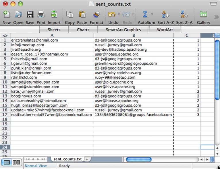
Pig output in Microsoft Excel spreadsheet

Figure 3-5. Pig output in Excel

You can see how the data flows in Figure 3-6. Each line of a Pig Latin script specifies some transformation on the data, and these transformations are executed stepwise as data flows through the script.

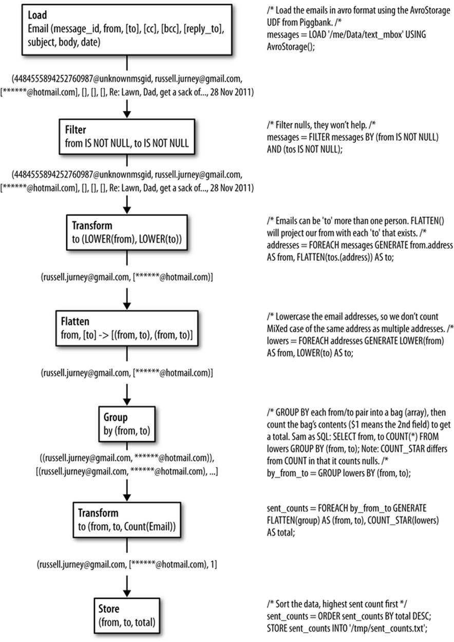
Figure 3-6. Dataflow through a Pig Latin script

Publishing Data with MongoDB

To feed our data to a web application, we need to publish it in some kind of database. While many choices are appropriate, we’ll use MongoDB for its ease of use, document orientation, and excellent Hadoop and Pig integration (Figure 3-7). With MongoDB and Pig, we can define any arbitrary schema in Pig, and mongo-hadoop will create a corresponding schema in MongoDB. There is no overhead in managing schemas as we derive new relations—we simply manipulate our data into publishable form in Pig. That’s agile!

Publishing Data

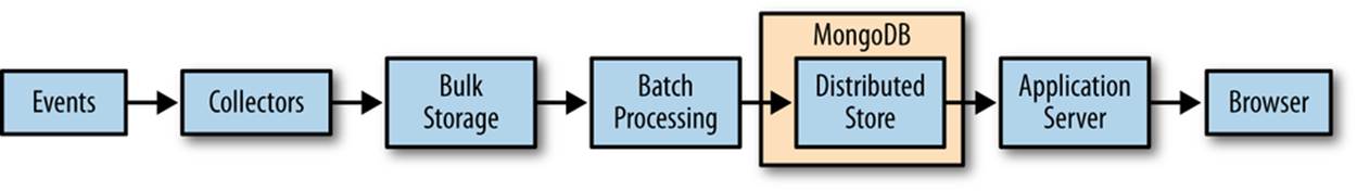
Figure 3-7. Publishing data to MongoDB

Installing MongoDB

Excellent instructions for installing MongoDB are available at http://www.mongodb.org/display/DOCS/Quickstart. An excellent tutorial is available here: http://www.mongodb.org/display/DOCS/Tutorial. I recommend completing these brief tutorials before moving on.

Download MongoDB for your operating system at http://www.mongodb.org/downloads.

cd /me

wget http://fastdl.mongodb.org/osx/mongodb-osx-x86_64-2.0.2.tgz

tar -xvzf mongodb-osx-x86_64-2.0.2.tgz

sudo mkdir -p /data/db/

sudo chown `id -u` /data/db

Now start the MongoDB server:

cd /me/mongodb-osx-x86_64-2.0.2

bin/mongodb 2>&1 &

Now open the mongo shell, and get help:

bin/mongo

> help

Finally, create our collection and insert and query a record:

> use agile_data

> e = {from: 'russell.jurney@gmail.com', to: 'bumper1700@hotmail.com',

subject: 'Grass seed', body: 'Put grass on the lawn...'}

> db.email.save(e)

> db.email.find()

{ "_id" : ObjectId("4f21c5f7c6ef8a98a43d921b"), "from" :

"russell.jurney@gmail.com",

"to" : "bumper1700@hotmail.com", "subject" : "Grass seed",

"body" : "Put grass on the lawn..." }

We’re cooking with Mongo! We’ll revisit this operation later.

Installing MongoDB’s Java Driver

MongoDB’s Java driver is available at https://github.com/mongodb/mongo-java-driver/downloads. At the time of writing, the 2.10.1 version is the latest stable build: https://github.com/downloads/mongodb/mongo-java-driver/mongo-2.10.1.jar.

wget https://github.com/downloads/mongodb/mongo-java-driver/mongo-2.10.1.jar

mv mongo-2.10.1.jar /me/mongo-hadoop/

Installing mongo-hadoop

Once we have the Java driver to MongoDB, we’re ready to integrate with Hadoop. MongoDB’s Hadoop integration is available at https://github.com/mongodb/mongo-hadoop and can be downloaded at https://github.com/mongodb/mongo-hadoop/tarball/master as a tar/gzip file.

cd /me

git clone git@github.com:rjurney/mongo-hadoop.git

cd mongo-hadoop

sbt package

Pushing Data to MongoDB from Pig

Pushing data to MongoDB from Pig is easy.

First we’ll run ch03/pig/mongo.pig to store the sent counts we computed to MongoDB, as shown in Example 3-6.

Example 3-6. Pig to MongoDB (ch03/pig/mongo.pig)

set mapred.map.tasks.speculative.execution false

set mapred.reduce.tasks.speculative.execution false

sent_counts = LOAD '/tmp/sent_counts.txt' AS (from:chararray, to:chararray, total:long);

STORE sent_counts INTO 'mongodb://localhost/agile_data.sent_counts' USING

com.mongodb.hadoop.pig.MongoStorage();

Now we’ll query our data in Mongo!

use agile_data

> db.sent_counts.find()

{ "from" : "erictranslates@gmail.com", "to" : "d3-js@googlegroups.com",

"total" : 1 }

{ "from" : "info@meetup.com", "to" : "russell.jurney@gmail.com",

"total" : 1 }

{ "from" : "jira@apache.org", "to" : "pig-dev@hadoop.apache.org",

"total" : 1 }

{ "from" : "desert_rose_170@hotmail.com", "to" : "user@hbase.apache.org",

"total" : 1 }

{ "from" : "fnickels@gmail.com", "to" : "d3-js@googlegroups.com",

"total" : 1 }

{ "from" : "l.garulli@gmail.com", "to" : "gremlin-users@googlegroups.com",

"total" : 1 }

{ "from" : "punk.kish@gmail.com", "to" : "d3-js@googlegroups.com",

"total" : 1 }

{ "from" : "lists@ruby-forum.com", "to" : "user@jruby.codehaus.org",

"total" : 1 }

{ "from" : "rdm@cfcl.com", "to" : "ruby-99@meetup.com", "total" : 1 }

{ "from" : "sampd@stumbleupon.com", "to" : "user@pig.apache.org",

"total" : 1 }

{ "from" : "sampd@stumbleupon.com", "to" : "user@hive.apache.org",

"total" : 1 }

{ "from" : "kate.jurney@gmail.com", "to" : "russell.jurney@gmail.com",

"total" : 2 }

{ "from" : "bob@novus.com", "to" : "d3-js@googlegroups.com",

"total" : 2 }

{ "from" : "dalia.mohsobhy@hotmail.com", "to" : "user@hbase.apache.org",

"total" : 2 }

{ "from" : "hugh.lomas@lodestarbpm.com", "to" : "d3-js@googlegroups.com",

"total" : 2 }

{ "from" : "update+mkd57whm@facebookmail.com", "to" : "russell.jurney@gmail.com",

"total" : 2 }

{ "from" : "notification+mkd57whm@facebookmail.com", "to" :

"138456936208061@groups.facebook.com", "total" : 3 }

> db.sent_counts.find({from: 'kate.jurney@gmail.com', to:

'russell.jurney@gmail.com'})

{ "from" : "kate.jurney@gmail.com", "to" : "russell.jurney@gmail.com",

"total" : 2 }

Congratulations, you’ve published Agile Big Data! Note how easy that was: once we had our data prepared, it is a one-liner to publish it with Mongo! There is no schema overhead, which is what we need for how we work. We don’t know the schema until we’re ready to store, and when we do, there is little use in specifying it externally to our Pig code. This is but one part of the stack, but this property helps us work rapidly and enables agility.

SPECULATIVE EXECUTION AND HADOOP INTEGRATION

We haven’t set any indexes in MongoDB, so it is possible for copies of entries to be written. To avoid this, we must turn off speculative execution in our Pig script.

set mapred.map.tasks.speculative.execution false

Hadoop uses a feature called speculative execution to fight skew, the bane of concurrent systems. Skew is when one part of the data, assigned to some part of the system for processing, takes much longer than the rest of the data. Perhaps there are 10,000 entries for all keys in your data, but one has 1,000,000. That key can end up taking much longer to process than the others. To combat this, Hadoop runs a race—multiple mappers or reducers will process the lagging chunk of data. The first one wins!

This is fine when writing to the Hadoop filesystem, but this is less so when writing to a database without primary keys that will happily accept duplicates. So we turn this feature off in Example 3-6, via set mapred.map.tasks.speculative.execution false.

Searching Data with ElasticSearch

ElasticSearch is emerging as “Hadoop for search,” in that it provides a robust, easy-to-use search solution that lowers the barrier of entry to individuals wanting to search their data, large or small. ElasticSearch has a simple RESTful JSON interface, so we can use it from the command line or from any language. We’ll be using ElasticSearch to search our data, to make it easy to find the records we’ll be working so hard to create.

Installation

Excellent tutorials on ElasticSearch are available at http://www.elasticsearchtutorial.com/elasticsearch-in-5-minutes.html and https://github.com/elasticsearch/elasticsearch#getting-started.

ElasticSearch is available for download at http://www.elasticsearch.org/download/.

wget https://github.com/downloads/elasticsearch/elasticsearch/

elasticsearch-0.20.2.tar.gz

tar -xvzf elasticsearch-0.20.2.tar.gz

cd elasticsearch-0.20.2

mkdir plugins

bin/elasticsearch -f

That’s it! Our local search engine is up and running!

ElasticSearch and Pig with Wonderdog

Infochimps’ Wonderdog provides integration between Hadoop, Pig, and ElasticSearch. With Wonderdog, we can load and store data from Pig to and from our search engine. This is extremely powerful, because it lets us plug a search engine into the end of our data pipelines.

Installing Wonderdog

You can download Wonderdog here: https://github.com/infochimps-labs/wonderdog.

git clone https://github.com/infochimps-labs/wonderdog.git

mvn install

Wonderdog and Pig

To use Wonderdog with Pig, load the required jars and run ch03/pig/elasticsearch.pig.

/* Avro uses json-simple, and is in piggybank until Pig 0.12, where AvroStorage

and TrevniStorage are builtins */

DEFINE AvroStorage org.apache.pig.piggybank.storage.avro.AvroStorage();

/* Elasticsearch's own jars */

/* Register wonderdog - elasticsearch integration */

/* Remove the old json */

rmf /tmp/sent_count_json

/* Nuke the elasticsearch sent_counts index, as we are about to replace it. */

sh curl -XDELETE 'http://localhost:9200/inbox/sent_counts'

/* Load Avros, and store as JSON */

sent_counts = LOAD '/tmp/sent_counts.txt' AS (from:chararray, to:chararray,

total:long);

STORE sent_counts INTO '/tmp/sent_count_json' USING JsonStorage();

/* Now load the JSON as a single chararray field, and index it into ElasticSearch

with Wonderdog from InfoChimps */

sent_count_json = LOAD '/tmp/sent_count_json' AS (sent_counts:chararray);

STORE sent_count_json INTO 'es://inbox/sentcounts?json=true&size=1000' USING

com.infochimps.elasticsearch.pig.ElasticSearchStorage(

'$HOME/elasticsearch-0.20.2/config/elasticsearch.yml',

'$HOME/elasticsearch-0.20.2/plugins');

/* Search for Hadoop to make sure we get a hit in our sent_count index */

sh curl -XGET 'http://localhost:9200/inbox/sentcounts/_search?q=russ&pretty=

true&size=1'

Searching our data

Now, searching our data is easy, using curl:

curl -XGET 'http://localhost:9200/sent_counts/sent_counts/_search?q=

russell&pretty=true'

{

"took" : 4,

"timed_out" : false,

"_shards" : {

"total" : 5,

"successful" : 5,

"failed" : 0

"hits" : {

"total" : 13,

"max_score" : 1.2463257,

"hits" : [ {

"_index" : "inbox",

"_type" : "sentcounts",

"_id" : "PmiMqM51SUi3L4-Xr9iDTw",

"_score" : 1.2463257, "_source" : {"to":"russell@getnotion.com","total":1,

"from":"josh@getnotion.com"}

}, {

"_index" : "inbox",

"_type" : "sentcounts",

"_id" : "iog-R1OoRYO32oZX-W1DUw",

"_score" : 1.2463257, "_source" : {"to":"russell@getnotion.com","total":7,"

from":"mko@getnotion.com"}

}, {

"_index" : "inbox",

"_type" : "sentcounts",

"_id" : "Y1VA0MX8TOW35sPuw3ZEtw",

"_score" : 1.2441664, "_source" : {"to":"russell@getnotion.com","total":1,

"from":"getnotion@jiveon.com"}

} ]

}

Clients for ElasticSearch for many languages are available at http://www.elasticsearch.org/guide/appendix/clients.html.

Python and ElasticSearch with pyelasticsearch

For Python, pyelasticsearch is a good choice. To make it work, we’ll first need to install the Python Requests library.

Using pyelasticsearch is easy: run ch03/pig/elasticsearch.pig.

import pyelasticsearch

elastic = pyelasticsearch.ElasticSearch('http://localhost:9200/inbox')

results = elastic.search("hadoop", index="sentcounts")

print results['hits']['hits'][0:3]

[

{

u'_score': 1.0898509,

u'_type': u'sentcounts',

u'_id': u'FFGklMbtTdehUxwezlLS-g',

u'_source': {

u'to': u'hadoop-studio-users@lists.sourceforge.net',

u'total': 196,

u'from': u'hadoop-studio-users-request@lists.sourceforge.net'

u'_index': u'inbox'

{

u'_score': 1.084789,

u'_type': u'sentcounts',

u'_id': u'rjxnV1zST62XoP6IQV25SA',

u'_source': {

u'to': u'user@hadoop.apache.org',

u'total': 2,

u'from': u'hadoop@gmx.com'

u'_index': u'inbox'

{

u'_score': 1.084789,

u'_type': u'sentcounts',

u'_id': u'dlIdbCPjRcSOLiBZkshIkA',

u'_source': {

u'to': u'hadoop@gmx.com',

u'total': 1,

u'from': u'billgraham@gmail.com'

u'_index': u'inbox'

}

]

Reflecting on our Workflow

Compared to querying MySQL or MongoDB directly, this workflow might seem hard. Notice, however, that our stack has been optimized for time-consuming and thoughtful data processing, with occasional publishing. Also, this way we won’t hit a wall when our real-time queries don’t scale anymore as they becoming increasingly complex.

Once our application is plumbed efficiently, the team can work together efficiently, but not before. The stack is the foundation of our agility.

Lightweight Web Applications

The next step is turning our published data into an interactive application. As shown in Figure 3-8, we’ll use lightweight web frameworks to do that.

Data Applications

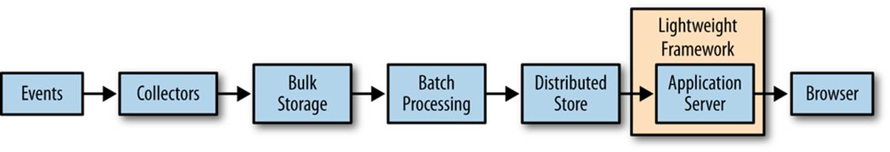
Figure 3-8. To the Web with Python and Flask

We choose lightweight web frameworks because they are simple and fast to work with. Unlike CRUD applications, mined data is the star of the show here. We use read-only databases and simple application frameworks because that fits with the applications we build and how we offer value.

Given the following examples in Python/Flask, you can easily implement a solution in Sinatra, Rails, Django, Node.js, or your favorite language and web framework.

Python and Flask

According to the Bottle Documentation, “Flask is a fast, simple, and lightweight WSGI micro web framework for Python.”

Excellent instructions for using Flask are available at http://flask.pocoo.org/.

Flask Echo ch03/python/flask_echo.py

Run our echo Flask app, ch03/python/flask_echo.py.

fromflaskimport Flask

app = Flask(__name__)

@app.route("/<input>")

def hello(input):

return input

if __name__ == "__main__":

app.run(debug=True)

$ curl http://localhost:5000/hello%20world!

hello world!

Python and Mongo with pymongo

Pymongo presents a simple interface for MongoDB in Python. To test it out, run ch03/python/flask_echo.py.

importpymongo

importjson

conn = pymongo.Connection() # defaults to localhost

db = conn.agile_data

results = db['sent_counts'].find()

for i inrange(0, results.count()): # Loop and print all results

print results[i]

The output is like so:

{u'total': 22994L, u'to': u'pig-dev@hadoop.apache.org', u'_id': ObjectId

('50ea5e0a30040697fb0f0710'), u'from': u'jira@apache.org'}

{u'total': 3313L, u'to': u'russell.jurney@gmail.com', u'_id': ObjectId

('50ea5e0a30040697fb0f0711'), u'from': u'twitter-dm-russell.jurney=

gmail.com@postmaster.twitter.com'}

{u'total': 2406L, u'to': u'russell.jurney@gmail.com', u'_id': ObjectId

('50ea5e0a30040697fb0f0712'), u'from': u'notification+mkd57whm@facebookmail.com'}

{u'total': 2353L, u'to': u'russell.jurney@gmail.com', u'_id': ObjectId

('50ea5e0a30040697fb0f0713'), u'from': u'twitter-follow-russell.jurney=

gmail.com@postmaster.twitter.com'}

Displaying sent_counts in Flask

Now we use pymongo with Flask to display the sent_counts we stored in Mongo using Pig and MongoStorage. Run ch03/python/flask_mongo.py.

fromflaskimport Flask

importpymongo

importjson

# Set up Flask

app = Flask(__name__)

# Set up Mongo

conn = pymongo.Connection() # defaults to localhost

db = conn.agile_data

sent_counts = db['sent_counts']

# Fetch from/to totals, given a pair of email addresses

@app.route("/sent_counts/<from_address>/<to_address>")

def sent_count(from_address, to_address):

sent_count = sent_counts.find_one( {'from': from_address, 'to': to_address} )

return json.dumps( {'from': sent_count['from'], 'to': sent_count['to'], 'total'

: sent_count['total']} )

if __name__ == "__main__":

app.run(debug=True)

Now visit a URL you know will contain records from your own inbox (for me, this is http://localhost:5000/sent_counts/russell.jurney@gmail.com/*******@gmail.com) and you will see:

{"ego1":"russell.jurney@gmail.com","ego2":"*******@gmail.com","total":8}

And we’re done! (See Figure 3-9).

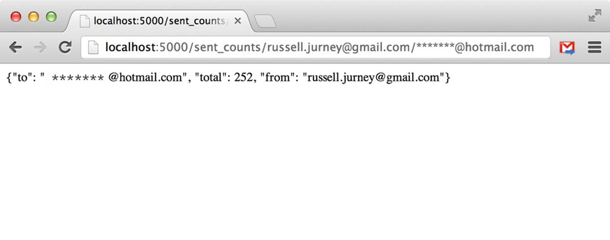
{"ego1”:"k@123.org”,"ego2”:"common-user@hadoop.apache.org”,"total”:8}

Figure 3-9. Undecorated data on the Web

Congratulations! You’ve published data on the Web. Now let’s make it presentable.

Presenting Our Data

Design and presentation impact the value of your work. In fact, one way to think of Agile Big Data is as data design. The output of our data models matches our views, and in that sense design and data processing are not distinct. Instead, they are part of the same collaborative activity: data design. With that in mind, it is best that we start out with a solid, clean design for our data and work from there (see Figure 3-10).

Presentation in the user’s browser

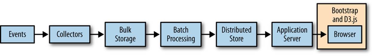
Figure 3-10. Presenting our data with Bootstrap and D3.js and nvd3.js

Installing Bootstrap

According to the Bootstrap Project:

Bootstrap is Twitter’s toolkit for kickstarting CSS for websites, apps, and more. It includes base CSS styles for typography, forms, buttons, tables, grids, navigation, alerts, and more.

Bootstrap is available at http://twitter.github.com/bootstrap/assets/bootstrap.zip. To install, place it with the static files of your application and load it in an HTML template.

wget http://twitter.github.com/bootstrap/assets/bootstrap.zip

unzip bootstrap.zip

We’ve already installed Bootstrap at ch03/web/static/bootstrap.

To invoke Bootstrap, simply reference it as CSS from within your HTML page—for example, from ch03/web/templates/table.html.

Booting Boostrap

It takes only a little editing of an example to arrive at a home page for our project, as shown in Figure 3-11.

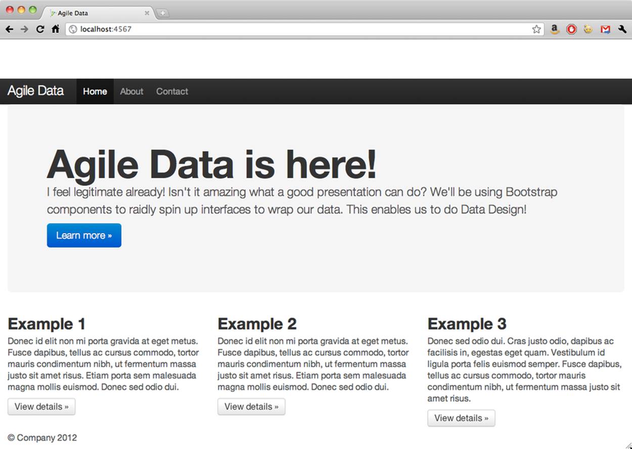
Agile Big Data Homepage, with the text: I feel legitimate already (because this web page has pretty CSS)! Isn’t it amazing what a good presentation can do? We’ll be using Bootstrap components to rapidly spin up interfaces to wrap our data. This enables us to do Data Design!

Figure 3-11. Bootstrap 2.0 hero example

Let’s try wrapping a previous example in a table, styled with Bootstrap.

That’s right: tables for tabular data! Bootstrap lets us use them without shame. Now we’ll update our controller to stash our data, and create a simple template to print a table.

In index.py:

fromflaskimport Flask, render_template

importpymongo

importjson

importre

# Set up Flask

app = Flask(__name__)

# Set up Mongo

conn = pymongo.Connection() # defaults to localhost

db = conn.agile_data

# Fetch from/to totals and list them

@app.route("/sent_counts")

def sent_counts():

sent_counts = db['sent_counts'].find()

results = {}

results['keys'] = 'from', 'to', 'total'

results['values'] = [[s['from'], s['to'], s['total']]

for s insent_counts if re.search('apache', s['from']) or

re.search('apache', s['to'])]

results['values'] = results['values'][0:17]

return render_template('table.html', results=results)

if __name__ == "__main__":

app.run(debug=True)

And in our template, table.html:

<!DOCTYPE html>

<head>

<title>Agile Big Data - Inbox Explorer</title>

<!-- Derived from example at http://twitter.github.com/bootstrap/

examples/sticky-footer.html -->

/* Sticky footer styles

-------------------------------------------------- */

html,

body {

height: 100%;

/* The html and body elements cannot have any padding or margin. */

}

/* Wrapper for page content to push down footer */

#wrap {

min-height: 100%;

height: auto !important;

height: 100%;

/* Negative indent footer by it's height */

margin: 0 auto -60px;

}

/* Set the fixed height of the footer here */

#push,

#footer {

height: 60px;

}

#footer {

background-color: #f5f5f5;

}

/* Lastly, apply responsive CSS fixes as necessary */

@media (max-width: 767px) {

#footer {

margin-left: -20px;

margin-right: -20px;

padding-left: 20px;

padding-right: 20px;

}

/* Custom page CSS

-------------------------------------------------- */

/* Not required for template or sticky footer method. */

.container {

width: auto;

max-width: 1000px;

}

.container .credit {

margin: 20px 0;

}

.container[role="main"] {

padding-bottom: 60px;

}

#footer {

position: fixed;

bottom: 0;

left: 0;

right: 0;

}

.lead { margin-top: -15px; }

</style>

<!--[if lt IE 9]>

<![endif]-->

</head>

<body>

<h1>Analytic Inbox</h1>

</div>

<p class="lead">Email Sent Counts</p>

<thead>

{% for key in results['keys'] -%}

{% endfor -%}

</thead>

<tbody>

{% for row in results['values'] -%}

<tr>

{% for value in row -%}

<td>{{value}}</td>

{% endfor -%}

</tr>

{% endfor -%}

</tbody>

</table>

</div>

</div>

<!-- <p class="muted credit">Example courtesy <a href="http://martinbean.

co.uk">Martin Bean</a> and <a href="http://ryanfait.com/sticky-

footer/">Ryan Fait</a>.</p> -->

<p class="muted credit"><a href="http://shop.oreilly.com/product/

0636920025054.do">Agile Big Data</a> by <a href="http://

www.linkedin.com/in/russelljurney">Russell Jurney</a>, 2013

</div>

<!-- Le javascript

================================================== -->

</body>

</html>

The result, shown in Figure 3-12, is human-readable data with very little trouble!

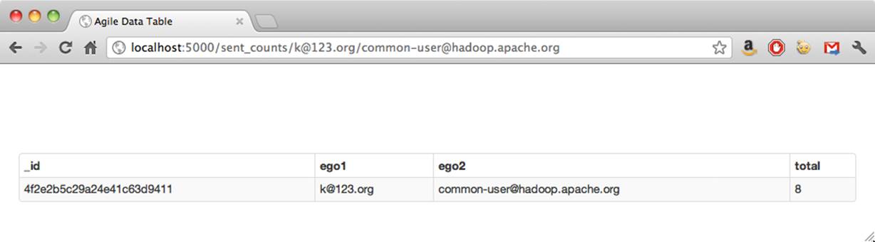
Application logic moves between batch processing all the way to the browser in Agile Big Data, as needed.

Figure 3-12. Simple data in a Bootstrap-styled table

NOTE

In practice, we may use client-side templating languages like moustache. For clarity’s sake, we use Jinja2 templates in this book.

Visualizing Data with D3.js and nvd3.js

D3.js enables data-driven documents. According to its creator, Mike Bostock:

d3 is not a traditional visualization framework. Rather than provide a monolithic system with all the features anyone may ever need, d3 solves only the crux of the problem: efficient manipulation of documents based on data. This gives d3 extraordinary flexibility, exposing the full capabilities of underlying technologies such as CSS3, HTML5, and SVG.

We’ll be using D3.js to create charts in our application. Like Bootstrap, it is already installed in /static.

wget d3js.org/d3.v3.zip

We’ll be making charts with D3.js and nvd3.js later on. For now, take a look at the examples directory to see what is possible with D3.js: https://github.com/mbostock/d3/wiki/Gallery and http://nvd3.org/ghpages/examples.html.

Conclusion

We’ve created a very simple app with a single, very simple feature. This is a great starting point, but so what?

What’s important about the application isn’t what it does, but rather that it’s a pipeline where it’s easy to modify every stage. This is a pipeline that will scale without our worrying about optimization at each step, and where optimization becomes a function of cost in terms of resource efficiency, but not in terms of the cost of reengineering.

As we’ll see in the next chapter, because we’ve created an arbitrarily scalable pipeline where every stage is easily modifiable, it is possible to return to agility. We won’t quickly hit a wall as soon as we need to switch from a relational database to something else that “scales better,” and we aren’t subjecting ourselves to the limitations imposed by tools designed for other tasks like online transaction processing (Figure 3-13).

We now have total freedom to use best-of-breed tools within this framework to solve hard problems and produce value. We can choose any language, any framework, and any library and glue it together to get things built.

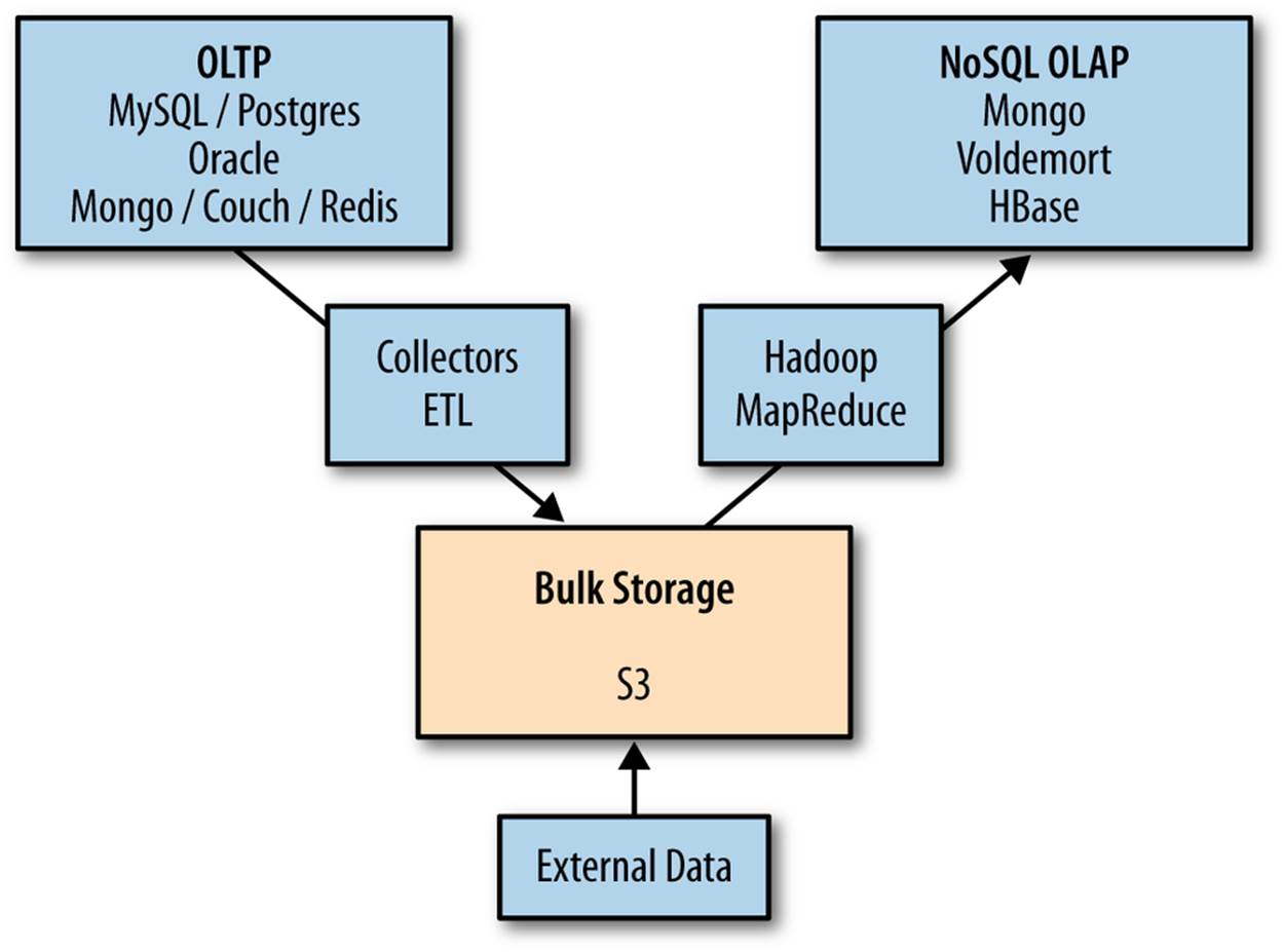
Figure 3-13. Online Transaction Processing (OLTP) and NoSQL OnLine Analytic Processing (OLAP)