F# Deep Dives (2015)

Part 2. Developing analytical components

When talking about F# from a business perspective in chapter 1, we mostly focused on the development of analytical components. These are the components that underlie the business value of an application. Think about financial models, artificial intelligence in games, recommendation engines in retail applications, and data analysis and visualization components.

As you saw in chapter 1, choosing F# for developing analytical components will solve existing problems for your business, including taming complexity, guaranteeing correctness and performance of solutions, and making it easier and faster to turn an application from an idea and a prototype into a deployed system.

The chapters in this part of the book demonstrate many of these benefits using three interesting practical problems. In chapter 4, Chao-Jen Chen will explore the implementation of financial models in F#. Even if you’re not familiar with the models discussed in the chapter, you can see that F# makes it easy to turn the mathematics behind the models into code that is correct and efficient. In chapter 5, Evelina Gabasova demonstrates how to analyze and visualize social network data. Explaining why this is important would be a waste of space—your systems can get enormous value from your understanding of social networks. It’s amazing how much you can achieve in a single chapter! Finally, Keith Battocchi demonstrates a recent F# feature called type providers. Chapter 6 shows how you can integrate external data into F#, making it extremely easy for other developers on the team to access rich data sources.

In general, if you’re interested in implementing calculations, data transformations, processing of business rules, or any functionality with important business logic, choosing F# is the right option. The chapters in this part of the book only scratch the surface of what you can do, but you can find a number of other experience reports on the F# Software Foundation website at www.fsharp.org.

Chapter 4. Numerical computing in the financial domain

Chao-Jen Chen

The modern finance industry can’t operate without numerical computing. Financial institutions, such as investment banks, hedge funds, commercial banks, and even central banks, heavily use various numerical methods for derivatives pricing, hedging, and risk management. Usually the production systems of those numerical methods are implemented in general-purpose object-oriented languages like C++, C#, and Java. But there’s a steady, emerging trend in the industry: financial institutions are increasingly adopting functional languages, including F#, when implementing their new derivatives-pricing or risk-control systems. One of the reasons this is happening is that a functional language like F# is relatively expressive in turning mathematical equations into code. Moreover, F# has strong support for high-performance computing techniques, such as graphics processing unit (GPU) computing and parallelization. As such, F# enables programmers and quantitative analysts to spend less time coding and at the same time avoid compromising performance.

Among the numerical methods widely used in the finance industry, we’ve chosen Monte Carlo simulation and its applications to derivatives pricing as our main topic. This chapter serves as an example of how F# is a good fit for implementing analytical components like a derivatives pricing engine, as mentioned in chapter 1. In this chapter, you’ll see how F#’s functional features can help you write concise code for Monte Carlo simulation and, more important, make the code generic so that you can apply the same simulation code to pricing various types of derivatives. If you were to do the same in a typical object-oriented language, you’d have to implement different types of derivatives as classes and have them inherit a common abstract class or implement the same interface. Thanks to higher-order functions and function currying in F#, you don’t have to construct the cumbersome inheritance hierarchy (although you could still choose to do that in F# because F# also supports the object-oriented style of polymorphism).

Introducing financial derivatives and underlying assets

A financial derivative is a contract that usually involves two parties, buyer and seller, and is defined in terms of some underlying asset that already exists on the market. The payoff of a financial derivative is contingent on the market price of its underlying asset at some time point in the future, such as the agreed expiry time of a contract. Many different types of financial derivatives are traded on the market. Our discussion here is limited to a tiny slice of the derivatives world. The types of financial derivatives we’ll be looking at in this chapter are all European style—that is, each derivative contract has only one payoff at the expiration date and has no early-exercise feature.

Before we describe the derivatives we’ll be looking at, let’s talk about underlying assets. Although there are all kinds of underlying assets, such as equities, bonds, crude oil, gold, and even live stocks, this chapter focuses only on stocks as underlying assets. More precisely, we’ll look at only non-dividend-paying stocks. One famous example of non-dividend-paying stocks is Warren Buffett’s Berkshire Hathaway Holding, which never pays any dividends.

Non-dividend-paying stocks

Why do we assume that underlying assets have to be non-dividend-paying? Because we need more complicated mathematical treatments in order to model dividend-paying behaviors, which is too much to cover here. But as far as derivatives pricing is concerned, the scope of non-dividend-paying stocks is perhaps broader than your imagination. As long as the underlying stock of the derivative contract you’re considering doesn’t pay out any dividend during the period from today to the expiry of the derivative, the stock can be viewed as a non-dividend-paying stock when you price the derivative contract. Derivatives with stocks as underlying assets are usually called stock options or equity options.

European call options

Let’s assume that, for a non-dividend-paying stock _S, S_t denotes its share price at time t. Then, a European call option with strike K and expiry T on stock S pays max(S_T – K,0) to the holder of the call option at time T. In other words, the call option pays (S_T – K) to the option holder if S_T (the share price at the expiry of the call option) exceeds _K, and it pays nothing otherwise. For convenience, we’ve defined a shorthand notation for max(S_T – K,0). Given any real number _r, (r)⁺ = max(r,0), which is called a positive part function. So the European call payoff max(S_T – K,0) can be shortened to (S_T – K)⁺.

Before we jump into derivatives pricing, let’s review some fundamental probability concepts that you’ll need in this chapter.

Using probability functions of Math.NET

Probability theory underlies most pricing algorithms. We’ll explain all the important concepts as we go. In addition to probability, we also need to explain a bit about some F# settings you’ll need throughout the chapter. We’ll introduce Math.NET Numerics, an open source library, which you’ll use in Monte Carlo simulation.

Configuring F# Interactive

F# Interactive (FSI) is a great tool whereby you can execute F# code interactively, like other interactive numerical computing languages such as MathWorks’ MATLAB and Mathematica. If you want to test F# code, you type it in or send it to FSI and then immediately run it and get its results in FSI, which saves you from building an entire Visual Studio project just to do a small test. You’ll be using only FSI in this chapter, although you can also choose to create a new Visual Studio project.

Here’s another good thing about using FSI: it’s easy to profile your code—that is, to measure how much time your F# code takes for execution—because FSI comes with a built-in timing feature, which you’ll use later in this chapter. To enable FSI’s timing feature, type the #time command in FSI:

> #time;;

--> Timing now on

Another useful FSI setting is Floating Point Format, which controls how many decimal places FSI should print for a float. The default is 10, which is too many for this discussion. The following FSI command configures the printing:

> fsi.FloatingPointFormat <- "f5";;

val it : unit = ()

> 10.0/3.0;;

val it : float = 3.33333

As you can see, floating-point values are now printed with only five decimal places, which is enough for our purpose.

Downloading and setting up Math.NET Numerics

The Math.NET project (www.mathdotnet.com) is a set of open source libraries for different purposes, including numerical computing, signal processing, and computer algebra. Among those libraries, you’ll need only Math.NET Numerics, which you’ll use to generate random numbers and compute basic statistics. You can get Math.NET from http://numerics.mathdotnet.com or via the NuGet package MathNet.Numerics; the latest version as of this writing is v2.6.2. Assuming the library is installed in the Program Files folder, you can load it in FSI as follows:

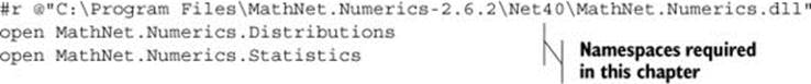
You’ll use the Normal class defined in the namespace MathNet.Numerics.Distributions and the extension method Variance() defined in the class MathNet.Numerics .Statistics.Statistics.

Random variables, expectation, and variance

The first mathematical thing you need to know about is the concept of random variables, because stock prices in the future are random as of today. Monte Carlo simulation itself is also a random variable.

Random variables

As you may know, there are two types of random variables: discrete and continuous. A discrete random variable is one that has a (finitely or infinitely) countable range, like the set of all positive integers. In contrast, a continuous random variable has an uncountable range, like all positive reals or all the reals between 0 and 1. As far as the Monte Carlo methods and stochastic processes you’ll use in this chapter are concerned, you need only continuous random variables.

A random variable X is a function that maps random events to real values. A value produced by X is called a sample drawn from random variable X. Due to randomness, every time you try to draw a sample from X, you get a different value. You can’t know for sure what value X will produce next until you’ve drawn the next sample from X. Although you can’t know beforehand what the next sample will be, you can study the probability for a particular range of values to be taken by X. This question can be answered by X’s probability density function f(x), which satisfies the following conditions:

f(x) ≥ 0, for all x

(if x could take on values ranging from –∞ to ∞)

A random variable X has quite a few characteristics, which can be defined in terms of its probability density function. The Monte Carlo simulation, the most important one, is expectation IE[X].

Expectation

IE[X] denotes the expectation of random variable X and is defined as follows:

IE[X] = ∫^∞X · f(X)dX

As you can see, the mathematical definition involves integration. Usually there are a few ways to interpret the definition. One common, straightforward interpretation is that the expectation of a random variable is the weighted average of all possible values that the random variable can produce. Another interpretation, which is more relevant to our study of Monte Carlo simulation, is that if you could draw infinitely many samples from X, IE[X] should equal the average of those samples. To a certain extent, Monte Carlo simulation computes the integral numerically.

In this chapter, you’ll use arrays to hold random samples. Why adopt arrays rather than other immutable data structures like lists or sequences? Because arrays are a few times faster than lists or sequences with respect to the operations you need here. Let’s take a quick look at computing the average of an array of samples. You’ll use the Array.average function provided by the F# Core Library:

> let x = [|1.0..10000000.0|];;

Real: 00:00:01.199, CPU: 00:00:01.216, GC gen0: 2, gen1: 2, gen2: 2

// the printout of x is not included as it is long and irrelevant.

> let avg1 = x |> Array.average;;

Real: 00:00:00.119, CPU: 00:00:00.124, GC gen0: 0, gen1: 0, gen2: 0

val avg1 : float = 5000000.50000

> let avg2 = x.Mean();;

Real: 00:00:00.244, CPU: 00:00:00.234, GC gen0: 0, gen1: 0, gen2: 0

val avg2 : float = 5000000.50000

In addition to the Array.average function, the example shows the extension method Mean() provided by MathNet.Numerics, which can also produce the sample average you want but is significantly slower than F#’s built-in Array.average function. That’s why you should use theArray.average function, but please note that the result of this comparison may vary from computer to computer. In other words, it’s possible that you’ll see the Mean() method run faster than the Array.average function.

Having described expectation, let’s proceed to another important characteristic of _X: variance, which plays a key role when later in this chapter we talk about how to measure and improve the accuracy of the Monte Carlo simulation.

Variance

Var(X) denotes the expectation of random variable X, which is defined as follows:

Var(X) = IE[(X – IE[X])²]

Var(X) is used to give you an idea of how a large number of samples from X are spread out: do they cluster in a small area, or do they spread across a wide range? People tend to dislike uncertainty; more often than not, you’d prefer a random variable with a lower variance. If you have to observe a random variable for whatever reason, you’ll usually want to see samples that cluster around expectation. This is exactly the case when it comes to Monte Carlo simulation. The smaller its variance is, the higher the simulation accuracy will be.

As for computation of variance, you’ll use the extension method Variance() from MathNet.Numerics. The following example shows how:

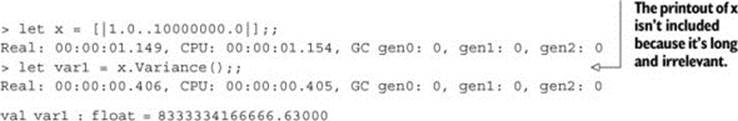
Now that you know how to observe the expectation and variance of a set of samples, let’s move on to producing those samples. You want them to follow a particular probability distribution.

Generating normal random samples

The only probability distribution you’ll use in this chapter is a normal distribution. You’ll generate normally distributed random samples and use those samples to simulate stock prices. Those simulated stock prices won’t be normally distributed—instead, based on the stochastic process employed here, they’ll be lognormally distributed. It’s easy to see that it doesn’t make sense to make stock prices normally distributed, because stock prices can’t go negative.

Normal distribution

Let N(u,σ²) denote a normal distribution with mean u and variance σ². If we say random variable X follows N(u,σ²), that means X has the following probability density function:

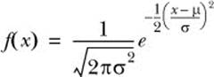
Perhaps you have already seen this expression because of the ubiquity of normal distributions, but we aren’t going to play with it algebraically. In this chapter we care only about how to draw samples from a random variable with the probability density function. The key point is that you use normal distribution to model the logarithmic return of the underlying asset.

Various algorithms are available for generating normal random samples. Fortunately, you don’t have to study and implement those algorithms yourself, because Math.NET has implemented a random number generator for normal distributions, which is sufficient for this study of Monte Carlo simulation. The following code snippet shows how to use the normal random number generator provided by Math.NET:

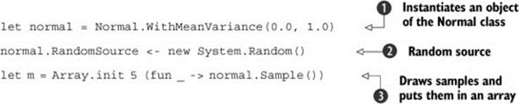
The code instantiates an object of the Normal class from the MathNet.Numerics.Distributions namespace . The object is named normal and represents a normal distribution with mean 0.0 and variance 1.0: N(0.0, 1.0). For this object to be able to generate normally distributed random samples, you have to give it a random source^[1]. The random source must be a direct or indirect instance of the System.Random class and is supposed to produce uniformly distributed random samples in the interval between 0.0 and 1.0. Math.NET provides a variety of alternatives for this purpose. But as far as this chapter is concerned, the System.Random class provided by the .NET Framework is sufficient. Having specified a random source, you invoke the normal.Sample() method^[2] to draw five samples from N(0.0, 1.0) and put them in an array named m .

¹ If you omit the second line, the Normal class will automatically use System.Random by default. But to make clear which uniform random number generators are being used, we chose to explicitly state it.

² The Sample method provided by Math.NET implements a popular algorithm for normal random number generation, the polar form of the Box-Muller transform.

Geometric Brownian motion and Monte Carlo estimates

This section begins our discussion of Monte Carlo simulation. The idea is that you create a model that generates a possible price path of the stock you’re interested in. For each generated price path of the stock, you can compute the payout of the derivative contract you’re pricing. Then you run the model several times and average the simulated payouts to get a Monte Carlo estimate of the contract’s payoff.

To model stock price movement, you’ll use so-called geometric Brownian motion (GBM). We’ll describe and define the Monte Carlo estimate and apply it to pricing a European call, an up-and-out barrier call, and an Asian call. Along the way, we’ll also explain how to analyze the accuracy of a Monte Carlo estimate. And finally, we’ll introduce a widely adopted technique for improving accuracy.

Modeling stock prices using geometric Brownian motion

If you’re considering a particular option—say, a three-month European call option on a stock—the first step to price it is to model the dynamics of the stock during a certain time interval, [0,T], where 0 is the current time and T is the option’s expiry expressed in terms of years. In the case of a three-month option, T = 0.25 years . You then divide time interval [0,T] into N periods. Each of the periods has length Δt := T/N. For n = 0,1,2, ... ,N, let t_n := nΔt be the nth time point. As such, you can see that t₀ = 0 and t_N = T. Assuming today’s share price is known and denoted by S_t0, simulating a price path means that you need to somehow simulate the following prices: S_t1, S_t2, S_t3, ..., S_tN.

To generate these prices, you have to choose a stochastic process to model the price movements of the stock. Generally speaking, a stochastic process is a sequence of random variables indexed by time. Each of these random variables represents the state of the stochastic process at a particular point in time. In this case, the sequence of random variables is {S_t1, S_t2, S_t3, ..., S_tN}. A stochastic process can be specified by doing the following:

· Giving an initial start point, which is S_tn in this case

· Defining the dynamics of the stock price ΔS_tn = S_{tN – 1} – S_tn

The idea is to define how the price changes between two consecutive time points in a path. If you can somehow sample all the differentials, {ΔS_t0, ΔS_t1, ΔS_t2, ..., ΔS_{tN – 1}}, then you can generate a full path of share prices because you can use the generated differentials to infer all the share prices in the path.

To model stock prices, researchers and practitioners use many different types of stochastic processes. GBM is probably the most fundamental stochastic process for the purpose of derivatives pricing. In a GBM process, ΔS_t0 is defined by the following stochastic differential equation (SDE):

ΔS_t0 = rS_tnΔt + σS_tnΔW_tn.

From this expression, you can see that ΔS_tn is defined as a sum of two terms—a drift term (rS_tnΔt) and a diffusion term (σS_tnΔW_tn)—where

· r is the risk-free interest rate paid by a bank account.^[3]

³ Why must the coefficient of the drift term be the interest rate r times share price? In short, because you assume that there exists one (and only one) bank account in your model, which pays interest at rate r continuously in time, and you use the bank account as numéraire—that is, you measure the value of assets in terms of a bank account rather than in terms of dollars. We can’t explain the entire theory in detail here. If you’re interested in the theoretic details, a good book to consult is The Concepts and Practice of Mathematical Finance, 2nd edition, by Mark S. Joshi (Cambridge University Press, 2008).

· σ is the annualized volatility of the stock, which is usually estimated based on historical price data of the stock and may be adjusted by traders based on their view on the market. For example, if the annualized volatility of Apple stock is 25%, it means that statistically the Apple stock might go either up or down by 25% in one year’s time on average. In other words, the higher the volatility, the more volatile the stock price.

· ΔW_tn is the Brownian increment at time t_n. As far as our study of Monte Carlo simulation is concerned, you can view it as a sample drawn from a normal distribution with mean ₀ and variance Δt. This is designed to model the uncertainty of share-price movement.

Although the definition of ΔS_tn looks simple, it’s an important model that almost every textbook in mathematical finance begins with, because it captures the following realistic ideas:^[4]

⁴ But the GBM setting for ΔS_tn also has drawbacks. The most criticized one is probably the assumption of volatility σ being a constant, which is strongly inconsistent with empirical results. Quite a few models address this issue. If interested, you can look up local volatility models and stochastic volatility models. Those models can be viewed as extensions of the GBM model by allowing volatility to change in time or randomly. In particular, stochastic volatility models are the primary ones being used to price stock options in the industry.

· Changes in a stock’s price ought to be proportional to its current price level. For example, a $10 move is more likely at S_tn = 100 than at S_tn = 20.

· A stock’s price can’t go negative. If you can let Δt go infinitesimal, it can be proved that the prices modeled by a GBM process never go negative, as long as the initial price S_t0 is positive.

If the description of ΔS_tn makes sense to you, the next thing we’d like you to consider is that usually you don’t directly simulate ΔS_tn. Instead, you simulate log differential ΔlogS_tn, which is how the logarithm of the price evolves. You do that for a few reasons. Two of them are as follows:

· When you run a simulation, you can’t let Δt go infinitesimal, not only because time complexity of the simulation may be overwhelming as Δt gets smaller and smaller, but also because all the floating-point data types you typically use to represent Δt have limited precision. Therefore, if you directly implement the definition of ΔS_tn, your simulation might generate one or more negative share prices, which is definitely wrong.

· Simulating by ΔlogS_tn isn’t as sensitive to the choice of length Δt as directly simulating by ΔS_tn.

Given this GBM definition of ΔS_tn, log differential ΔlogS_tn can be deduced^[5] as follows:

⁵ This is the result of applying the famous Ito’s Rule to the logarithm function and the GBM definition of ΔS_tn.

This is the mathematical expression you’ll implement. Neither of the two terms contains S_tn, which is why simulating by ΔlogS_tn is more robust. Once you’ve sampled all the log differentials, {ΔlogS_t0, ΔlogS_t1, ΔlogS_t2, ..., ΔlogS_{tn – 1}}, you can recover any absolute price level S_tn using the following formula:

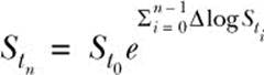
In other words, to compute S_tn you sum up all the log differentials from ΔlogS_t0 to ΔlogS_{tn –1}, exponentiate the sum, and multiply the exponentiated sum by S_t0. As you can see from the expression, if you simulate by ΔlogS_t0 rather than ΔS_tn, S_tn will always stay positive, regardless of how you choose Δt, because S_t0 is given positive and the exponential function always returns a positive value.

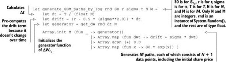
Now you’re ready to see how to write F# code to generate a GBM path by sampling ΔlogS_tn. Earlier you learned how to use the statistics functionality provided by Math.NET to generate random samples from a normal distribution with a particular mean and a particular variance. Let’s use that to come up with a function that can generate ΔW_tn. The function get_dW, shown in the following listing, is a higher-order function. get_dW returns a generator function, which generates N random samples from a normal distribution with mean ₀ and variance Δt.

Listing 1. Generating Brownian increments

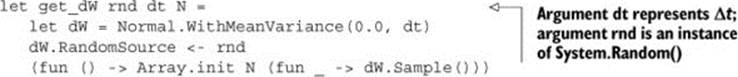
To generate a GBM path, you invoke the generator function returned by get_dW so as to generate N samples of ΔW_tn. Once you have the initial share price S_t0 and N samples of ΔW_tn, you can then infer a full stock-price path using the expression of S_tn in terms of ΔlogS_t1. If you repeat this procedure M times, you can then generate M different paths of stock prices, which is exactly what the following function does.

Listing 2. Generating GBM paths

Now you’re ready to generate some paths. Run the following in FSI:

let paths = generate_GBM_paths_by_log (new System.Random()) 50.0 0.01

0.2 0.25 200 3;;

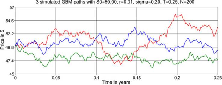
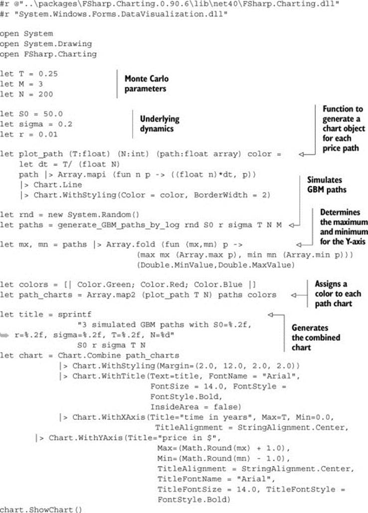
The array paths contains three different simulated stock-price paths. You can plot them using any charting software or API you like. The chart in figure 1 shows a sample of paths; we used the FSharp.Charting library to generate it, as shown in the accompanying sidebar. The chart you get will be different from this one due to randomness.

Figure 1. An example of using the generate_GBM_paths_by_log function to generate three paths of stock prices

Plotting stock price paths using FSharp.Charting

FSharp.Charting, an open source charting library for F#, provides a nice interface to the data-visualization charting controls available on Windows in .NET 4.x. You can download its source from GitHub or get the binary using NuGet. The following code shows how we generated figure 1:

Now that you’ve learned how to simulate paths of share prices of a stock, you can use these simulated paths to price a derivative—that is, to compute the price of the derivative at time 0.

Payoff function, discounted payoff, and Monte Carlo estimates

The types of derivatives we’re considering in this chapter are the ones that mature at time T, where T > 0, and pay only at time T a single cash flow. The amount of the cash flow at time T is contingent on how share prices evolve over the time interval _[0,T]—that is, the actual time-T payoff of the derivative is decided by a payoff function f of x and θ, where x is a path of share prices between time 0 and _T, and θ is a tuple of static parameters written in the derivative contract. Usually θ is called the contract parameters. The content of θ depends on the type of the derivative. If it’s a European call option with strike _K, then θ = (K). If it’s an up-and-out barrier option with strike K and barrier H, then θ = (K,H).

Time value of money

In this chapter, we assume that there exists a bank account paying continuously compound interest at an annualized rate _r, and that one dollar in the bank account today will be worth e^rT dollars by time T. As such, one dollar today and one dollar tomorrow aren’t the same thing. Before you can compare them, you have to either discount tomorrow’s one dollar back to today or compound today’s one dollar to tomorrow.

When you price a derivative whose payoff occurs at time T in the future, you need to discount it back to time 0 (today) by multiplying the payoff by a discounting factor e^–rT. If you don’t discount, you’ll misprice the derivative in the sense that you admit arbitrage.

Given static parameters θ and a particular price path _x, let Y := e^–rT · f(θ,x) denote the discounted payoff for the option represented by f(θ,x). Because the entire path x is random as of time 0, Y is also a random number as of time 0. If you simulate a price path _x, you can apply f to x in order to generate a sample of _Y. Therefore, although you may not know exactly the probability distribution of _Y, you do know how to draw a sample of it.

Let C denote the time-0 price of the derivative contract you’re considering. Using the fundamental theorem of asset pricing, you know that

C = IE[Y]

which is the expectation^[6] of Y. The problem is how to compute the expectation IE[Y]. If Y is a random variable whose distribution is known and that has a nice analytic expression for its probability density function, perhaps you can derive a closed-form solution for IE[Y]. But when either the derivative’s payoff function or the dynamics of the share prices are slightly more complex or exotic, it can easily become intractable to find a closed-form solution.

⁶ To be more precise, in order to avoid arbitrage, this expectation has to be taken with respect to a risk-neutral probability measure. Although this chapter doesn’t explain the concept of risk-neutral probability measures and the fundamental theorem of asset pricing, the Monte Carlo methods introduced in this chapter do price derivatives under a risk-neutral probability measure. For more details, Tomas Björk’s Arbitrage Theory in Continuous Time, 3rd Edition (Oxford University Press, 2009) is a good source.

Various numerical methods have been developed to tackle those scenarios where you can’t easily solve for an analytic solution. Monte Carlo simulation is one of the numerical methods. The way Monte Carlo works is based on the strong law of large numbers. First, you generate M samples of Y, called Y₁, Y₂, Y₃, ..., Y_M, each of which is independently and identically distributed as _Y. Then the Monte Carlo estimate of C is denoted by Ĉ_M and defined as follows:

Ĉ_M itself is also a random variable. Note that IE[Ĉ_M] = C, so Ĉ_M is an unbiased estimator. The strong law of large number guarantees that if you use a large number of samples (_M goes to ∞), the price that you calculate using the Monte Carlo method will get closer to the actual price, namelyC. The more samples you draw, the better the approximation you achieve.

Before we explore the implementation of the Monte Carlo estimate, let’s look at how to define the payoff function in F# for a European call option and an up-and-out barrier call option.

Listing 3. Payoff functions

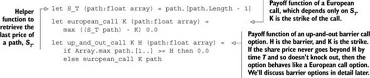
Note that in each of the payoff functions in listing 3, the path parameter appears at the rightmost position, after all contract parameters. You do this because you want the Monte Carlo simulation code to be generic, meaning you want to be able to price as many different types of payoff functions as possible. You’ll use the function-currying feature of F# to apply only contract parameters to a payoff function so that you get a curried function that maps a path (represented by a float array) to a real-valued payoff (represented by a float). Then you pass in this curried function to the Monte Carlo code to draw a large number of samples of Y.

The next listing shows the simulate_payoffs function, which is responsible for generating M simulated payoffs—that is, M samples of Y.

Listing 4. simulate_payoffs function

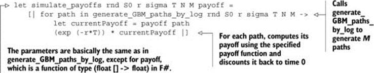
Although the function is called simulate_payoffs, it returns an array of “discounted” payoffs, because you multiply each payoff by the discounting factor exp(-r*T).

You may be wondering why we chose to discount each individual payoff sample rather than take their average first and then discount the average. Yes, it should run faster and give the same result if you factor out the discounting factor. The reason we chose to discount each sample before taking their average is that it’s easier to measure the accuracy of the Monte Carlo simulation, as covered in more detail later in this chapter.

The simulate_payoffs function will generate the samples in the numerator of Ĉ_M, so what’s left is to take an average of those samples. And that’s the purpose of the price_option function.

Listing 5. price_option function

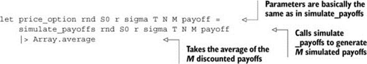
The output of the price_option function is exactly Ĉ_M. Now you’re ready to price some options. Let’s start with a European call option on a stock with strike K = 100.0 and expiry T = 0.25 years. The dynamics of the stock follow a GBM with spot price S_t0 = 100.0, an interest rate of r = 2%, and annualized volatility of σ = 40%. For Monte Carlo simulation, you need to choose N (how many data points to sample in a path) and M (how many paths to simulate).

A European call is a typical example of non-path-dependent options, so you need to simulate only the final share prices—that is, the share prices at expiry—and therefore you can set N = 1. For M, let’s start with M = 10,000. You can then run the simulation in FSI as follows:

let K, T = 100.0, 0.25

let S0, r, sigma = 100.0, 0.02, 0.40

let N, M = 1, 10000

let rnd = new System.Random()

let payoff = european_call K

let C = price_option rnd S0 r sigma T N M payoff

The C value on the last line is a draw of the random variable Ĉ_M. After running the code snippet, the option price C should be around 8.11849. How precise is this pricing result? Fortunately you can use the famous Black–Scholes pricing formula^[7] for this European call scenario. If you substitute in all the parameters, including K, T, S0, r, and sigma, to the formula, the theoretic, correct option price C should be $8.19755. The difference is about $0.079.

⁷ See “Black–Scholes model,” Wikipedia, http://en.wikipedia.org/wiki/Black-scholes.

To improve the accuracy of the simulation, what should you do? In this case, because the call option you’re looking at relies only on the final share price, increasing N doesn’t help. But as implied by the strong law of large numbers, increasing M does help improve the accuracy of the simulation results. Let’s try different Ms from 10,000 to 10,000,000 and compare the simulation results to the theoretic price C:

The results show a clear trend that Ĉ_M does get closer to the true price C as you increase M, which is consistent with our expectation. Because an analytic formula exists for pricing a European call on a stock following GBM dynamics, and it can compute the true price in no time, you don’t need to run a CPU-and-memory-bound application like a Monte Carlo simulation to price the call option. But it’s good practice to start out with something whose true price you do know, so you can use it as a sanity check to see if your Monte Carlo code works as expected.

In this example, you measure the simulation accuracy by taking the absolute difference between Ĉ_M and C, because you knew the true value of C. But more often than not, you’ll have scenarios where there’s no analytic solution available, and numerical methods like Monte Carlo simulation are the only means to compute or approximate C. In such cases, you typically don’t know the true value of C and can’t compute the difference. How do you measure simulation accuracy in those cases? Let’s discuss this topic in the next section.

Analyzing Monte Carlo estimates using variance

As mentioned, in general you can’t directly measure the difference between a Monte Carlo estimate Ĉ_M and the true value C. What else can you do to measure the accuracy of Ĉ_M? Recall that the Monte Carlo estimate Ĉ_M itself is a random variable, so you observe a different value of Ĉ_Mevery time you run a new simulation, even if all the parameters remain the same. But you want the range of the values coming out of Ĉ_M to be in some sense as narrow as possible. One of the ways to achieve that is to increase M. When M is large, you’ll probably observe that the first few digits of the values drawn out of Ĉ_M are somewhat stabilized—that is, they almost don’t change. How do you measure the “narrow-ness”?

The answer is the standard error of Ĉ_M, which is the square root of the variance estimate of Ĉ_M. Let ε_M and Var(Ĉ_M) denote the standard error and variance estimate of Ĉ_M, respectively. Then ε_M and Var(Ĉ_M) can be computed as follows

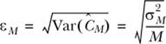
where

Basically, is nothing but the sample variance of the random variable Y (the discounted payoff). Before we delve into any more theoretical discussions, let’s see how to enhance the price_option function you wrote in the previous section to compute and the standard error ε_M. The following listing shows the new version of price_option.

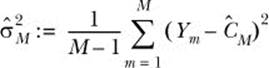
Listing 6. price_option_v2 function

With the new price_option_v2 function, run the test with the same parameters you used the previous section. The only difference is that this time you’ll use price_ option_v2 instead of price_option. The following table shows the new output from the price_option_v2function. (We didn’t fix the seed of System.Random(), so the results of the option prices will differ slightly from those in the previous section.)

When M is large enough, approaches the true variance of _Y, which is a constant that’s usually unknown; therefore you need to estimate it by . Unlike ε_M, the expectation of doesn’t depend on M. As you can see from the table, the observed values of stay close to the same level across different Ms, whereas ε_M shrinks at a rate of √10 when you increase M by 10 times. The point is that if you view as a constant (in an approximate sense), then Var(Ĉ_M) is a constant divided by M. As such, when M gets larger, the standard error ε_M gets smaller. This explains why a large M can help improve the accuracy of Monte Carlo simulation.

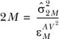
You can see that the time cost of improving accuracy by increasing M is high. If you want to reduce the standard error by one digit, you have to run 100 more simulations by comparing M = 10,000 to M = 1000,000 and M = 100,000 to M = 10,000,000. Therefore, it’s natural for researchers to come up with alternatives to reduce standard error. Instead of manipulating M, the denominator of Var(Ĉ_M), those alternatives tweak the numerator, . They reformulate Y in such a way that the expectation of Ĉ_M remains the same but the theoretic variance of Y becomes smaller. As a result, both and the standard error ε_M also get smaller. Those alternatives are known as variance-reduction techniques. You’ll see a variance-reduction technique used in a later section, but let’s first try to price other types of stock options.

Pricing path-dependent options

In this section, we’ll explore Asian options and barrier options. These options are all European style, meaning they make only one payment at expiry to the option holder and have no early-exercise feature. They’re considered path-dependent, because, unlike European call options, their final payoffs depend on not only the final price of the underlying but also the prices observed at a set of prespecified intermediate times between now and expiry. Even if two paths end up at the same final price, any discrepancies at prespecified observation times could result in very different payoffs at expiry.

Pricing Asian options

First let’s discuss Asian options. The word Asian here means that option payoffs involve averaging observed prices. There are quite a few variants of Asian options, and we have to be very specific about what Asian option we’re discussing in this section. Assume that today is the first day of the month, and you’re considering a particular Asian call option on a GBM underlying S with expiry T, strike K, and payoff as follows:

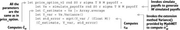
If you assume T = 0.25 years (3 months), the payoff at expiry averages three monthly close prices^[8] and takes the positive part of the average minus fixed strike K. As you might expect, unlike pricing a European call, to price this particular Asian option you have to simulate not only the final price at time _t3 but the two prices at times t₁ and t₂. Based on the code you’ve seen so far, how do you make sure you simulate the average of prices at the three time points? The easiest way is probably to set N = 3 (so that Δt = T/3) and code the Asian payoff function as shown next.

⁸ In reality, the observation times may or may not be equally spaced within the option’s life. But it’s not difficult to change your code to handle unevenly spaced observation times.

Listing 7. asian_call function

You’re ready for testing. Price the Asian call using the following parameters: S_t0 = 100, r = 2%, σ = 40%, T = 0.25, K = 100, N = 3, and M = 10,000,000. These parameters are much the same as the ones you’ve been using so far, except that now you set N = 3. The F# code for the Asian call test is as follows:

> let K, T = 100.0, 0.25

let S0, r, sigma = 100.0, 0.02, 0.4

let N, M = 3, 10000000

let rnd = new System.Random()

let payoff = asian_call K;;

(...)

> let (C,Y_var,std_error) = price_option_v2 rnd S0 r sigma T N M payoff

;;

Real: 00:00:22.677, CPU: 00:00:22.323, GC gen0: 984, gen1: 223, gen2: 1

val std_error : float = 0.00295

val Y_var : float = 86.75458

val C : float = 5.88672

The simulation says that the Asian option is worth about $5.88672 as of today. How do you verify this pricing result? Unfortunately, there’s currently no close-form solution available for computing true prices of arithmetic averaging Asian options. Although you can’t know the true price for certain, academic research over the past two decades has provided analytic formulas for approximating the true price or inferring tight lower or upper bounds.

Another validation technique involves comparing the simulation results with the ones computed by other numerical methods, such as finite difference methods. Although we can’t go into depth on the topic of analytic approximation or other numerical methods, there’s still one simple sanity check you can do. If you compare the results of the Asian call to the prices of the European call you computed in the previous section, you can see that they share the same parameters. But due to the averaging nature, the price of the Asian call should be smaller than that of the European call—which is the case, as you can see from the numerical results.

Pricing barrier options

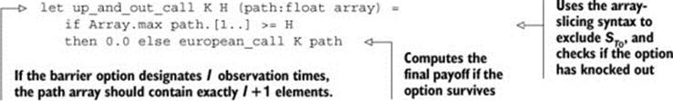
Now let’s move on to barrier options. There are quite a few different types of barrier options. Our example is an up-and-out barrier option with discrete observation times, meaning the option contract designates a barrier H and a finite set of times; at each time, the underlying price is observed to determine if the price has reached or gone beyond H.

If the stock price reaches or exceeds H, the option is worthless and terminates immediately, which constitutes a knock-out event. If the option survives all observation times, it pays a European call payoff at expiry. Assume that this example is a newly issued barrier option with expiry T = 0.25years = 3 months, a monthly observation schedule of , barrier H = 125, and strike K = 100. Therefore, the option’s payoff can be expressed as follows:

The option pays nothing if S_ti ≥ H for any t_i, otherwise it pays (S_T – K)⁺ at time T.

As in the previous Asian option example, you need to sample at three time points in each price path. These three time points are equally spaced, so you need to set N = 3. Earlier, listing 3 showed a few payoffs in F#, and one of them was for the barrier option. For convenience, let’s isolate the barrier option payoff in the next listing and discuss it in greater detail.

Listing 8. up_and_out_call function

As with the Asian call earlier, listing 8 uses these parameters: S_t0 = 100, r = 2%, σ = 40%, T = 0.25, K = 100, N = 3, and M = 10,000,000, along with a barrier parameter, H = 125. The F# code for the up-and-out barrier call test is as follows:

> let K, T = 100.0, 0.25

let S0, r, sigma = 100.0, 0.02, 0.4

let N, M = 3, 10000000

let H = 125.0

let rnd = new System.Random()

let payoff = up_and_out_call K H;;

(...)

> let (C,Y_var,std_error) = price_option_v2 rnd S0 r sigma T N M payoff;;

Real: 00:00:23.785, CPU: 00:00:22.557, GC gen0: 905, gen1: 263, gen2: 3

val std_error : float = 0.00194

val Y_var : float = 37.58121

val C : float = 3.30157

Similar to Asian options, there’s currently no analytic formula for discretely monitored barrier options, so you can’t compare the pricing result to a true answer. Closed-form solutions for continuously monitored barrier options do exist, which you can apply together with the BGK barrier-adjustment formula to approximate the prices of discretely monitored barrier options. Also, a barrier call option should be cheaper than a European call option with the same parameters (except the barrier). In addition, you can set an extremely high barrier relative to the spot price S_t0 so that it’s almost impossible for the barrier option to knock out. In this case, an up-and-out barrier call behaves like a European call.

Up-and-in barrier call

You can modify listing 8 to implement the payoff function for up-and-in barrier calls. As its name suggests, an up-and-in barrier call pays nothing at expiry if the price of the underlying stock never exceeds the barrier H; otherwise, it behaves like a European call. When pricing an up-and-in barrier call, keep in mind that a portfolio of one up-and-in and one up-and-out should behave like a European call, provided that both the up-and-in and up-and-out share the same strike, barrier, and expiry.

Variance reduction using antithetic variates

So far you’ve used the ordinary Monte Carlo estimate to price a European call option, an Asian call option, and an up-and-out barrier call option. You also computed their standard errors—the square root of the simulation variance. As mentioned earlier, in addition to increasing the number of simulation trials, you can take advantage of variance-reduction techniques, which may reduce simulation variance without having to increase the number of trials. Let’s explore the antithetic variates (AV) method, which is widely adopted in the industry.

Recall that for m = 1,2,...,M, in order to sample Y_m, the _mth draw of discounted payoff Y, you have to sample a price path x_m, which is determined by a vector of draws from Brownian motion W. Let denote the vector. Then you can say that Y_m is ultimately a function of Z_m. Using the AV method, you follow these steps:

1. Generate M samples of Z_m. For each Z_m sample, negate each of its elements. Let be the negated vector.

2. For each pair of Z_m and , generate two paths, x_m and respectively.

3. For each pair of x_m and , compute discounted payoffs Y_m and , respectively.

4. For each pair of Y_m and , take the average of them. Let .

5. As in the ordinary Monte Carlo method, take the average of all samples, which is the AV Monte Carlo estimate for the true price. Let .

Next let’s compare the AV method and the ordinary Monte Carlo method in terms of expectation and variance. As you can see from the previous steps, in order to compute , you use 2M paths, although half of them are deliberately set up and thus negatively correlated to the other half. As such, it may be fairer or make more sense to compare against Ĉ_2M instead of Ĉ_M.

Now let’s look at expectation and variance of the AV estimate . It can be mathematically proven that , so the AV estimate , like the ordinary estimate Ĉ_2M, is also an unbiased estimate for the true price _C. As for how the AV estimate can reach a smaller standard error or equivalently a lower variance, the reasoning is that because Z_m and are negatively correlated, we hope^[9] Y_m and are also negatively correlated; the negative correlation between Y_m and can make the variance of smaller than that of Y_m, and as a result, Var() should be less than Var(Ĉ_2M), which is our ultimate goal.

⁹ Why “hope” here? Because the negative correlation between Z_m and alone isn’t sufficient to guarantee that Y_m and are also negatively correlated. The correlation between Y_m and is also determined by the shape of the payoff function we’re considering. If the payoff function is symmetric, applying the AV method may lead to a worse result—that is, Var() > Var(Ĉ_2M).

To implement the AV method, you need to revise three of the functions: generate_GBM_paths_by_log, simulate_payoffs, and price_option_v2. The following listing shows the new version of generate_GBM_paths_by_log.

Listing 9. generate_GBM_paths_by_log_AV function

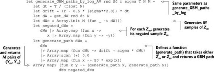
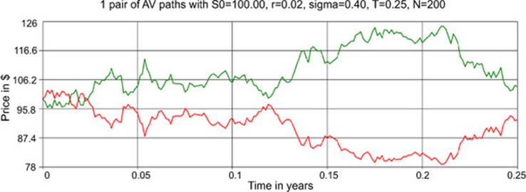
So the generate_GBM_paths_by_log_AV function implements steps 1 and 2 of the AV method. You can then invoke it to generate a pair of AV paths and plot them like the chart in figure 2. The green and red paths are generated based on Z₁ and respectively; the colors aren’t visible in the printed book, but the Z₁-based path is higher than the -based path for all but the first 0.25 years. The paths look negatively correlated, as expected.

Figure 2. An example of using the generate_GBM_paths_by_log_AV function to generate one pair of AV paths

The next listing shows the new versions of the other two functions, simulate_ payoffs and price_option_v2.

Listing 10. simulate_payoffs_AV and price_option_v2_AV

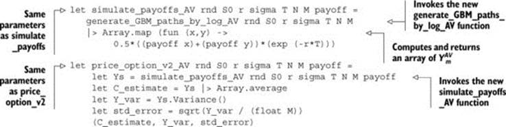
As you can see in listing 10, there aren’t many changes to the regular simulate_payoffs and price_option_v2 functions. The new versions implement steps 3, 4, and 5 of the AV method. Before you test the AV code, let’s summarize the numerical results that you received in the previous sections using the regular estimate Ĉ_2M. Let M be 5,000,000, so 2M = 10,000,000 is exactly the number of paths you used previously:

Now let’s apply the new AV estimate to the same options. Here are the results:

By comparing these two tables, you can observe the following:

· For option prices, both the regular estimate and the AV estimate produce much the same results.

· For standard error ε, improves by 15–22% against ε_2M. (Take the European call as an example: 100% – (0.00332/0.00421) × 100% = 21.14%.)

You may also notice that the AV estimate took about 10% more time to compute compared to the regular estimate. Therefore, you may feel that the AV estimate didn’t do a good job, because you might suppose that if you chose to increase the number of paths for Ĉ_2M by 10%, simulation accuracy of the regular estimate in terms of standard error would probably be as good as or only slightly worse than that of the AV estimate. In other words, you might think the AV estimate could do better because it took more time.

Let’s interpret the two tables in another way by answering the following question: if you want ordinary estimate Ĉ_2M to achieve the same level of standard error as , how many paths do you have to generate? You can estimate the answer using the following formula:

This formula involves nothing but rearranging the definition of standard error, which we discussed earlier. Let’s take the European call as an example: 2M = 177.40473/(0.00332 × 0.00332) = 16,094,928, so you need 60% ((16,094,928 – 10,000,000)/ 10,000,000 ≅ 60%) more paths, and thus roughly 60% more runtime, to match the accuracy of the AV estimate. If you do the same calculation for Asian and barrier calls, you’ll see that you need 66% and 41% more paths, respectively. As a result, you’ll see that the AV method does a good job in terms of reducing simulation variance.

Replacing GBM with the Heston model

In this chapter, we use GBM to model the dynamics of share prices. But GBM can’t produce volatility skews and thus isn’t realistic enough. In plain English, this means GBM can’t explain a phenomenon in the market (or a common perception in people’s mind): “The bull walks up the stairs; the bear jumps out the window.” This issue can be addressed by local volatility models or stochastic volatility models.

The Heston (1993) model is one of the stochastic volatility models used in the industry. As the name suggests, it allows the volatility σ to be stochastic—that is, the volatility σ has its own dynamics. In most cases, the dynamics of σ is set to be negatively correlated with the dynamics of share price, so that when you see a large volatility, it’s more likely to be used to have the share price go down rather than up. If you’re interested in implementing the Heston model, a good book to consult is Monte Carlo Methods in Financial Engineering by Paul Glasserman (Springer, 2003). Note that you need to know how to draw correlated bivariate normals in order to simulate Heston dynamics.

Summary

This chapter explored Monte Carlo simulation. You learned how to write F# code to compute a Monte Carlo estimate, analyze its accuracy, and improve accuracy by using a variance-reduction technique. Monte Carlo simulation is widely used in science and engineering, so the concepts and techniques we discussed are applicable not only to finance but to many other areas as well.

In this chapter, you simulated stock-price paths and derivative payoffs. You saw how higher-order functions and function currying can help you write generic code to price different types of derivatives. Furthermore, F#’s built-in support for pipelining and array processing can make your code more concise and expressive. Compared to other advanced features of F# you’ll learn in this book, the functional features used in this chapter are relatively basic but can prove handy when you’re writing code for numerical computations.

About the author

Chao-Jen Chen is a quantitative analyst at the fixed income trading desk of an insurance company and an instructor in the Financial Mathematics Program of the University of Chicago’s Preparation Course held at its Singapore Campus. He teaches calculus, probability, linear algebra, and MATLAB with a focus in finance. He’s also a senior teaching assistant in the Financial Mathematics Program, mainly responsible for running review classes for courses, including option pricing, numerical methods, and computing in F# and C++. Previously, he worked at the Structured Trade Review group of Credit Suisse AG, where he was the team lead of the Emerging Market sector and was responsible for the verification of model appropriateness and trade economics for all structured products traded in emerging markets, including structured loans, credit derivatives, fixed income derivatives, and foreign exchange derivatives.

Chao-Jen holds an undergraduate degree in mathematics (National Tsing Hua University) and postgraduate degrees in industrial engineering (National Taiwan University) and financial mathematics (University of Chicago). He has a long-term interest in computer programming, operations research, and quantitative finance. Chao-Jen writes a blog at http://programmingcradle.blogspot.com, and he can be reached via email at ccj@uchicago.edu.