Practical Reverse Engineering: x86, x64, ARM, Windows Kernel, Reversing Tools, and Obfuscation (2014)

Chapter 5. Obfuscation

Reverse engineering compiler-generated code is a difficult and time-consuming process. The situation gets even worse when the code has been hardened, deliberately constructed to resist analysis. We refer to such techniques for hardening programs under the general umbrella of obfuscation. Some examples of situations in which obfuscation might be applied are as follows:

· Malware—Avoiding the scrutiny of both antivirus detection engines and reverse engineers is a primary motive of the criminals who employ malware in their operations, and therefore this has been a traditional application of obfuscation for many years now.

· Protection of intellectual property—Many commercial programs have some sort of protection against unauthorized duplication. Some systems employ further obfuscation for the purpose of obscuring the implementation details of certain parts of the system. Good examples include Skype, Apple's IMessage, or even the Dropbox client, which protect their communication protocol formats with obfuscation and cryptography.

· Digital Rights Management—DRM schemes commonly protect certain crucial pieces of information (e.g., cryptographic keys and protocols) using obfuscation. Apple's FairPlay, Microsoft's Media Foundation Platform and its PlayReader DRM, to cite only two, are examples of obfuscation application. Currently, this is the leading contemporary application of obfuscation.

Speaking in the abstract, “obfuscation” can be viewed in terms of program transformations. The goal of such methods is to take as input a program, and produce as output a new program that has the same computational effect as the original program (formally speaking, this property is calledsemantic equivalence or computational equivalence), but at the same time it is “more difficult” to analyze.

The notion of “difficulty of analysis” has long been defined informally, without any backing mathematical rigor. For example, it is widely believed that—insofar as a human analyst is concerned—a program's size is an indicator of the difficulty in analyzing it. A program that consumes 20,000 instructions in performing a single operation might be thought to be “more difficult” to analyze than one that takes one instruction to perform the same operation. Such assumptions are dubious and have attracted the scrutiny of theoreticians (such as that by Mila Dalla Preda¹⁷ and Barak et al.²).

Several models have been proposed to represent an obfuscator, and (in a dual way) a deobfuscator. These models are useful to improve the design of obfuscation tools and to reason about their robustness, through adapted criteria. Among them, two models are of special interest.

The first model is suited for the analysis of cryptographic mechanisms, in the so-called white box attack context. This model defines an attacker as a probabilistic algorithm that tries to deduce a pertinent property from a protected program. More precisely, it tries to extract information other than what can be trivially deduced from the analysis of the program's inputs and outputs. This information is pertinent in the sense that it enables the attacker to bypass a security function or represents itself as critical data of the protected program. In a dual way, an obfuscator is defined in this model as a virtual black box's probabilistic generator, an ideal obfuscator ensuring that the protected program analysis does not provide more information than the analysis of its input and output distributions.

Another way to formalize an attacker is to define the reverse engineering action as an abstract interpretation of the concrete semantics of the protected program. Such a definition is naturally suited to the static analysis of the program's data flow, which is a first step before the application of optimization transformations. In a dual way, an obfuscator is defined in the abstract interpretation model as a specialized compiler, parameterized by some semantic properties that are not preserved.

The goal of these modeling attempts is to get some objective criteria relative to the effective robustness of obfuscation transformations. Indeed, many problems that were once thought to be difficult can be efficiently attacked via judicious application of code analysis techniques. Many methods that have arisen in the context of more conventional topics in programming language theory (such as compilers and formal verification) can be repurposed for the sake of defeating obfuscation.

This chapter begins with a survey of existing obfuscation techniques as commonly found in real-world situations. It then covers the various available methods and tools developed to analyze and possibly break obfuscation code. Finally, it provides an example of a difficult, modern obfuscation scheme, and details its circumvention using state-of-the-art analysis techniques.

A Survey of Obfuscation Techniques

For simplicity of presentation, we begin by dividing obfuscations into two categories: data-based obfuscation and control-based obfuscation. You will see later that the two combine in complex and difficult ways and are, in fact, inseparable. Before wandering deeply down these paths, however, we begin with a representative example of the types of code that one might encounter in real-world obfuscation. Note that the example is particularly simple because it involves only data-based obfuscations, not control-based ones.

The Nature of Obfuscation: A Motivating Example

When targeting the x86 processor, compilers tend to generate instructions drawn from a particular, tiny subset of the available instruction set, and the control structure of the generated program follows predictable conventions. Over time, the reverse engineer develops a style of analysis tailored to these patterns of structured code. When confronted by nonconformant code, the speed of one's analysis can suffer tremendously.

This phenomenon can be illustrated simply by a concrete example. Because one of the goals of a compiler optimizer is to reduce the amount of computational resources involved in performing a task, and 50 years' worth of research have imbued them with formidable capabilities toward this pursuit, one does not commonly spot obvious inefficiencies in the translation of the original source code into assembly language. For example, if the source code were to dictate that some variable be incremented by five (e.g., due to a statement such as x += 5;), a compiler would likely generate assembly code akin to one of the following:

01: add eax, 5

02: add dword ptr [ebp-10h], 5

03: lea ebx, [ecx+5]

In obfuscated code, one might instead encounter code such as the following, assuming that EAX corresponds to the variable x, and that the value of EBX is free to be overwritten (or “clobbered”):

01: xor ebx, eax

02: xor eax, ebx

03: xor ebx, eax

04: inc eax

05: neg ebx

06: add ebx, 0A6098326h

07: cmp eax, esp

08: mov eax, 59F67CD5h

09: xor eax, 0FFFFFFFFh

10: sub ebx, eax

11: rcl eax, cl

12: push 0F9CBE47Ah

13: add dword ptr [esp], 6341B86h

14: sbb eax, ebp

15: sub dword [esp], ebx

16: pushf

17: pushad

18: pop eax

19: add esp, 20h

20: test ebx, eax

21: pop eax

You can see a variety of obfuscation techniques at work in this example:

· Lines 1–3 use the “XOR swap trick” for exchanging the contents of two locations—in this case, the EAX and EBX registers.

· Line 4 shows an assignment to the EAX register that is actually “junk” (as EAX is overwritten with a constant on line 8).

· On lines 5–6, the EBX register is negated and added to the constant 0A6098326h: EBX = - EAX + 0A6098326h.

· On line 7, EAX is compared with ESP. The CMP instruction modifies only the flags, and the flags are overwritten on subsequent lines before being used again, so this code is junk.

· Lines 8–9 move the constant 59F67CD5h into the EAX register and XOR it with -1h (which, in binary, is all one bits). XORing with all ones is equivalent to the NOT operation; therefore, the effect of this sequence is to move the constant 0A609832Ah into EAX.

· Line 10 subtracts the constant in EAX from EBX: EBX = - EAX + 0A6098326h - 0A609832Ah, or EBX = - EAX - 5, or EBX = -( EAX + 5).

· Line 11 modifies EAX through use of the RCL instruction. This instruction is junk because EAX is overwritten on line 18.

· Lines 12–13 push the constant 0F9CBE47Ah and then add the constant 6341B86h to it, resulting in the value 0h on the bottom of the stack.

· Line 14 modifies EAX through use of the SBB instruction, involving the extraneous register EBP. This instruction is junk, as EAX is overwritten on line 18.

· Line 15 subtracts EBX from the value currently on the bottom of the stack (which is 0h). Therefore, dword ptr [ESP] = 0 - -( EAX + 5), or dword ptr [ESP] = EAX + 5.

· Lines 16–19 demonstrate operations involving the stack: nine dwords are pushed, one is popped into EAX, and the stack pointer is then adjusted to point to the same location that it pointed to before the sequence executed.

· Line 20 tests EBX against the EAX register and sets the flags accordingly. If the flags are redefined before their next use, then this instruction is dead.

· Line 21 pops the value on the bottom of the stack (which holds EAX + 5) into the EAX register.

In summary, the code computes EAX = EAX + 5.

Needless to say, the obfuscated code does not at all resemble the compiler-generated code, and one faces considerable difficulty in ascertaining the functionality of the snippet. Several obfuscation techniques are present in this example:

· Pattern-based obfuscation

· Constant unfolding

· Junk code insertion

· Stack-based obfuscation

· The use of uncommon instructions, such as RCL, SBB, PUSHF, and PUSHAD

Correspondingly, a variety of existing compiler transformations can be used to render the code into a form that is closer to the original:

· Peephole optimization

· Constant folding

· Dead statement elimination

· Stack optimization

The Interplay Between Data Flow and Control Flow

Consider the following instruction sequence:

01: mov eax, dword ptr [ebp-10h]

02: jmp eax

Suppose you wish to construct a “correct,” classical control-flow graph for a program containing sequences like this one. In order to determine what the next instruction will be after line 2 has executed—or, perhaps the set of potential successor instructions—you need to determine the set of possible value(s) for the EAX register at that location. In other words, the control flow for this snippet is dependent upon the data flow as it pertains to the location [EBP-10h] at the program point l1 (line 1). However, in order to determine the data flow with respect to [EBP-10h], you need to determine the control flow with respect to the line 1 location: You must know all possible control transfer instructions (and the associated data flow leading to those locations) that could possibly target the line 1 location. It is not meaningful to talk about control flow without simultaneously talking about data flow, or vice versa.

The situation is even more difficult than it might appear on the surface. Program analysis tries to answer questions such as “What values might the location [EBP-10h] assume under any possible circumstance?” To combat intractability and undecidability, many forms of program analysis employ approximations of the state space. Some approximations are fine (e.g., approximating the set {1,3} by {1,2,3} ), and some are coarse (e.g., approximating that same set by {0,1,…,2³² −1}). (Fine and coarse are not technical terms in this paragraph.) If you cannot finely approximate the set of potential values of the [EBP-10h] location (for example, if you must assume that the location could take on any possible value), then you do not know where the jump will point, so you must assume that it could target any location within the address space. Then, the data flow facts from the line 2 location must be propagated into those at every other location. In practical settings, such a decision will severely impact the analysis, most likely causing it to conservatively conclude that all states are possible at all locations, which is correct but useless.

Worse yet, if you ever must assume that a jump could target any location, then due to variable-length instruction encoding on x86, many of these transfers will be into locations that do not correspond to the beginning of a proper instruction. Such bogus instructions are likely to wreak havoc on any analysis, especially when combined with the observations in the previous paragraph.

Academic work in this area, such as that by Kinder³⁰ and Thakur et al.⁴¹, seeks to construct systems that can return correct answers for all possible inputs. These systems prefer to tell users that they cannot determine precise information, return correct but grossly imprecise results, or die trying (e.g., by exhausting all available memory or failing to terminate due to tractability issues), rather than give an answer that is not fully justified. This goal is laudable, given the motivation from whence these disciplines were founded: to ensure absolute correctness of programs and analyses. However, it is not in line with our motivations as obfuscation researchers.

Deobfuscation is a creature of a different sort than formal verification or program analysis, even if we prefer to use techniques developed in those contexts. Whereas an obfuscator transforms a program P_orig into a program P_obf, we seek either a translator from P_obf into P_orig or enough information about P_obf to answer questions proximate to some reverse engineering effort. We hesitate to use unsound methods, but we prefer actual results when the day is finished, so we may employ such methods, albeit consciously and grudgingly.

Data-Based Obfuscations

We begin by looking at obfuscation techniques that can be best described in terms of their effect on data values and noncontrol computations. In particular, assume that the presented snippets occur within a single basic block of the program's control-flow graph. The discussions of control-based obfuscations, and their combination with data-based obfuscations, are deferred to later sections.

Constant Unfolding

Constant folding is one of the earliest and most basic compiler optimizations. The goal of this optimization is to replace computations whose results are known at compile-time with those results. For example, in the C statement x = 4 * 5;, the expression 4 * 5 consists of a binary arithmetic operator (*) that is supplied with two operands whose values are statically known (4 and 5, respectively). It would be wasteful for the compiler to generate code that computed this result at run-time, as it can deduce what the result will be during compilation. The compiler can simply replace the assignment with x = 20;.

Constant unfolding is an obfuscation that performs the inverse operation. Given a constant value that is used somewhere in the input program, the obfuscator can replace the constant by some computation process that produces the constant. You have already encountered this obfuscation in the motivating example:

01: push 0F9CBE47Ah

02: add dword ptr [esp], 6341B86h

Neglecting the modifications that this sequence has upon the flags, this was found to be equivalent to push 0h.

Data-Encoding Schemes

The fundamental flaw of this technique is that constants have to be dynamically decoded (thus exposed, as well as the decode function) at run-time before being processed. We have the encoding function f(x) = x − 6341B86h, whose result f(x) is pushed on the stack, and then the decoded function is applied: f_{- 1} (x)= x + 6341B86h. This construct is trivial; deobfuscation is done by simply applying the standard compiler's constant folding optimization.

Efforts have been made to harden these statements and propose more resilient encoding schemes. Some techniques, such as polynomial encoding and residue encoding, have been described in patent US6594761 B1 by Chow, Johnson and Gu¹¹. Affine maps are also commonly used.

What if one could find an encoding such that it is not mandatory to decode variables to manipulate them (an equivalent operation can be defined on the encoded variables)? This property, called homomorphism, has been discussed in an obfuscation-oriented view, as well as a refinement of the residue coding technique in works such as those of Zhu and Thomborson.⁴⁴

In abstract algebra, a homomorphism is an operation-preserving mapping between two algebraic structures. Consider, for example, two groups, G and H, equipped respectively with operations +_g and +_h. We want to construct a mapping f between the sets underlying G and H, and we want your mapping to respect the operations +_g and +_h. In particular, we must have that f (x+_g y) = f(x) +_h f(y).

The notion of a homomorphism can be generalized beyond groups to arbitrary algebraic structures. For example, you can consider ring homomorphisms that simultaneously preserve both the addition and the multiplication operators. In contrast to mappings that preserve only one of the ring's operations and not the other, or induce restrictions upon the operators or their usage, unrestricted mappings are considered fully homomorphic.

Fully homomorphic mappings have a natural application to obfuscation. If the source algebra is the unencoded domain, and the target algebra is the encoded one, then a homomorphic mapping enables us to perform computations directly upon the encoded data without having to decode it beforehand and re-encode it afterward.

At the time of writing, the topic of homomorphic cryptography is still in its infancy. Fully homomorphic cryptosystems have been shown to exist, and they enable the computation of encrypted programs upon encrypted data. That is to say, rigorous statements can be made concerning the hardness of determining specifics about the program being executed, and which data it is operating upon. At present, the schemes are too inefficient for practical usage, and how to best apply the technology to arbitrary computer programs is an open question.

Dead Code Insertion

Another common compiler optimization is known as dead code elimination, which is responsible for removing program statements that do not have any effect on the program's operation. For example, consider the following C function:

int f()

{

int x, y;

x = 1; // this assignment to x is dead

y = 2; // y is not used again, so it is dead

x = 3; // x above here is not live

return x; // x is live

}

Ultimately, the function returns the number 3. It does so after several meaningless computations that do not affect the function's output. The first assignments to x and y are said to be dead, as they have no effect on live computations.

Obfuscators perform the inverse of this operation by inserting dead code for the purpose of making the code harder to follow—the reverse engineer has to manually decide whether a given instruction participates in the computation of some meaningful result. The ability to insert “dead” code requires the obfuscator to know which registers are “live” at every given program point; for example, if EAX contains an important value (it's live), and EBX does not (it's dead), then you can insert statements that modify EBX.

Deobfuscation of this construct is done by simply applying the standard compiler's dead statement elimination optimization, which can be done either on a single basic block or across an entire control-flow graph.

Arithmetic Substitution via Identities

Mathematical statements can be made relating the results of certain operators to the results of combinations of other operators. You have already seen an instance of this general phenomenon in the motivating example, when you encountered the instruction XOR EAX, 0FFFFFFFFh (where the binary representation of 0FFFFFFFFh is all one bits). Because 0 XOR 1 = 1, and 1 XOR 1 = 0, this instruction actually flips each of the bits in EAX; in other words, it is synonymous with the NOT operator. Similarly, you can make the following statements:

· -x = ˜x + 1 (by definition of two's complement)

· rotate left(x,y) = (x y) | (x (bits(x)-y))

· rotate right(x,y) = (x y) | (x (bits(x)-y))

· x-1 = ˜-x

· x+1 = - x

Pattern-Based Obfuscation

Pattern-based obfuscation, a staple of many contemporary protections, has a simple underlying concept. The protection author manually constructs transformations that map one or more adjacent instructions into a more complicated sequence of instructions that has the same semantic effect. For example, a pattern might convert the sequence

01: push reg32

into this sequence (which we will call #1):

01: push imm32

02: mov dword ptr [esp], reg32

Or, it might convert that same sequence into this sequence (#2):

01: lea esp, [esp-4]

02: mov dword ptr [esp], reg32

Or this one (#3):

01: sub esp, 4

02: mov dword ptr [esp], reg32

Patterns can be arbitrarily complicated. A more complex example might substitute the pattern:

01: sub esp, 4

for this pattern (#4):

01: push reg32

02: mov reg32, esp

03: xchg [esp], reg32

04: pop esp

Some protections have hundreds of patterns. Most protections apply patterns randomly to the input sequence, such that two obfuscations of the same piece of code result in a different output. Also, the patterns are applied iteratively. Consider the following input:

01: push ecx

Imagine that it is transformed via substitution #3:

01: sub esp, 4

02: mov dword ptr [esp], ecx

Now suppose that the obfuscator is run a second time, and the first instruction is replaced according to pattern #4:

01: push ebx

02: mov ebx, esp

03: xchg [esp], ebx

04: pop esp

05: mov dword ptr [esp], ecx

This process can be applied indefinitely, resulting in an arbitrarily large output sequence. With enough patterns, one can transform one instruction into millions of instructions.

Note a few things about these substitutions. #1 and #2 preserve semantic equivalence: After those sequences execute, the CPU will be in the same state that it would have been if the original one were executed instead. #3 does not preserve semantic equivalence, because it uses the sub-instruction that changes the flags, whereas the original push does not. As for sequence #4, the original does change the flags, whereas the substitution does not; also, whereas the original does not modify memory at all, the substitution writes the value of ESP onto the bottom of the stack (hence, you could also consider this as being equal to the PUSH ESP instruction).

These considerations illustrate the difficulty of obfuscating assembly code post-compilation. The protection is only safe to execute substitution #3 if it is known that the flags modified by the instruction are not used before the next modification to those flags. Substitution #4 is similarly safe if the flags are dead, and if the resultant code is indifferent to the contents of [ESP] after the original SUB ESP, 4 operation. Ensuring flag liveness requires building the function's control-flow graph, which can be difficult due to indirect branches. Ensuring that the stack memory modification is safe would be extremely difficult due to memory aliasing. These specific concerns are unlikely to affect normal functions generated by a compiler for which control-flow graphs can be generated, but it is hoped that they illustrate the perils of applying semantically non-equivalent transformations to compiled code.

Owing to the complexities of obfuscating compiled assembly language, protections most commonly apply these transformations against the code corresponding to the protection itself, rather than the target's code. This way, the protection authors can guarantee that the input code will be oblivious to those transformations that do not preserve strict semantic equivalence.

Deobfuscation of this type of obfuscation is simple, although it can be time-consuming to write the deobfuscator. One can construct inverse pattern substitutions, which instead map the target sequences into the original ones. In fact, this corresponds to a routine compiler optimization known aspeephole optimization. Academic works, such as that by Jacob et al.²⁵ or Bansal,¹ have discussed the automated construction of both pattern-obfuscators and peephole optimizers.

This brings us back to the question of practical results versus academic ones. Suppose you are dealing with a pattern-based obfuscator that contains errors (e.g., erroneous pattern substitutions that do not preserve semantic equivalence). Suppose further that you, as a deobfuscation researcher, are aware of the errors and are able to correct them at deobfuscation time. This means that your deobfuscator will similarly not preserve semantic equivalence and is therefore “incorrect” in absolute terms as far as transformation goes, but it actually produces “correct” results with respect to the pre-obfuscated code. Should you make the substitution? The formal correctness crowd would say no; we would answer in the affirmative.

Control-Based Obfuscation

When reverse engineering compiler-generated code, reverse engineers are able to rely on the predictability of the compiler's translations of control flow constructs. In doing so, they can quickly ascertain the control flow structure of the original code at a level of abstraction higher than assembly language. Along the way, the reverse engineer relies upon a host of assumptions about how compilers generate code. In a pure compiled program, all code in a basic block will be most often sequentially located (heavy compiler optimizations can possibly render this basic premise null and void). Temporally related blocks usually will, too. A CALL instruction always corresponds to the invocation of some function. The RET instruction, too, will almost always signify the end of some function and its return to its caller. Indirect jumps, such as for implementing switch statements, appear infrequently and follow standard schemas.

Control-based obfuscation attacks these planks of standard reverse engineering, in a way that complicates both static and dynamic analyses. Standard static analysis tools make similar assumptions as human reverse engineers, in particular:

· The CALL instruction is only used to invoke functions, and a function begins at the address targeted by a call.

· Most calls return, and if they do, they return to the location immediately following the CALL instruction; ret and RETN statements connote function boundaries.

· Upon encountering a conditional jump, disassemblers assume that it was placed into the code “in good faith”—in particular that:

· Both sides of the branch could feasibly be taken.

· Code, not data, is located down each side of the branch.

· They will be able to easily ascertain the targets of indirect jumps.

· Indirect jumps and calls will only be generated for standard constructs such as switches and function pointer invocations.

· All control transfers target code locations, not data locations.

· Exceptions will be used in predictable ways.

With respect to control transfers, disassemblers assume a model of “normality” based around the patterns of standard compiled code. They explicitly create functions at call targets, end them at return statements, continue disassembling after a call instruction, traverse both sides of all conditional branches, assume all branch targets are code, use syntactic pattern-matching to resolve indirect jump schema, and generally ignore exceptional control flow. Violating the assumptions laid out previously leads to very poor disassembly. This is a consistent thorn in the side of obfuscation researchers, and an open research topic (as discussed previously) in verification.

Dynamic analysis has an easier time with respect to indirect control transfers, since it can explicitly follow execution flow. However, the attacker still faces questions involving determining the targets of indirect transfers, and suffers from the lack of sequential locality induced by so-calledspaghetti code. The following sections elaborate upon what happens when these assumptions are challenged.

Functions In/Out-Lining

The call graph of a program carries a lot of its high-level logic. Playing with the notion of a function can break some of the reverser's assumptions. It's possible to:

· Inline functions—The code of a subfunction is merged into the code of its caller. Code size can grow quickly if the subfunction is called multiple times.

· Outline functions—A subpart of a function is extracted and transformed into an independent function and replaced by a call to the newly created functions.

Combining these two operations over a program leads to a degenerated call graph with no apparent logic. It goes without saying that functions' prototypes can also be toyed with to reorder arguments, add extra, fake arguments, and so on, to contribute to logic obscurity.

Destruction of Sequential and Temporal Locality

As stated, and as understood intrinsically by those who reverse engineer compiled code, the instructions within a single, compiled basic block lie in one straight-line sequence. This property is called sequential locality. Furthermore, compiler optimizers attempt to put basic blocks that are related to one another (for example, a block and its successors) nearby, for the purpose of maximizing instruction cache locality and reducing the number of branches in the compiled output. We call this property the sequential locality of temporally related code. When you reverse engineer compiled code, these properties customarily hold true. One learns in analyzing such code that all of the code responsible for a single unit of functionality will be neatly contained in a single region, and that the proximate control-flow neighbors will be nearby and similarly sequentially located.

A very old technique in program obfuscation is to introduce unconditional branches to destroy this aspect of familiarity that reverse engineers organically obtain through typical endeavors. Here is a simple example:

01: instr_1:

02: push offset caption

03: jmp instr_4

04:

05: instr_2:

06: call MessageBoxA

07: jmp instr_5

08:

09: instr_3:

10: push 0

11: jmp instr_2

12:

13: start:

14: push 0

15: jmp instr_1

16:

17: instr_4:

18: push offset dlgtxt

19 jmp instr_3

20:

21: instr_5:

22: ; …

This example shows the lack of sequential locality for instructions within a basic block, and not temporal locality of multiple basic blocks. In practice, large amounts of the program's code will be intertwined in such a fashion (usually with more than one instruction on a given basic block, unlike the preceding example).

From a formal perspective, this technique does not even deserve to be called “trivial,” as it has no semantic effect whatsoever on the program. Constructing a control-flow graph and removing spurious unconditional branches will defeat this scheme entirely. However, in terms of analysis performed manually by a human, the ability to follow the code has been dramatically slowed.

Processor-Based Control Indirection

For most processors, two essential displacement primitives are the JMP-like branch and the CALL-like save instruction pointer and branch. These primitives can be obfuscated by using dynamically computed branch addresses or by emulating them. One of the most basic techniques is the couple PUSH-RET used as a JMP instruction:

01: push target_addr

02: ret

That's (almost) semantically equivalent to the following:

01: jmp target_addr

The CALL instruction is an easy target for obfuscators because most disassemblers assume the following about its high-level semantics:

· The target address is a subfunction entry point.

· A call returns (i.e., the instruction after the CALL is executed).

It is actually easy to break these assumptions. Consider the following example:

01: call target_addr

02: <junk code>

03: target_addr:

04: add esp, 4

The CALL is used as a JMP; it will never return to line 2. The stack is fixed (the return address is discarded from the stack) on line 3. Next consider, these two elements:

01: basic_block_a:

02: add [esp], 9

03: ret

and

01: basic_block_b:

02: call basic_block_a

03: <junk code>

04: true_return_addr:

05: nop

basic_block_b's line 2 CALL instruction points to basic_block_a, which actually is only a stub that updates (see basic_block_a's line 2) the return address stored onto the top of the stack before the RET instruction uses it (basic_block_a's line 3). In these two examples the result is an interval between CALL's natural (expected) and effective return addresses; an obfuscator can (and will) take advantage to insert code that thwarts disassemblers and creates confusion.

The following example is an interesting enrichment of the standard PUSH-RET used as JMP previously:

01: push addr_branch_default

02: push ebx

03: push edx

04: mov ebx, [esp+8]

05: mov edx, addr_branch_jmp

06: cmovz ebx, edx

07: mov [esp+8], ebx

08: pop edx

09: pop ebx

10: ret

The basis of this construction actually is a PUSH-RET. Line 7 writes the target address onto the stack; it is used by the RET at line 10. The pushed address comes from EBX (line 7), which is conditionally updated by the CMOVZX instruction at line 6. If the condition is satisfied (the Z flag is tested), then the instruction acts like a standard MOV (EBX is overwritten by EDX, which contains the branch target address), otherwise it acts like a NOP (thus EBX contains the default branch address). In the end, one can clearly see this pattern stands for a conditional jump (JZ).

Operating System–Based Control Indirection

The program can make use of operating system primitives (even though it may imply a loss of portability). The Structured Exception Handler (SEH), Vectored Exception Handler (VEH), and Unhandled Exception Handler, in Windows, and signal handlers and setjmp/longjmp functions, in Unix, are commonly used to obfuscate the control flow.

The basic algorithm can be decomposed as follows:

1. Obfuscated code triggers an exception (using invalid pointer, invalid operation, invalid instruction, etc.).

2. The operating system calls the registered exception handler(s).

3. The exception handler dispatches the instruction flow according to its internal logic and sets back the program in a clean state.

The following example has been seen billions of times within x86 binaries:

01: push addr_seh_handler

02: push fs:[0]

03: mov fs:[0], esp

04: xor eax, eax

05: mov [eax], 1234h

06: <junk code>

07: addr_seh_handler:

08: <continue execution here>

09: pop fs:[0]

10: add esp, 4

Lines 1–3 set up the SEH. An exception is then triggered in the form of an access violation as line 5 attempts to write at 0x0. Assuming the program is not debugged, the operating system will transfer execution to the SEH handler. Please also note that when a SEH handler is called, it receives a copy of the thread's context as one of its arguments, and the instruction pointer register value can be modified to further obfuscate the control flow redirection.

Note

This technique also efficiently acts as an anti-debugger. Basically, the job of a debugger is to handle exceptions. These exceptions have to be passed to the debug target; otherwise, the target's behavior will be modified and tampering detected.

More interesting, the concept can also be reversed. What if a protection inserts exceptions in the original program and catches them with its own attached debugger? The protected program consists of a debuggee and debugger. A well-known example of this is the namomites feature from Armadillo. Namomites actually replace (conditional) jumps by INT 3 instruction. The exception is caught by the protection's debugger, which updates the debuggee's context appropriately to emulate the (conditional) jumps. One cannot simply detach the debugger from the debuggee; otherwise, exceptions would not be handled and the program would crash. An implementation of this concept has been proposed by Deroko.¹⁹

Opaque Predicates

An opaque predicate (introduced by Collberg in “A Taxonomy of Obfuscating Transformations”¹² and “Manufacturing Cheap, Resilient, and Stealthy Opaque Constructs”¹³) is a special conditional construct (Boolean expression) that always evaluates to either true or false (respectively noted P^Tand P^F). Its value is known only at compilation/obfuscation time and should be unknown to an attacker as well as computationally hard to prove, to meet a sufficient degree of resilience. Used in combination with a conditional jump instruction, it introduces an additional, spurious branch—i.e., an additional edge in the control-flow graph (CFG). This dead branch can be used to insert junk code or special properties like cycles in the CFG to harden the analysis. However, the spurious branch has to look real enough to escape simple detection by a human attacker (for example, only one of the two branches contains necessary variable initializations).

It has the appearance of a conditional jump but its semantics are that of an unconditional jump. Computationally complex mathematical problems can be used to implement opaque predicates. You can also use some environmental variables whose values are constant and known at compilation/obfuscation time. This last technique may be less resilient because there is a limited, finite set of candidate variables, thus limiting the potential diversity.

Designing resilient opaque predicates is a tough job. They are superfluous pieces of code mixed with existing code that has its own logic/style; if no special care is taken they are easily detectable. A good practice is to create dependencies between the predicate and the program's state/variables. A human attacker (you) is usually quite efficient at detecting dubious patterns. Using an absurdly complex predicate may effectively thwart a static analysis tool but it will probably be easily detected by a human attacker.

An interesting variation on the original concept uses a predicate that randomly returns either true or false (noted P^?). As both branches are potentially executed at run-time, they have to be semantically equivalent. In most cases that amounts to cloning (and possibly diversifying) a basic block (or a larger piece of code), producing a “diamond-like” construct.

Simultaneous Control-Flow and Data-Flow Obfuscation

For the sake of clarity, we have dissociated control-flow and data-flow obfuscation so far. In practice, however, both are intimately linked. This section presents techniques based on this interplay.

Inserting Junk Code

This technique is intimately tied to control flow obfuscation. It basically consists of inserting a dead (that is, never executed) code block between two valid code blocks. The objective is to totally thwart a disassembler that has already been tricked into following an invalid path (typically a case of opaque predicates). Instructions contained within the junk code may be partially invalid, or may create branches to invalid addresses (such as in the middle of valid instructions) to over-complicate the CFG.

The most trivial example of junk code insertion could be as follows:

01: jmp label

02: <junk>

03: label:

04: <real code>

Here is something a bit more elaborate, using a dummy opaque predicate:

01: push eax

02: xor eax, eax

03: jz 9

04: <junk code start>

05: jg 4

06: inc esp

07: ret

08: <junk code end>

09: pop eax

The conditional jump at (address) line 3 is always true because the EAX register is zeroed by the XOR instruction at line 1. That means you have six bytes of junk code. This junk block uses instructions that will influence the disassembler, creating a new branch and seemingly inserting a function end (the RET instruction at line 9).

When generated appropriately, junk code blocks may be quite difficult to spot at first sight. Most often they will be removed from the disassembler's reach as a side effect of control flow deobfuscation (see http://www.openrce.org/blog/view/1672/Control_Flow_Deobfuscation_ via_Abstract_Interpretation). In the last example, if the opaque predicate is detected as such, then no more paths lead to the junk code block. Like all the other techniques, if it is not differentiated sufficiently—for example, using a limited database of static patterns—its resilience and strength tend to be minimal.

Control-Flow Graph Flattening

The basic idea behind graph flattening is to replace all control structures with a unique switch statement, known as the dispatcher. A subgraph of the program's control-flow graph is selected (implementations often work at the level of functions) and transformed, at which time basic blocks may be reworked (split or merged). Each basic block is then responsible for updating the dispatcher's context (i.e., the subprogram's state) so that the dispatcher can link to the next basic block (see Figure 5.1). Relationships between basic blocks are now “hidden” within the dispatcher context's manipulation operations. Conditional jumps (as in block d) can easily be emulated using flags testing and IMUL instructions, or simple CMOV instructions.

Figure 5.1

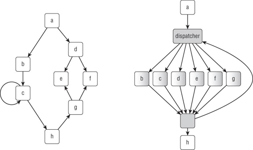
It goes without saying that a large part of this technique's resilience against static analysis rests on the ability to obfuscate the context's manipulations and transitions. Various features can be implemented to harden the problem, such as inter-procedural relationships, pointer aliasing, inserting dummy states, and so on.

In the same fashion as opaque predicates, CFG flattening can also be used to insert dead code paths and spurious basic blocks. A lot can be said about graph flattening and how to harden an implementation. The resulting graph offers no clues about the structure of the algorithm, and dispatch and context manipulation code also add an overhead that contributes to hiding the protected code. This technique is conceptually the same as code virtualization (virtual machine); it can be seen as partial virtualization that targets (virtualizes) only the control flow (not the data flow).

Should you want to see flattened code yourself, just grab a copy of a Flash plugin (such as NPSWF32.dll), disassemble the file, and look for functions with the biggest size. Flattened functions are easily recognizable.

Virtual Machines

Virtual machines (VMs) are a potent class of software protection and an especially complex transformation. A VM basically consists of an interpreter and some bytecode. The language supported by the interpreter is at the discretion of the protection. At compile-time, selected parts of code are compiled with respect to the VM's target architecture (they are retargeted) and then inserted into the protected program alongside the associated interpreter. At run-time, the interpreter assumes the bytecode execution (i.e., the translation from target architecture to original architecture). VMs usually come with sizeable overhead in terms of performance (particularly CPU time), which is why typically only specific, selected parts of the original program are virtualized.

Examples of well-known, VM-centered protections include VMProtect and CodeVirtualizer. We will later delve into the delightful activity of VM analysis. For now, suffice it to say that an attacker has to understand the interpreter in order to analyze the bytecode and eventually to create a compiler from target architecture to native architecture (unvirtualization).

White Box Cryptography

When the application to be protected cannot base its security on the use of a hardware component, or on a network server, you must hypothesize an attacker able to execute the application in an environment that he or she perfectly controls. The attacker model matching this situation, called thewhite-box attack context (WBAC), imposes a particular software implementation of classical cryptographic primitives.

Such mechanisms are tailor-made to ensure confidentiality of a secret key within an algorithm. Such a transformation (hiding a key in an encryption algorithm, with or without the help of environment interaction) can be formalized as an obfuscation transformation.

This section describes some negative and positive results concerning code obfuscation, and their impact on this key management problem.

A probabilistic algorithm O is an obfuscator if it satisfies the following properties, given by Barak et al.²:

· P and O(P) compute the same function.

· The growth of execution time and space of O(P) is at most polynomial in regard to execution time and space of program P.

· For any polynomial time probabilistic algorithm A, there exists a polynomial time probabilistic algorithm S and a negligible function m (a negligible function is a function that grows much slower than the inverse of any polynomial), such as the following: for all programs P,

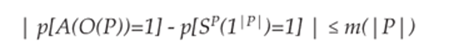
The virtual black box property expresses the fact that the outputs distribution of any probabilistic analysis algorithm A applied to the obfuscated program O(P) is almost everywhere equal to the outputs distribution of a simulator S making oracle access to program P. (Program S does not have access to the description of program P, but for any entry x, it is given access to P(x) in polynomial time in regard to the size of P. An oracle access to program P is equivalent to an access to sole inputs/outputs of the program P.)

Intuitively, the virtual black box property simply stipulates that everything that can be calculated from the obfuscated version O(P) can also be calculated via oracle access to P.

One of the main points about such an ideal obfuscator is that it does not exist. The proof is based on the construction of a program that cannot be obfuscated. This impossibility result demonstrates that a virtual black box generator—which could protect the code of any program by preventing it from revealing more information than is revealed by its inputs/outputs—does not exist. This impossibility result naturally leads to important outcomes for designers of obfuscation mechanisms (adapted to WBAC context).

Consider a practical application of obfuscation that consists of transforming a symmetric encryption into an asymmetric encryption, by obfuscating the private key encryption scheme. An unobfuscatable private key encryption scheme does exist if a private key encryption scheme exists. This clearly indicates that private key encryption schemes are not all well suited for obfuscation.

Note that this result does not prove that there is not some private key encryption scheme such that we can give to the attacker a circuit calculating the encryption algorithm without security loss. It does prove, however, that there is no general method enabling the transformation of any private key encryption scheme into a public key encryption system by obfuscating the encryption algorithm.

The problem of constructing a private key encryption scheme verifying the virtual black box property (thus resilient in the WBAC context) remains of interest for cryptography researchers, even if the impossibility result concerning a generic way to manage it may seem discouraging. White box DES and AES implementations proposals illustrate this interest.

Obfuscation by using a network of encoded lookup tables makes it possible to obtain from DES and AES algorithm versions that are more resilient in the white box attack context. However, effective cryptanalysis of DES (such as the one done by Goubin²⁴) and AES (by Billet⁵) white box implementations has established that the problem of constructing a private key encryption scheme verifying the virtual black box property remains unsolved.

The ideal model of an obfuscator able to transform any program into a virtual black box cannot be implemented. In particular, there is no general transformation that enables, starting from an encryption algorithm and a key, obtaining an obfuscated version of this algorithm that could be published without leaking information about the key it contains.

However, this formalism does not establish that it is impossible to hide a key in an algorithm in order to transform a private key algorithm into public key encryption.

A method has been published (by Chow⁹) to make the extraction of the key difficult in the white box context. The principle is to implement a specialized version of the DES algorithm that embeds the key K, and which is able to do only one of the two operations, encrypt or decrypt. This implementation is resilient in a white box context because it is difficult to extract the key K by observing the operations carried out by the program and because it is difficult to forge the decryption function starting from the implementation of the encryption function, and inversely.

The main idea is to express the algorithm as a sequence (or a network) of lookup tables, and to obfuscate these tables by encoding their input/output. All the operations of the block cipher, such as the addition modulo 2 of the round key, are embedded in these lookup tables. These tables are randomized, in order to obfuscate their functioning.

Obfuscation of AES (described by Chow¹⁰) is done in a similar way as DES. The goal is still to embed the round keys in algorithm code, in order to avoid storing the key in static memory or loading it in dynamic memory at the time of execution. The technique used to securely embed these keys is (as for DES) to represent AES as a network of lookup tables, and to apply input/output encodings in order to hide the keys.

Achieving Security by Obscurity

So far, you have seen a great number of obfuscation techniques. Most of them are simple transformations that seem quite weak at first sight—and they are actually weak considered individually. How one can build security or trust from such primitives? The strength of an obfuscation system (or obfuscator) comes from the iterative and combined applications of a set of these techniques. Each successive application of a simple technique accrues into a strong indiscernible global transformation (well, at least that is the objective). An interesting analogy has been proposed by Jakubowski et al.²⁶ between round-based cryptography and iterated obfuscation. A cryptographic algorithm's round is made of basic arithmetic operations (addition, exclusive or, etc.) that perform trivial transformations on the inputs. Considered individually, a round is weak and prone to multiple forms of attacks. Nevertheless, applying a set of rounds multiple times can result in a somewhat secure algorithm. That is the objective of an obfuscator. The objective of the attacker is to discern the rounds from the global obfuscated form and to attack them at their weakest points.

Keep in mind that even if the obfuscator is not perfect, as soon as it raises the bar required to break into the protected code by a sufficient amount, this may be sufficient for the defender. For example, if a few weeks or months are required to break into a new version of software, the defender can take advantage of that period to work on new protections, protocol updates, and so on, and thus always be ahead of the game.

A Survey of Deobfuscation Techniques

Now that you have a better understanding of code obfuscation, the question is how can you, as a reverse engineer, take up the challenge? What means and tools are at your disposal to break into obfuscated code? Manual analysis of obfuscated code is a tedious, if not impossible, task; you'll want to boil down the problem to clean code analysis.

Because a manual approach using standard program analysis tools is fastidious, and considering the wide variety of obfuscation mechanisms that an analyst may face, it is necessary to find some models and criteria to design and evaluate deobfuscation algorithms. This section provides a brief overview of the problem from a more theoretical perspective, and describes some well-studied formal methods that can be used to design more generic deobfuscation tools and automate as much as possible the tasks undertaken by an analyst.

The Nature of Deobfuscation: Transformation Inversion

In order to undo obfuscation transformation, several software analysis techniques are available. This section covers the following:

· The notion of decidable approximation

· Some methods, either static or dynamic, that can be used, and advantages that can be gained from hybrid static dynamic methods (some of them are presented later through the use of specialized tools)

· Some criteria that can always been applied to evaluate an analysis algorithm and from which it is possible to derive some security criteria about obfuscation robustness (and in a dual way a deobfuscation transformation efficiency)

· Open problems and new trends concerning hybrid dynamic/static analysis and formalization of deobfuscation

The subject is vast, and there is still no consensus about the terminology for the various specialized areas of research in the literature. The goal of this section is thus to provide readers with some keywords to enable a global view, and some useful references for interested readers who want to supplement their knowledge in this domain.

You can observe several dichotomies in the field of software analysis. Some analysis techniques are described as static or dynamic, even if this distinction sometimes seems quite artificial. (This distinction is discussed by Yannis Smaragdakis and Christoph Csallner³⁸.) Otherwise, analysis algorithms are qualified as sound or complete, but these important characteristics may have different meanings in the literature. Finally, program analyses are described as over-approximation or under-approximation, but this distinction also seems somewhat artificial because some analysis methods appear to use both over- and under-approximation.

The remainder of this section discusses both the “synergy” and “duality” of static and dynamic analysis (also discussed by Michael D. Ernst²⁰), first introducing the formal model of abstract interpretation and then providing several analysis examples in relation to deobfuscation.

Finding a Decidable Approximation of the Concrete Semantics

The purpose of any program analysis is to check whether the program satisfies a certain property. Unfortunately, the question is generally undecidable for any non-trivial property—that is to say, you cannot design an algorithm to determine whether the property holds for the program. To overcome this difficulty, one solution is to abstract the concrete behaviors of the program into a decidable approximation. The purpose of abstract interpretation is to formalize this idea of approximation in a unified framework. (Readers can refer to the paper by Patrick Cousot and Radia Cousot.¹⁴)

The semantics of a program represent all of its possible concrete behavior, including its interaction with any possible computer system environment. Among the most precise (concrete) semantics are the so-called trace semantics. This semantics includes all finite and infinite sequences of states and transitions. Where X is the set of execution traces (finite and infinite), you can express the trace semantics as the least solution (for the computational partial ordering) of a fixpoint equation X=F(X).

An abstract domain is an abstraction of a concrete semantics. The goal of abstract interpretation is to provide computable, fixpoint approximations of abstract domains, thus defining computable abstract semantics. Obviously, the coarser the abstract semantics, the fewer questions it can answer.

All abstractions of a semantics can be organized in a hierarchy (described by Cousot¹⁶), from the most precise to the coarsest. More precisely, abstract semantics can be placed on a lattice, and the approximation partial ordering of this lattice can be used to characterize the concreteness (or precision) of abstract semantics, and thus the sets of questions they are able to answer.

Abstract interpretation generally applies to static analysis, through an over-approximation of the concrete semantics. You might notice that, in a dual way and according to the “dual principle” of lattice theory, it should also apply to dynamic analysis, even if there are not currently many works on this subject. You will see in the next section that relations and synergy between static and dynamic analysis lead to practical hybrid dynamic/static methods, making it possible both for a dynamic approach to gain in coverage and for a static approach to gain in precision.

Dynamic and Static Analyses Form a Continuum

Static analysis is the discipline of automatically inferring information about computer programs without running them (it thus applies to a “static” representation of the program). Static analysis tries to derive properties (invariants) that hold for all executions of the program, through a conservative over-approximation of its concrete semantics.

An example of such static analysis is the constant propagation algorithm, which aims to determine for each program instruction whether a variable has a constant value whenever the control flow reaches that instruction. Information about constants is useful in the context of program compilation, optimization, and recompilation. It is used, for example, for dead code and dead execution path deletion (by replacing all uses of constant variables by their constant values, you may be able to identify constant conditional branches, which are conditioned by constant predicates).

Among the many optimization techniques, partial evaluation techniques (described by Beckman et al.³) must be kept in mind in the context of reverse engineering. A partial evaluator specializes a program with regard to part of its input data. You expect the program's concrete semantics to be preserved by the specialization process and the resulting program's syntactic representation to be optimized for the class of inputs used, and as a result simpler to understand.

Another important class of optimization techniques includes slicing techniques (described by Weiser⁴²), which also aim to simplify the program under consideration, but in this case by deleting those parts of the program that are irrelevant according to a criterion provided by the analyst. A static slicing criterion includes a set of variables and a chosen point of interest. A dynamic slicing criterion completes a static criterion with the information corresponding to some concrete execution. Slicing is of great interest in the reverse engineering context, because it is representative of the way a reverser mentally slices a program when attempting to understand its inner working.

In contrast to static analysis, dynamic analysis is the discipline of automatically inferring information about a running computer program. Dynamic analysis derives properties that hold for one or more executions of a program, through a precise under-approximation.

A common method of dynamic analysis is dynamic testing, which executes a program with several inputs and checks the program's response. Generally, test cases explore only a subset of the possible executions of the program.

In order to enlarge the coverage of dynamic testing, the principle of symbolic execution (described by Boyer⁶) uses symbolic values rather than concrete inputs. At any point during symbolic execution, a symbolic state of the program is updated. This symbolic state consists of a symbolic storeand a path constraint. The symbolic store contains the symbolic values, and the path constraint is a formula that records the history of all conditional branches taken until the current instruction.

At a given instruction of the program, you can use a constraint solver (SMT or SAT solver) to determine the corresponding path constraint. A satisfying assignment provides concrete inputs with which the program reaches the program instruction. By generating new tests and exploring new paths, you can increase the coverage of dynamic testing.

Unfortunately, constraints generated during symbolic execution may be too complex for the constraint solver. If the constraint solver is unable to compute a satisfying assignment, you cannot determine whether a path is feasible or not.

Concolic execution (described by Godefroid²³ and Sen³⁷) provides a solution to this problem in many situations. The idea is to perform both symbolic execution and concrete execution of a program. When the path constraint is too complex for the constraint solver, you can use the concrete information to simplify the constraint (typically by replacing some of the symbolic values with concrete values). You can then expect to find a satisfying assignment of this simplified constraint.

Because symbolic execution is unable to handle an unbounded loop, which results in infinite symbolic execution paths, it must under-approximate the concrete semantics of the program. You can perform this simplification by fixing some arbitrary loop limit. Another solution is to use symbolic execution in conjunction with a static analysis inferring loop invariants.

It appears that dynamic and static analysis approaches form a continuum. As an illustration, dynamic testing, symbolic execution, and abstract interpretation are three ways of approximating the concrete semantics of a program. Dynamic analysis uses concrete values and explores a subset of concrete transitions. Symbolic execution clearly lies between dynamic testing and static analysis. It rests on a more abstract semantics, but also an under-approximation. An abstract interpreter over-approximates the concrete semantics of the program.

However, the borderline between those analysis approaches is not so easy to define. For example, symbolic execution can be defined as a logical abstract interpreter, operating over the abstract domain of logical formulas.

In conclusion, many static analysis methods are improved by the use of a dynamic analysis–based refinement. Conversely, the coverage of many dynamic analysis methods can be increased by using traditional static analysis methods. Thus, the investigation of hybrid dynamic/static approaches is of great interest, especially in the context of reverse engineering. The soundness and completeness criteria can be used to capture this synergy.

Soundness and Completeness

You can formulate any program analysis problem as verification that the program satisfies a property. Two fundamental concepts can be used to characterize an analysis algorithm: its soundness and its completeness. These concepts, traditionally applied to logical systems, can also be applied to program analysis. Unfortunately, because of their dual natures (soundness and completeness correspond to converse implications in logic), there is still no consensus regarding their application to the various specialized areas of research in the literature.

Given a property, a sound program analysis identifies all violations of the property. However, because it over-approximates the behaviors of the program, it may also report violations of the property that cannot occur. For example, a sound error detection algorithm detects every possible error, though some of them may not occur at run-time.

A sound partial evaluation algorithm preserves the original program's concrete semantics, in the sense that the specialized program does not produce any output value that is not produced by the original program (even if it may not be able to produce all of them).

A sound symbolic execution guarantees that because a symbolic constraint path is satisfiable, there must be a concrete execution path that reaches the corresponding concrete state (even if some reachable concrete state does not have a corresponding symbolic state).

A sound abstract interpreter preserves the program's concrete semantics. If it claims that an optimization transformation is possible for a program, then the optimization can be applied without breaking the program semantics. Observe, however, that it may be unable to answer the question for some optimizations. It can claim that an optimization is unsafe even if it is in fact possible to apply the transformation (without any destructive effect). Some potential optimizations will not be applied. The soundness of the abstract interpreter is relative to which questions it can answer correctly, despite the loss of information. In that sense, it is conservative. Technically, the least fixpoints computed by an abstract interpreter represent at least all occurring run-time concrete states.

For example, a constant propagation algorithm is sound when any constant it detects is indeed a constant. However, some constants may be not detected. Given a property, a complete analysis algorithm reports a violation of the property only if there is a concrete violation of the property. However, because it under-approximates the behaviors of the program, some concrete violations of the property may not be reported.

A complete partial evaluation algorithm results in the generation of a specialized program that is able to produce the same output values as the original program for the intended input values. If unsound, it may produce unexpected output values (i.e., not produced by the original program).

A complete symbolic execution covers all concrete transitions. It guarantees that if a concrete execution state is reachable, then there must be a corresponding symbolic state. Because symbolic execution is unable to handle an unbounded loop, which results in infinite symbolic execution paths, it must under-approximate the concrete semantics of the program (typically by providing some loop limit). Therefore, symbolic execution algorithms are most often incomplete.

A complete abstract interpreter is the most precise for answering a given set of questions. Technically, this means that every state represented by the least fixpoint is reachable for some concrete input. For example, a complete constant propagation algorithm would be able to detect every constant in a program.

We have presented some criteria (soundness and completeness) that can always be applied to evaluate an analysis algorithm. It is possible to derive from them some security criteria about obfuscation robustness (and, in a dual way, deobfuscation transformation efficiency).

Abstract interpretation can be used for modeling any program transformation (refer to the paper by Patrick and Radia Cousot¹⁵). By considering the syntax of a program as an abstraction of its concrete semantics, we can formalize any syntactic program transformation as an abstract interpretation of the corresponding semantic transformation.

A particular application of this concerns obfuscation and deobfuscation transformations modeling. Mila Dalla Preda and Roberto Giacobazzi¹⁸ investigate the semantic transformations corresponding to opaque predicate insertion. By modeling deobfuscation as an abstraction interpretation, they observe that breaking opaque predicates corresponds to having complete abstraction. The completeness criterion turns out to be of special interest in terms of qualifying both deobfuscator effectiveness and opaque predicate robustness.

In conclusion, many methods already used in program analysis and compilation are of interest in the context of reverse engineering. As demonstrated earlier, the frontier between static and dynamic analysis is not so obvious. Currently, the abstract interpretation model seems to be sufficiently general to apply to both types of analyses. The soundness and completeness criteria are of special interest when modeling obfuscation and deobfuscation transformations in the abstract interpretation framework. You have seen that both the soundness and the completeness of an algorithm can be defined for static and dynamic analyses (data flow analyses, partial evaluation, slicing, symbolic execution), which are good candidates to represent the actions conducted by reversers when they try to simplify the representation of an obfuscated program. Using the abstract interpretation model, static and dynamic analyses appear to be dual in nature. This duality and the gain that can be obtained from a synergy between static and dynamic methods lead to new possibilities that must be investigated in the future, through the study of hybrid methods.

This section presented some academic models and criteria, as well as dynamic and static analysis methods, that can be useful for designing and evaluating deobfuscation algorithms. It also stressed the importance of hybrid methods. The next section presents some of the tools currently available to assist in undoing obfuscation transformations.

Deobfuscation Tools

In this section we discuss some of the tools that you can use to reverse engineer obfuscated code and especially the features they offer to ease your job. Please note that this list is not meant to be exhaustive in any way; it is based on the experience of some of the authors and seeks to present different categories of tools.

IDA

IDA is the state-of-the-art tool for reverse engineering binary code. Throwing the binary one wants to analyze into IDA is a common reflex, so there's probably no need to introduce this tool here; otherwise, readers can refer to the The IDA Pro Book by Chris Eagle (No Starch Press, 2011). Regarding the specific topic that interests us here, dealing with obfuscated code using IDA is problematic (although not impossible) for a few reasons:

· That's not the purpose for which IDA is primarily intended. Obfuscated code is a very particular case, and handling every specific situation/trick would be an endless job; thus it's better not to start on this path.

· We have very little control over the disassembler, a point that greatly impedes us when encountering obfuscation schemes that break/disrupt/destroy the control-flow graph. IDA's disassembler is really easy to confuse and one often ends up with the chicken-and-egg problem: To recover the control flow one needs to clean the data flow, but to clean the data flow one needs the control flow.

· IDA itself doesn't offer any sort of intermediate representation (IR) or at least instruction semantics, so advanced analysis of its output is not trivial.

In 2008 at the ICAR workshop (http://www.hex-rays.com/ products/ida/support/ppt/caro_obfuscation.ppt), Ilfak Guilfanov offered some useful tips on how to use specific features of IDA:

· Graph-level block merging to simplify the CFG

· Event-driven, on-the-fly modification of the graph using hooks like grcode_changed_graph (see graph.hpp in the SDK)

· Develop specific plugins

IDA can be extended using scripts (either IDC or IDAPython) or plugins (see IDA's SDK). If you were to implement some advanced analysis, that's where you would be able to interact.

To that end, some plugins have been developed as deobfuscation frameworks (for example, Branko Spasojevic's Optimice plugin, http://optimice.googlecode.com). Trying to address some of the issues previously mentioned, including instruction semantics—based on the x86 Opcode and Instruction Reference (http://ref.x86asm.net/)—the plugin offers CFG reduction, peephole optimizations, and dead code removal.

Metasm

Metasm (http://metasm.cr0.org) is open source framework (released under the GNU Lesser GPL v2) developed by Yoann Guillot. It defines itself as an assembly manipulation suite. The framework, written in Ruby, actually offers cross-architecture assembler, disassembler, compiler, linker, and debugger features. Currently supported processors are Intel x86/x64, MIPS, PPC, Sh4, and ARCompact. Most common file formats are supported as well, such as MZ, PE/COFF, ELF, Mach-O, and so on.

Disassembler Callbacks

The behavior of the disassemblery can be dynamically modified using a set of exported callbacks of the Disassembler class. The two most useful for deobfuscation are as follows:

· callback_newaddr—This is called each time a path is discovered and is about to be disassembled. At this point you can inspect the path backward or forward for unseemliness; most important, you can modify the behavior of the disassembly engine—removing a spurious control transfer, thwarting a disassembler trap, etc.

· callback_newinstr—As its name suggests, your callback is called each time a new instruction is disassembled.

Instruction Semantics

One of the framework's key features is backtracking (think of it as program slicing). This feature is at the heart of its disassembly engine. It enables very precise control flow recovery, at the cost of performance. Built on top of this feature, the framework's API also offers a method to compute the semantics of a basic block. Metasm does not use a strict intermediate language, however; it relies on a description of the semantics of each instruction. The associated terminology in the framework is binding. Metasm separates control flow and data flow semantics encoding. Four types are used to describe the semantics of an instruction:

· Numerical value

· Symbol—Whatever is not a numerical value, based on Ruby's symbol type

· Expression: Expression[operand1, (operator), (operand2)]—An operand can be any of the four types.

· Indirection—Memory indirection Indirection[target, size, origin]

The following snippet will introduce you to the Metasm instructions' binding:

# encoding: ASCII-8BIT

#!/usr/bin/env ruby

require "metasm"

include Metasm

# produce x86 code

sc = Metasm::Shellcode.assemble(Metasm::Ia32.new, EOS)

add eax, 0x1234

mov [eax], 0x1234

ret

EOS

dasm = sc.init_disassembler

# disassemble handler code

dasm.disassemble(0)

# get decoded instruction at address 0

# then its basic block

bb = dasm.di_at(0).block

# display disassembled code

puts "\n[+] generated code:"

puts bb.list

# run though the basic block's list of decoded instruction

bb.list.each{|di|

puts "\n[+] #{di.instruction}"

sem = di.backtrace_binding()

puts " data flow:"

sem.each{|key, value| puts * #{key} => #{value}"}

# does instruction modify the instruction pointer ?

if di.opcode.props[:setip]

puts " control flow:"

# then display control flow semantics

puts " * #{dasm.get_xrefs_x(di)}"

end

}

For each DecodedInstruction, you call the backtrace_binding method. It returns a hash. Each key/value pair represents an assignment of the key according to the value and expresses outputs with respect to inputs. Running the scripts produces the following result:

[+] generated code:

0 add eax, 1234h

5 mov dword ptr [eax], 1234h

0bh ret ; endsub entrypoint_0

[+] add eax, 1234h

data flow:

* eax => eax+1234h

* eflag_z => ((eax+1234h)&0ffffffffh)==0

* eflag_s => (((eax+1234h)1fh)&1)!=0

* eflag_c => ((eax&0ffffffffh)+1234h)>0ffffffffh

* eflag_o => (((eax1fh)&1)==0)&&((((eax1fh)&1)!=0)!=

((((eax+1234h)1fh)&1)!=0))

[+] mov dword ptr [eax], 1234h

data flow:

* dword ptr [eax] => 4660

[+] ret

data flow:

* esp => esp+4+0

control flow:

* [Indirection[Expression[:esp], 4, 0xb]]

The RET instruction is quite representative of the distinction between data flow and control flow. The get_xrefs_x method provided by the disassembler object returns a list (a Ruby Array object) of possible values for the instruction pointer. For that specific instruction, it is an indirection whose target is the ESP register and whose size is 4 (for the Ia32 architecture)—i.e., dword ptr [ESP]; 0xb is the address in the program where the indirection occurs.

Backtracking and Slicing

So far, you have seen how the semantics are described for each isolated instruction. Now consider instructions within a control flow and how an instruction's binding can be used. For this purpose, the following example demonstrates a typical dynamic jump computation pattern:

# encoding: ASCII-8BIT

#!/usr/bin/env ruby

require "metasm"

include Metasm

# produce handler's x86 code

sc = Metasm::Shellcode.assemble(Metasm::Ia32.new, EOS)

entry:

mov ecx, 1

shl ecx, 0xA

add edx, 0xBADC0FFE

mov eax, 0x100000

lea eax, [ecx+eax]

add ecx, 0xBADC0FFE

jmp eax

EOS

# disassemble handler code

dasm = sc.init_disassembler

dasm.disassemble(0)

# get basic block

bb = dasm.block_at(0)

target = dasm.get_xrefs_x(bb.list.last).first

puts "[+] jmp target: #{target}"

# backtrace

values = dasm.backtrace(target, bb.list.last.address,

{:log => bt_log = [], :include_start => true})

get_xrefs_x tells you which target is the final jump instruction. Then the backtrace method is used to walk back through the control flow, following variable dependencies, until it reaches variable assignations or simply hits its complexity limit. Each step of the backtracker is stored within the array bt_log. The following adds a few more lines to nicely output the record:

bt_log.each{|entry|

case type = entry.first

when :start

entry, expr, addr = entry

puts "[start] backtacking expr #{expr} from 0x#{addr.to_s(16)}"

when :di

entry, to, from, instr = entry

puts "[update] instr #{instr},\n -> update expr from #{from} to

#{to}\n"

when :found

entry, final = entry

puts "[found] possible value: #{final.first}\n"

when :up

entry, to, from, addr_down, addr_up = entry

puts "[up] addr 0x#{addr_down.to_s(16)} -> 0x#{addr_up.to_s(16)}"

end

}

Here is the output from the sample:

[+] jmp target: eax

[start] backtacking expr eax from 0x1c

[update] instr 13h lea eax, [ecx+eax],

-> update expr from eax to ecx+eax

[update] instr 0eh mov eax, 100000h,

-> update expr from ecx+eax to ecx+100000h

[update] instr 5 shl ecx, 0ah,

-> update expr from ecx+100000h to (ecx0ah)+100000h

[update] instr 0 mov ecx, 1,

-> update expr from (ecx0ah)+100000h to 100400h

[found] possible value: 100400h

The backtracking engine has been able to walk back the instruction flow to compute the final value of the backtracked expression. A simplification engine enables solving (or at least reducing) expressions at both the symbolic and numerical levels.

From the log record it is even possible to extract a slice—that is, the minimal subset of the original program that produces the studied effect (the slicing criterion). In this case the slice will contain all the instructions involved in the computation of the JMP destination:

# DecodedInstruction object is the 3rd item of :id entry

slice = bt_log.select{|e| e.first==:di}.map{|e| e[3]}.reverse

puts slice

The slice is as follows:

0 mov ecx, 1

5 shl ecx, 0ah

0eh mov eax, 100000h

13h lea eax, [ecx+eax]

Note how nonsignificant computations/assignations (e.g., the ones using the constant 0BADC0FFEh) have been eliminated from this list.

That sample is an ideal case: The expression can statically be reduced/solved into a numerical value. Now, imagine you remove the first assembly line (MOV ECX, 1)—within the basic block scope ECX is undefined—and then redo the analysis:

[+] jmp target: eax

[start] backtacking expr eax from 0x17

[update] instr 0eh lea eax, [ecx+eax],

-> update expr from eax to ecx+eax

[update] instr 9 mov eax, 100000h,

-> update expr from ecx+eax to ecx+100000h

[update] instr 0 shl ecx, 0ah,

-> update expr from ecx+100000h to (ecx0ah)+100000h

The return value is an object of type Expression whose value is (ECX0Ah)+100000h.

This example is fairly trivial. The capacity of the backtracker goes far beyond that. The following modifies the preceding sample to include a more complex control-flow graph:

# produce handler's x86 code

sc = Metasm::Shellcode.assemble(Metasm::Ia32.new, EOS)

entry:

mov ecx, 1

test edx, edx

jnz label inc cl

label:

shl ecx, 0xA

add edx, 0xBADC0FFE

mov eax, 0x100000

lea eax, [ecx+eax]

add ecx, 0xBADC0FFE

jmp eax

EOS

# disassemble handler code

dasm = sc.init_disassembler

dasm.disassemble(0)

# get last basic block

bblist = dasm.instructionblocks.sort{|b1, b2| b1.address <=> b2.address}

bblist.each{|bb| puts "-\n", bb.list}

bb = bblist.last

Basically, this has inserted an instruction (TEST EDX, EDX) controlling a conditional jump; in one case ECX is incremented, in the other it is not. The updated output is as follows:

[+] jmp target: eax

[start] backtacking expr eax from 0x21

[update] instr 18h lea eax, [ecx+eax],

-> update expr from eax to ecx+eax

[update] instr 13h mov eax, 100000h,

-> update expr from ecx+eax to ecx+100000h

[update] instr 0ah shl ecx, 0ah,

-> update expr from ecx+100000h to (ecx0ah)+100000h

[up] addr 0xa -> 0x9

[up] addr 0xa -> 0x7

[update] instr 0 mov ecx, 1,

-> update expr from (ecx0ah)+100000h to 100400h

[found] possible value: 100400h

[update] instr 9 inc ecx,

-> update expr from (ecx0ah)+100000h to ((ecx+1)0ah)+100000h

[up] addr 0x9 -> 0x7

[update] instr 0 mov ecx, 1,

-> update expr from ((ecx+1)0ah)+100000h to 100800h

[found] possible value: 100800h

The backtracker returns an array of two possible values: 100400h or 100800h. Note how it has followed the control flow over the CFG. (Both branches of the conditional have been followed.) An [up] tag indicates a basic block's crossing. Backtracking really is at the heart of the disassembler and produces a more accurate disassembly. Obviously, this feature comes with severe performance penalties (remember the trade-off between computability and precision).

Code Binding

You know how to obtain the semantics of an isolated instruction, and you know how to backtrack a value and compute a slice for that particular value. What if you could generalize this process and compute the semantics of a basic block? This is another very powerful feature of Metasm: thecode_binding method, provided by the disassembler object. It totally relies on the backtracking feature. Here is its usage on the last basic block of the previous example:

# compute basic block's semantics

bbsem = dasm.code_binding(bb.list.first.address, bb.list.last.address)

puts "\n[+] basic block semantics"

bbsem.each{|key, value| puts " * #{key} => #{value}"}

Its output is as follows:

[+] basic block semantics

* eax => ((ecx0ah)+100000h)

* ecx => ((ecx0ah)+badc0ffeh)

* edx => (edx+badc0ffeh)

Miasm

Miasm (http://code.google.com/p/smiasm) is a reverse engineering framework developed by Fabrice Desclaux that offers PE/ELF manipulation, assembling, and disassembling (currently supports Ia32, ARM, PPC, and Java bytecode). Like Metasm, Miasm is open source and released under the GNU Lesser GPL v2, so you can delve into its engine to customize specific needs. The examples provided in this section are based on the latest revision of MIASM available at the time of writing (changeset:270:6ee8e9a58648).

The framework relies on an intermediate language. That means most common instructions have their semantics encoded as a list of expressions. “List” is to be understood in its Python meaning (i.e., an ordered set of objects). The grammar of Miasm's IR makes use of nine basic expression types, the most important of which are as follows:

· ExprInt—Numerical value

· ExprId—Identifier/symbol, whatever is not a numerical value; for example, registers are defined as ExprId

· ExprAff—Affectation a = b

· ExprCond—Ternary/conditional operator a ? b : c

· ExprMem—Memory indirection

· ExprOp—Operation op(a,b,…)

It also provides full support for slices (think of it as an object to represent bitfields) and slice composition. The IR allows symbolic computations and is equipped with an expression simplification engine.

For each supported processor, a “sem” suffixed file describes the semantics of most common instructions. See, for example, the ADD semantics as defined in “miasm/arch/ia32 sem.py”:

def add(info, a, b):

e= []

c = ExprOp('+', a, b)

e+=update_flag_arith(c)

e+=update_flag_af(c)

e+=update_flag_add(a, b, c)

e.append(ExprAff(a, c))

return e

This function builds the semantics of the instructions based on its two operands (a and b). One can easily write a piece of script to demonstrate these features:

#! /usr/bin/env python

from miasm.arch.ia32_arch import *

from miasm.tools.emul_helper import *

# assemble instruction asm at given address

def instr_sem(instr, address):

print "\n[+] instruction %s @ 0x%x" % (instr, address)

binary = x86_mn.asm(instr)

di = x86_mn.dis(binary[0])

semantics = get_instr_expr(di, address)

for expr in semantics:

print " %s" % expr

instr_sem("add eax, 0x1234", 0)

instr_sem("mov [eax], 0x1234", 0)

instr_sem("ret", 0)

instr_sem("je 0x1000", 0)

Here is the output:

[+] instruction add eax, 0x1234 @ 0x0

zf = ((eax + 0x1234) == 0x0)

nf = ((0x1 == ((eax + 0x1234) 0x1F)) & 0x1)

pf = (parity (eax + 0x1234)) af = (((eax + 0x1234) & 0x10) == 0x10)

cf = ((0x1 == (((eax ^ 0x1234) ^ (eax + 0x1234)) 0x1F)) ^

(0x1 == ((((eax + 0x1234)) & (! (eax ^ 0x1234))) 0x1F)))

of = (0x1 == (((eax ^ (eax + 0x1234)) & (! (eax ^ 0x1234))) 0x1F))

eax = (eax + 0x1234)

[+] instruction mov [eax], 0x1234 @ 0x0

@32[eax] = 0x1234

[+] instruction ret @ 0x0

esp = (esp + (0x4 + 0x0))

eip = @32[esp]

[+] instruction je 0x1000 @ 0x0

eip = (zf == 0x1)?(0x1000,0)

The ADD instruction's semantics seem the most complex, due to the flags update. Here is the MOV instruction's semantics with an explicit typing of object:

[+] instruction mov [eax], 0x1234 @ 0x0

ExprAff( ExprMem(@32[ExprId(eax)]) = ExprInt(0x1234) )

This is a very appreciable and powerful feature. Built upon the IR, there is a just-in-time (JIT) compilation feature whereby code is first disassembled, translated into IR, then regenerated as native code for execution. The documentation and samples provide use cases of Miasm for packer/VM analysis as well as binary instrumentation.

VxStripper

VxStripper is a binary rewriting tool, developed by Sébastien Josse. Designed for analysis of protected and potentially hostile binary programs, it dynamically extracts an intermediate representation of a binary executable and all the necessary information to apply certain simplifications, making the binary inner workings easier to understand for the analyst.

One of the main motivations behind the design and implementation options of this tool is to circumvent current limitations of existing malware and binary programs analysis solutions. (Many tools come with their own intermediate representation—non-exportable, sometimes proprietary—making difficult their integration. Moreover, many of them are not suitable for analysis of hostile or protected code.) The goal is to get as much information as possible from a binary program that uses all available techniques and tools to protect this information. The idea is to instrument a virtual computer processing unit and a guest operating system in a non-intrusive way to dynamically get information required to rebuild the program and simplify its representation. This tool is based on the dynamic binary translator engine of QEMU and on the LLVM compilation chain.

LLVM (Low Level Virtual Machine) is a compilation chain that comes with a consequent set of optimizations that can be applied across the entire lifetime of a program. LLVM uses a strongly typed RISC-like instruction set and a static single assignment (SSA) representation (using this representation, each temporary variable is assigned only once). LLVM includes many binary back-ends (x86, x86-64, SPARC, PowerPC, ARM, MIPS, CellSPU, XCore, MSP430, MicroBlaze, PTX) and some source code back-ends (C, C++). Readers can refer to the paper by Lattner³¹ for further details about LLVM.

The QEMU (Quick EMUlator) Dynamic Binary Translator (DBT) is used to dynamically translate the binary code from the guest CPU architecture to the host CPU architecture, through the use of an IR called TCG (Tiny Code Generator). This language consists of simple RISC-like instructions called micro-operations. The binary translation consists of two stages. The guest binary code is first translated in sequences of TCG instructions, called translation blocks (DBT front end). Then, the translation blocks are converted into code executable by the host CPU (DBT back end). QEMU's DBT comes with many binary front ends (x86, x86-64, ARM, ETRAX CRIS, MIPS, Micro Blaze, PowerPC, SH4, and SPARC). Readers can refer to the paper from Bellard⁴ for further details about QEMU.

VxStripper inherits from QEMU the many binary front ends, and from LLVM the many back ends, providing at reasonable cost a complete binary rewriting framework. The rewriting functions are implemented as LLVM passes.

Its current design builds upon work already done to convert TCG IR to LLVM IR (LLVM-QEMU, described by Scheller³⁶, and S2E, described by Chipounov⁸), as well as upon design algorithms presented by Josse.²⁷, ²⁸

One of the goals of this tool is collaboration with the many software analysis tools based on the LLVM compilation chain, through an “exported” representation of the malware program. This binary analysis tool is especially designed to solve the problem of hostile programs analysis. The goal is to automate the often fastidious and repetitive tasks driven by an analyst.

This compilation chain is based on a modular and evolutionary architecture, making it possible to apply the same transformations to a wide variety of software and hardware architectures. It is based on a modern compilation chain, providing efficient intermediate representation and functionalities.

Vellvm (Verified LLVM), described by Zhao,⁴³ provides formal tools to reason on transformations that operate on LLVM's intermediate representation. Vellvm can be used to extract formally verified implementations of deobfuscation passes implemented in VxStripper.

QEMU DBT Extension

You have seen that the QEMU DBT engine performs the dynamic translation of the binary code from the guest processor architecture to the host processor architecture by using the TCG intermediate representation.

Using a simple example, the following instruction demonstrates what this language looks like:

0x0040104c: push 0xa

The preceding instruction is translated as follows in the QEMU TCG representation:

(1) movi_i32 tmp0,$0xa

(2) mov_i32 tmp2,esp

(3) movi_i32 tmp13,$0xfffffffc

(4) add_i32 tmp2,tmp2,tmp13

(5) qemu_st32 tmp0,tmp2,$0x1

(6) mov_i32 esp,tmp2

(7) movi_i32 tmp4,$0x40104e

(8) st_i32 tmp4,env,$0x30

(9) exit_tb $0x0

This TCG instructions block emulates the execution of the push instruction on the software CPU. The performed operations are as follows: The integer 0xa is stored in the variable tmp0 (line 1). This variable is then stored on the stack (lines 2–6). The address of the instruction following the current instruction is stored in tmp4 (line 7) and then stored in the QEMU VPU register cc_op. The last instruction (line 9) indicates the end of the TCG block.

The tool modifies the DBT mechanism in such a way that the instrumentation function of the virtual CPU is systematically invoked before the execution of a translation block. To achieve this, you add an extra micro operation (op_callback) that takes as operand the address of the instrumentation function (vpu_callback).

The resulting TCG code is as follows:

(1) op_callback @vpu_callback

(2 movi_i32 tmp0,$0xa

(3) mov_i32 tmp2,esp

(4) movi_i32 tmp13,$0xfffffffc

(5) add_i32 tmp2,tmp2,tmp13

(6) qemu_st32 tmp0,tmp2,$0x1

(7) mov_i32 esp,tmp2

(8) movi_i32 tmp4,$0x40104e

(9) st_i32 tmp4,env,$0x30

(10) exit_tb $0x0

This mechanism enables you to execute your instrumentation code at each execution cycle of the virtual CPU. With access to VPU registers and to the virtual PC memory, you can acquire a process context and extract information about its interactions with the guest operating system.

By also instrumenting the load and storing TCG instructions, you can extract information about the interactions of the target process with the memory of the guest system. Thanks to this information, you can recover the relocation information of the process.

Now that you have seen how to modify the QEMU virtual CPU to enable the systematic invocation of your instrumentation function, let's examine the translation of TCG intermediate representation to LLVM representation. The result of translating the preceding TCG block is as follows:

(1) %esp_v.i = load i32* @esp_ptr

(2) %tmp2_v.i = add i32 %esp_v.i, -4

(3) %4 = inttoptr i32 %tmp2_v.i to i32*

(4) store i32 10, i32* %4

(5) store i32 %tmp2_v.i, i32* @esp_ptr

(6) store i32 4198478, i32* %next.i

(7) store i32 0, i32* %ret.i

The integer 0xa is stored at the address pointed to by the variable %4, which is equivalent to storing it on the stack (lines 1–4). The address of the instruction following the current instruction is stored in the variable %next.i (line 6). The last instruction (line 7) finishes the LLVM block.

After the normalization process, this LLVM block is compiled to the following assembly code:

401269! mov dword ptr [esp-14h], 0ah

Now that you have an overview of the main modifications applied to the QEMU emulator, as shown schematically in Figure 5.2, the following section describes the general architecture of the tool.

Figure 5.2

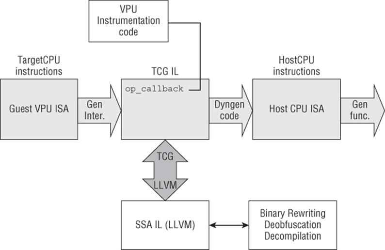
Architecture of VxStripper

VxStripper implements an extended DBT engine and several specialized analysis functions (see Figure 5.3) to observe the target program and its execution environment.

Figure 5.3

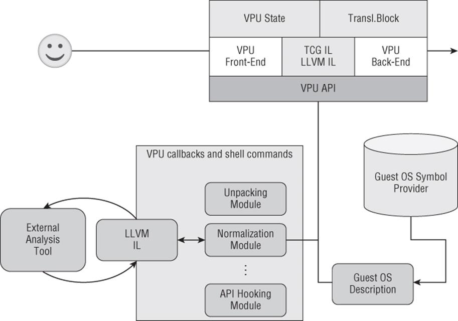
A module manager handles activation and collaboration between these analysis functions, implemented as plugins.

These analysis functions extract semantic information from the target program. This information can be the trace of its interactions with APIs of the guest operating system, or the way it handles objects and structures of the guest operating system's executive or kernel, or more simply its machine code trace.

The extraction of this information rests on a description of the guest operating system, which can be provided, for example, by a symbol server, as is the case for the family of Windows operating systems.

Among the modules already implemented, you notably find the following:

· An API hooking module

· A forensics analysis module

· An unpacking module

· A normalization module

API Hooking

The native and Windows API hooking module of VxStripper is based on forensic analysis of the guest operating system's memory, without any interaction with the guest operating system.

The Windows executive maintains a set of structures that contains information about the loaded modules for a given process inside its memory space. These data structures can be recovered by using the process environment block (PEB), which can itself be accessed as an offset of segment register FS. The native and Windows API hooking modules of VxStripper use this information to locate and instrument Windows API.

Forensics/Root-Kit Analysis

The forensics module of VxStripper comes with additional features to monitor and check the integrity of many locations within the guest platform where a hook can be installed. It walks through executive structures of the operating system in order to identify potential targets of a root-kit attack and monitor hardware components that could be corrupted by a root-kit. This information is crucial for the analyst to understand low-level viral attacks.

For the purposes of this chapter, you can consider these features to be similar to those expected from a kernel debugger. You can attach a process, view its CPU state and disassembled code, and trace the interaction of the target program with the operating system API. This inspection is done in a safe and controlled environment, without any intrusive interaction with the guest operating system.

The following two sections take a closer look at the working of Vxstripper's two most important analysis modules: the unpacking module and the normalization module.

Unpacking Module

The unpacking module locates the original entry point (OEP) of the target executable, gets information relative to its interactions with the operating system API, and extracts the relocation information.

The underlying idea is a simple integrity check of the target program's executable code: For each translation block of the program, a comparison between its value in virtual memory and its value on the host file system is made. As long as the values are identical, nothing is done. As soon as a difference is identified, the current translation block is written into the raw file in place of the old translation block. The first instruction of the newly generated translation block is identified as the OEP of the protected program. At the end of the analysis, data sections are written into the raw file in place of original data sections.

The same monitoring algorithm is applied for each translation block. The protection loader of the packed executable can have several deciphering layers. As soon as the last deciphered translation block has been reached, the only thing to be done is to repair the target executable. In order to recover the PE (Portable Executable) structure of an unprotected executable, several tasks have to be carried out: Set the original entry point, rebuild the imports and relocations tables, and consistency check the PE header.

The method used by the unpacking engine in order to reconstruct the Import Address Table (IAT) and relocations is based on Win32 and native API hooking. During the unpacking process, all API calls are traced. A sorted table of API calls is initialized at load-time, by walking NT executive structures.

Next, after process execution has resumed, each API call is traced. This table is updated regularly during the target process execution, and is used to dynamically resolve API function names. Finally, after a dump of the target process memory space is completed, this table is used to fix the IAT in the PE executable.

Thanks to the load and store TCG instructions instrumentation, you can dynamically extract the program's relocation information, which can also be added to a new section of the executable.

For example, here is the (useful) information extracted during the unpacking stage of a program that displays a dialog box (function MessageBoxA):

[INFO] eip=0x00401000

[RELOC] value=0x00403000 va=0x00401003

[RELOC] value=0x0040300f va=0x00401008

[RELOC] value=0x00402008 va=0x00401010

[APICALL] api_pc=0x77d8050b api_oep=0x77d8050b

dll_name=C:\WINDOWS\system32\user32.dll

func_name=MessageBoxA

value=0x00402008 va=0x00401010

The relocation information consists of pairs (va, value), providing the virtual address and the value to relocate, respectively. Note that for this packer, the prologue of the function MessageBoxA is not emulated by the protection. Otherwise, the external address that is effectively called (api_pc) is different from the entry point of the API function (api_oep).

Normalization

In most cases, after the unpacking stage, you are able to get (automatically) a binary stripped of its protection loader and without any rewritable code. Unfortunately, some obfuscation mechanisms (control-flow flattening, VM–based obfuscation transformations, etc.) have to be handled now in order to fully understand the inner workings of a malware.

A first attempt to provide a solution to these problems has been implemented in VxStripper, through the use of the LLVM intermediate representation. Rather than try to work on the binary after its memory image has been dumped, the idea is to work on its intermediate representation and increase the amount of information (that has been dynamically collected) by embedding it in the LLVM module. Such a representation is more suitable for further analysis.

The normalization module uses the output of previous analyses to generate the LLVM representation of translation blocks, to which several optimization transformations are applied. Examining this in more detail, during the execution of the target program, the LLVM back end of QEMU TCG outputs the LLVM representation of translated blocks. This LLVM code is linked with an initialization LLVM module (see Figure 5.4).

Figure 5.4

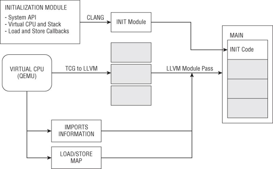
This initialization module implements load and store callbacks, declares system API prototypes, and sets a virtual processor unit and its stack.

The normalization module uses the information dynamically collected during target program execution to resolve imports, process relocations, and retrieve data sections. Import table information is used to build LLVM API call instructions. The load/store memory map is used to apply relocations and inject data from the target program into the LLVM module.

When the LLVM module is rebuilt, some additional optimization passes are applied to its representation. The LLVM can next be compiled to the chosen architecture, by using one of available LLVM back ends. It can also be translated to C or C++ code.

First results show that standard optimization used in conjunction with the partial evaluation induced by the dynamic translation of target code to its LLVM representation are sufficient to drastically reduce and simplify the code under analysis.

Final Thoughts

This section has discussed only four tools (and with a bias toward static analysis). Alongside the Metasm and Miasm frameworks, we could have cited the Radare framework (http://www.radare.org/y/), for example. Rolf Rolles's efforts to extend IDA with his idaocaml interpreter (https://code.google.com/p/idaocaml/) merit attention as well. There are plenty of others that we did not mention or only briefly mentioned here, and we encourage you to try them for yourself.

To put these tools into perspective, although IDA is a good disassembler, it cannot help much when it comes to dealing with obfuscated code. The Metasm and Miasm frameworks go a step further, offering more control, an IR to play with, and so on. Tools such as VxStripper go even further. You can probably feel it—there is an arms race going on. A huge amount of effort is put into the development of obfuscators, so our tools have to evolve as well.

As a reverse engineer, developing tools is an investment you make in order to fulfill your objectives; and you expect some sort of return on investment from it. Most advanced tools can take weeks if not months to build and require a lot of knowledge.

Practical Deobfuscation

Now you will see how some of the tools presented earlier can be used for practical deobfuscation. Again, there is no ambition of exhaustiveness in the following sections. Instead, the goal is to illustrate some common use cases of deobfuscation techniques.

Pattern-Based Deobfuscation

This may be the simplest and cheapest deobfuscation, operating at the syntactical level and matching known patterns. Don't forget that early obfuscation patterns were mainly manually crafted and protected code (like some packer code) and exhibited only a limited set of patterns; listing them all was thus “acceptable.”

This deobfuscation technique comes down to a search and replace algorithm at the binary (opcode) level (eventually using wildcard searching). The main drawback is that it leaves you with a binary plagued with NOP instructions.

To illustrate this, take a look at the following old OllyDbg script. Packers are a classic example of software using obfuscation techniques (in that case to protect their stubs). For years OllyDbg has been (and probably still is) the favorite tool for unpacking, and many scripts were released to assist in that task. This (random) old script (2004, by loveboom, http://tuts4you.com/download.php?view.601) targets ASProtect 2.0x versions (a commonly used packer at that time). It takes advantage of the OllyScript's REPL commands to search and replace a set of patterns. A REPL definition is as follows:

repl addr, find, repl, len

Replace find with repl starting att addr for len bytes.

All patterns are based on the same technique : an unconditional jump inside its successor instruction is used to confuse disassemblers. The diversity is slightly improved using instruction prefixes (like REP or REPNE). The repl instruction is used to replace these patterns with NOPs:

repl eip,#2EEB01??#,#90909090#,1000

repl eip,#65EB01??#,#90909090#,1000

repl eip,#F2EB01??#,#90909090#,1000

repl eip,#F3EB01??#,#90909090#,1000

repl eip,#EB01??#,#909090#,1000

repl eip,#26EB02????#,#9090909090#,1000

repl eip,#3EEB02????#,#9090909090#,1000

Here we only operate at the syntactic level. Considering a target with a limited set of patterns, this deobfuscation technique is trivial, however efficient:

· Application cost is limited if not negligible.

· Development cost is also almost null.

Of course, as with virus signatures and AV engines, polymorphism and diversity make it useless. An equivalent script could have been developed using IDA's scripting capabilities. That's typically the kind of script you can create when analyzing trivially obfuscated malware and/or packers, when speed of analysis has priority.

Program-Analysis-Based Deobfuscation

Now consider the following obfuscated code sample (this is only a very small extract; obfuscated code continues like this for thousands of instructions):

.text:00405900 loc_405900:

.text:00405900 add edx, 67E37DA7h

.text:00405906 push esi

.text:00405907 mov esi, 0D0B763Ah

.text:0040590C push eax

.text:0040590D mov eax, 15983FC8h

.text:00405912 neg eax

.text:00405914 inc eax

.text:00405915 inc eax

.text:00405916 jmp loc_4082AD

.text:004082AD loc_4082AD:

.text:004082AD not eax

.text:004082AF and eax, 1D48516Ch

.text:004082B4 sub eax, 0ACE1B37Ah

.text:004082B9 xor esi, eax

.text:004082BB pop eax

.text:004082BC xor edx, esi

.text:004082BE pop esi

.text:004082BF and ecx, edx

.text:004082C1 jmp loc_407C54

You likely recognize, from the first sections of this chapter, some of the obfuscation techniques used here, especially constant unfolding. Please also note that unconditional jumps are inserted to split code into basic blocks that are then distributed (randomly reordered) across the binary. There is no obvious pattern, at least none you could possibly and effectively match at the syntactical level using signatures.

You need to step up to the semantical level. Based on the output of a disassember, you could start working on the control flow, merging the basic blocks 405900h and 4082ADh. Then, you could work on the data flow, considering the two instructions:

.text:0040590D mov eax, 15983FC8h

.text:00405912 neg eax

Based on the semantics of these instructions, you know that the EAX register is first assigned with a constant value and then negged. You could precompute the NEG instruction and rewrite this in a simpler form, by assigning EAX with the negged value:

.text:0040590D mov eax, EA67C038h

Rewriting programs in a simpler form, precomputing values that do not depend on the program's input, removing useless code—that is program optimization, and compilers have done that almost since their creation. You can adapt and reuse these techniques for your own purposes, and an abundant body of literature is available on this topic. Some classical compiler optimization techniques include the following:

· Peephole optimization

· Constant folding/propagation

· Dead store elimination

· Operation folding

· Dead code elimination

· Etc.

This approach is exactly what is proposed by the Optimice deobfuscation plugin for IDA. Some previous works, by Gazet and Guillot²² and by Josse,²⁹ have also been presented, respectively as a Metasm plugin and a VxStripper plugin. The idea is to normalize the code in order to get a reduced/optimized/canonical form, which is simpler to analyze and closer to the original, unprotected, code.

These attempts to provide deobfuscation frameworks/utilities are still far from perfect. In addition, not many tools are available to the average reverser to attack obfuscated programs (of course, some private advanced tools exist here and there). The future of deobfuscation will probably take the form of elaborated tools and analysis platforms based on formal IR. Rolf Rolles presented some of his results with his own framework written in OCaml³⁴. Other popular frameworks that could be used include LLVM-based SecondWrite (Smithson et al., 2007³⁹), S2e/revgen (Chipounov, 2001⁷), or BitBlaze (Song et al., 2008⁴⁰ and their works since). Efforts in deobfuscation will have to match those put into obfuscation.

Complex Analysis

This section discusses two of the most impactful obfuscation techniques: code virtualization and code flattening. For these techniques, you clearly need to work at a semantic level.

Simple VM Implementations

There are mainly two forms of VM implementations. The most straightforward form is to develop a simple processor emulator. Algorithmically speaking, it would include the following steps:

1. Loop:

a. Fetch —Read the bytecode stream at the instruction pointer.

b. Decode—Decode the instruction's opcode and its operands.

c. Execute—Call the appropriate opcode handler.

2. Update the instruction pointer or exit the loop.

In this configuration, each instruction handler is responsible for updating the context of the VM. The context represents the underlying emulated architecture. It probably consists of a set registers, and eventually a memory area. Each handler implements a distinctive instruction of the emulated processor (one handler for the ADD, one for the SUB, etc.).

This form is often used by the simpler implementations. Handlers are totally independent of one another, and the instruction pointer is increased by the size of the instruction (except for instructions that directly modify it).

From an attacker's point of view, this type of implementation is easily recognizable. Following is a detailed look at the steps generally required to analyze a VM:

1. Understand how an instruction is decoded from raw bytecode: which part encodes for the operation (handler number), which part encodes the operand(s), and so on.

2. Deduct VM's architecture from instructions' operands: number of registers, memory layout, I/O interfaces, etc.

3. Undertake handler analysis. Once operand decoding is known, you can look at the way each handler manipulates the various operand(s) it possibly takes as argument(s). This step is the essence of VM analysis: Each handler is associated with its own semantics.

With all these pieces of knowledge, you can finally build a disassembler-like tool that enables you to disassemble the bytecode of the VM.

In 2006, Maximus published two great papers about VM reversing: “Reversing a simple virtual machine”³² and “Virtual machines re-building”³³. One of the targets he used (HyperUnpackme2) was also covered in depth by Rolf Rolles the same year³⁵.

Although these are useful contributions from talented reversers, VM analysis remains a somewhat manual and repetitive job: One has to develop a new disassembler for each new instance of VM. Moreover, protections authors have also reacted, hardening their implementations of VMs.

Advanced VM Implementations

More advanced VM implementations derive from the simple type but add important features to harden the implementations and make them more resilient to analysis:

· Loop unrolling—This classical compiler optimization technique favors the time (speed) aspect of a program's space vs. time trade-off. It replaces the loop structure by the sequential invocations of the loop body (thus unrolled). Applied to a VM, each handler is made responsible for fetching and decoding its own operand(s), and then updates the context accordingly.

· Code-flattening—The VM's main execution loop is flattened. That means each handler is responsible for updating the instruction pointer (pointer on the bytecode). Actually, code-flattening and VM-based obfuscation are basically the same thing. Code-flattening only virtualizes/retargets the control flow of the protected code, whereas virtual-machine obfuscation virtualizes/retargets both the control flow and the data flow. You can use almost the same algorithms to follow a code-flatten dispatcher's context and a VM context.

· Bytecode encoding/encryption—Each invocation of the VM depends on an encryption key that is passed to the VM as part of its context initialization. Each handler updates that key, resulting in a turning key. The handlers depend on the turning key to decode their operands from encoded bytecode. An attacker cannot start analyzing the VM at a chosen point, as the value of the key at this point would be unknown.

· Code obfuscation—The native code of the VM is obfuscated using techniques like the one described at the beginning of this chapter. Simply looking at a handler's code provides no clue about its semantics.

In summary, hardened implementations of VMs are more difficult to analyze statically by an order of magnitude. For each state of the VM, an attacker has to know at least the following mandatory values:

· Bytecode pointer

· Instruction pointer, the value of the next handler to be executed

· Turning encryption key

VMs have reached a new level of complexity, thus necessitating a new level of attack. Handlers are more complex to analyze; moreover, they cannot be analyzed in isolation (one would not know the value of the encryption key, for example). An attacker wants to limit the manual analysis to a minimum. Nevertheless, a manual review is most often required to “capture” the general behavior of a VM and thus infer possible attacks on it.

One of the first places of interest is the VM invocation stub—i.e., the transition between native (nonvirtualized) code and the VM/interpreter. The context initialization indicates the nature of the mapping between the native architecture and the VM's architecture. It may be a carbon copy of native registers to the VM's registers or something more complicated. Also, at this point, it is helpful to distinguish (as much as possible) between mandatory initialization variables (such as a VM's key, handler number, or entry point) for which a numerical value is required, and extra variables that can be kept symbolic.

The second place of major interest is the VM's dispatcher (if it exists). Most often there is a single point of dispatch that basically retrieves the next handler from a handlers table based on an index stored somewhere within the VM's context. A question to answer is, what is the break condition of this execution loop? In this configuration it is possible to consider the VM as a generalization of code-flattening. Code-flattening virtualizes only the control flow, whereas the VM virtualizes both the control and data flows. Moreover, code-flattening most often only operates at single function level, whereas the VM operates at the program level. The other possibility is a distributed dispatch, whereby each handler is responsible for updating the VM's instruction pointer and linking to the next handler.

These are general ideas; each reverser has his or her own tricks and abstractions of the problem.

Using Metasm

The approach we are going to explore is based on the Metasm framework. It relies on symbolic execution to make the VM (i.e., interpreter) process the bytecode (with respect to static data) and compute the residual program. On the one hand, there is a program (the interpreter); on the other hand, there is its static data (the bytecode); we will specialize the program with respect to its static data.

Considering an obfuscated program and its data as a whole would be too complex, the solution is to break this complex problem into multiple, simpler sub-problems. Considering virtual machine's instruction handlers level provides a far more appropriate granularity. From now on, we will consider instruction handlers as the interpreter's smallest unit of semantics.

Based on that basic premise, you can apply the following pseudo algorithm:

1. Capture the current context (VM's bytecode, static parameters, known environment, etc.).

2. Disassemble the current handler.

3. Deobfuscate code, if necessary.

4. Compute its semantics (i.e., transfer function).

5. Generate output from solved semantics.

6. Compute next state (i.e., apply the transfer function to the current context).

7. If the handler's dispatcher doesn't reach a break/exit condition, repeat from step 1.

Optionally, you may be able to regenerate native code from the transfer function computed at step 4. As expressed by Futamura²¹, given an interpreter of L_interpreted written in a given native language L_native , it is possible to automatically compute a compiler from L_interpreted to L_native.

This is suitable for the theoretical concepts. Now suppose that you face an instance of a VM. Where do you start? Let's take a practical example.

The following script makes use of Metasm to compile and then disassemble what could be a handler from a VM. For the sake of simplicity, this example deals only with the VM's part (thus, code is not obfuscated). The handler's code is located in 10000000h, while a data section containing the handler's bytecode is located in 1a000000h:

# encoding: ASCII-8BIT

#!/usr/bin/env ruby

require "metasm"

include Metasm

$SPAWN_GUI = false

CODE_BASE_ADDR = 0x10000000

HTABLE_BASE_ADDR = 0x18000000

DATA_BASE_ADDR = 0x1A000000

INJECT_MAX_ITER = 0x20

NATIVE_REGS = [:eax, :edx, :ecx, :ebx, :esp, :ebp, :esi, :edi]

def display(bd)

bd.each{|key,value| puts " #{Expression[key]} => #{Expression[value]}"}

end

# produce handler's x86 code

sc = Metasm::Shellcode.assemble(Metasm::Ia32.new, EOS)

lodsd

mov ecx, eax

xor ecx, ebp

movzx eax, cl

push eax

mov eax, [edi+eax]

movzx edx, ch

mov edx, [edi+edx]

xor eax, edx

pop edx

mov [edi+edx], eax

lodsd xor ebp, 0x35ef6a14

xor eax, ebp

jmp [#{HTABLE_BASE_ADDR}+eax*4]

EOS

handler = sc.encode_string

# data section hex

data_section_hex = "\xA3\xCB\xDB\x5F\x60\xBD\x34\x6A"

# add a code section

dasm = sc.init_disassembler

dasm.add_section(EncodedData.new(handler), CODE_BASE_ADDR)

# add a data section

dasm.add_section(EncodedData.new(data_section_hex), DATA_BASE_ADDR)

# disassemble handler code

dasm.disassemble_fast_deep(CODE_BASE_ADDR)

The first thing to do is automatically get the semantics of that handler. As mentioned previously, Metasm offers a method called code_binding that computes the function transfer (Metasm's terminology is binding) of a set of instructions. Thus, you can write the following:

# compute handler's semantics

bb = dasm.di_at(CODE_BASE_ADDR).block

start_addr = bb.list.first.address

end_addr = bb.list.last.address

puts "[+] from 0x#{start_addr.to_s(16)}, to 0x#{end_addr.to_s(16)}"

binding = dasm.code_binding(start_addr, end_addr)

display(binding)

The preceding produces the following output:

[+] from 0x10000000, to address 10000021

dword ptr [esp] => (dword ptr [esi]^ebp)&0ffh

dword ptr [edi+((dword ptr [esi]^ebp)&0ffh)] =>

dword ptr [edi+((dword ptr[esi]^ebp)&0ffh)] ^

dword ptr [edi+(((dword ptr[esi]8)^(ebp8))&0ffh)]

eax => (dword ptr [esi+4]^(ebp^35ef6a14h))&0ffffffffh

ecx => (dword ptr [esi]^ebp)&0ffffffffh

edx => (dword ptr [esi]^ebp)&0ffh

ebp => (ebp^35ef6a14h)&0ffffffffh

esi => (esi+8)&0ffffffffh

From both the assembly and the binding, you can say the following about the VM:

· It seems to use a turning key store in EBP. (Note how it is used to decrypt the instruction's operands from bytecode.)

· Its context seems to be pointed to by EDI.

That's a good start, but you are still far from the objective. You are still stuck at the assembly level, so let's step back and consider the VM initialization, which we have identified as follows:

pushad

pop [edi]

pop [edi+0x4]

pop [edi+0x8]

pop [edi+0xC]

pop [edi+0x10]

pop [edi+0x14]

pop [edi+0x18]

pop [edi+0x1C]

First, native registers are pushed onto the stack, and then they are read from the stack into a memory area pointed to by EDI, which in turn is responsible for pointing at the VM's context. This information enables you to create a mapping between the VM's symbolic internals and assembly expression:

vm_symbolism = {

:eax => :nhandler,

:ebp => :vmkey,

:esi => :bytecode_ptr,

Indirection[[:edi], 4, nil] => :vm_edi,

Indirection[[:edi, :+, 4], 4, nil] => :vm_esi,

Indirection[[:edi, :+, 8], 4, nil] => :vm_ebp,

Indirection[[:edi, :+, 0xC], 4, nil] => :vm_esp,

Indirection[[:edi, :+, 0x10], 4, nil] => :vm_ebx,

Indirection[[:edi, :+, 0x14], 4, nil] => :vm_edx,

Indirection[[:edi, :+, 0x18], 4, nil] => :vm_ecx,

Indirection[[:edi, :+, 0x1c], 4, nil] => :vm_eax,

}

This symbolism is injected into the binding (each occurrence of a left value is replaced by its associated right value). Expressions have a special method named bind that does exactly that. The following example first defines a symbolic expression: the addition of two terms, one of them being an indirection; and two symbols are involved, :a and :b. Next, symbol :a is associated (bound) with the value 1000h:

expr = Expression[[:a, 4], :+, :b]

sym = {:a => 0x1000}

puts expr

dword ptr [a]+b

puts expr.bind(sym)

dword ptr [1000h]+b

You can generalize this for each expression of the binding. This mapping is the key that enables abstracting VM's code from its implementation level up to the VM semantics level. Moreover, a positive side effect of this step is often a significant reduction of the binding's complexity. The new binding is as follows:

[+] symbolic binding

dword ptr [esp] => (dword ptr [bytecode_ptr]^vmkey)&0ffh

dword ptr [edi+((dword ptr [bytecode_ptr]^vmkey)&0ffh)] =>

dword ptr [edi+dword ptr [bytecode_ptr]^vmkey)&0ffh)]^

dword ptr[edi+(((dword ptr [bytecode_ptr]8)^(vmkey8))&0ffh)]

nhandler => (dword ptr [bytecode_ptr+4]^(vmkey^35ef6a14h))&0ffffffffh

vmkey => (vmkey^35ef6a14h)&0ffffffffh

bytecode_ptr => (bytecode_ptr+8)&0ffffffffh

We have made progress, but the encryption is still problematic and we cannot go further if the VM's context at the execution time of this handler is unknown: bytecode pointer, turning key, and optionally the handler number are all required values. Assuming you know these values (you are at the VM's entry point or you have dynamically traced the VM up to that point), you can define a pseudo-context:

context = {

:nhandler => 0x84,

:vmkey => 0x5fdbd7b7,

:bytecode_ptr => DATA_BASE_ADDR,

:virt_eax => 0xffeeffee,

:virt_ecx => 0,

:virt_edx => 0x41414141,

:virt_ebx => 1,

:virt_edi => :virt_edi,

}

Note that the context contains both symbolic and numerical values. For example, nhandler is defined as equal to 84h, while the VM's register virt_edi is symbolic.

The context is then injected within the binding, as well as the symbolism defined previously. In practice that's an iterative process, but let's not get overloaded with implementation details. Expressions are progressively solved and reduced with respect to all known values, which include the current context and the program's data (i.e., the bytecode). At the end you have a solved binding, which actually represents the context of the VM after the execution of the handler. We call that step symbolic execution:

[+] binding solver

[+] key: dword ptr [esp]

=> solved key: dword ptr [esp]

[+] value: (dword ptr [bytecode_ptr]^vmkey)&0ffh

[+] solved memory read at 0x1a000000, size 4

[+] value 5fdbcba3h

=> solved value: 14h

[+] key: dword ptr [edi+((dword ptr [bytecode_ptr]^vmkey)&0ffh)]

[+] solved memory read at 0x1a000000, size 4

[+] value 5fdbcba3h

=> solved key: virt_edx

[+] value: dword ptr [edi+((dword ptr [bytecode_ptr]^vmkey)&0ffh)]^

dword ptr [edi+(((dword ptr [bytecode_ptr]8)^(vmkey8))&0ffh)]

[+] solved memory read at 0x1a000000, size 4

[+] value 5fdbcba3h

[+] solved memory read at 0x1a000000, size 4

[+] value 5fdbcba3h

=> solved value: 0beafbeafh

[+] key: nhandler

=> solved key: nhandler

[+] value: (dword ptr [bytecode_ptr+4]^(vmkey^35ef6a14h))&0ffffffffh

[+] solved memory read at 0x1a000004, size 4

[+] value 6a34bd60h

=> solved value: 0c3h

[+] key: vmkey

=> solved key: vmkey

[+] value: (vmkey^35ef6a14h)&0ffffffffh

=> solved value: 6a34bda3h

[+] key: bytecode_ptr

=> solved key: bytecode_ptr

[+] value: (bytecode_ptr+8)&0ffffffffh

=> solved value: 1a000008h

[+] solved binding

virt_edx => 0beafbeafh

nhandler => 0c3h

vmkey => 6a34bda3h

bytecode_ptr => 1a000008h

The expression solver helps to compute the final values of the first handler's binding: the next handler to be executed as well as the updated value of the turning key. Updating the context is a trivial operation:

updated_context = context.update(solved_binding)

puts "\n[+] updated context"

display(updated_context)

[+] updated context

nhandler => 0c3h

vmkey => 6a34bda3h

bytecode_ptr => 1a000008h

virt_eax => 0ffeeffeeh

virt_ecx => 0

virt_edx => 0beafbeafh

virt_ebx => 1

virt_edi => virt_edi

You can repeat this process and walk through the whole control-flow graph of the VM. This is a quite appreciable result; nevertheless, pure numerical values somewhat hide the semantics of the handler. Moreover, one of the objectives is to regenerate native assembly code equivalent to the contextualized execution of the handler.

A trick we often use when analyzing a VM with Metasm is to proceed to a double symbolic execution for each handler: one with the full context (mainly numerical values, used to update the context) and another one with an almost purely symbolic context (used to extract the high-level semantics). The next code sample demonstrates the use of a symbolic context:

symbolic_context = {

:nhandler => 0x84,

:vmkey => 0x5fdbd7b7,

:bytecode_ptr => DATA_BASE_ADDR,

:virt_eax => :virt_eax,

:virt_ecx => :virt_ecx,

:virt_edx => :virt_edx,

:virt_ebx => :virt_ebx,

:virt_edi => :virt_edi,

}

solved_symolic_binding = sym_exec(symbolic_context,

symbolic_binding,

vm_symbolism)

puts "\n[+] solved binding" display(solved_symbolic_binding)

This time the output is as follows:

[+] binding solver

[+] key: dword ptr [esp]

=> solved key: dword ptr [esp]

[+] value: (dword ptr [bytecode_ptr]^vmkey)&0ffh

[+] solved memory read at 0x1a000000, size 4

[+] value 5fdbcba3h

=> solved value: 14h

[+] key: dword ptr [edi+((dword ptr [bytecode_ptr]^vmkey)&0ffh)]

[+] solved memory read at 0x1a000000, size 4

[+] value 5fdbcba3h

=> solved key: virt_edx

[+] value: dword ptr [edi+((dword ptr [bytecode_ptr]^vmkey)&0ffh)]^

dword ptr edi+(((dword ptr [bytecode_ptr]8)^(vmkey8))&0ffh)]

[+] solved memory read at 0x1a000000, size 4

[+] value 5fdbcba3h

[+] solved memory read at 0x1a000000, size 4

[+] value 5fdbcba3h

=> solved value: virt_edx^virt_eax

[+] key: nhandler

=> solved key: nhandler

[+] value: (dword ptr [bytecode_ptr+4]^(vmkey^35ef6a14h))&0ffffffffh

[+] solved memory read at 0x1a000004, size 4

[+] value 6a34bd60h

=> solved value: 0c3h

[+] key: vmkey

=> solved key: vmkey

[+] value: (vmkey^35ef6a14h)&0ffffffffh

=> solved value: 6a34bda3h

[+] key: bytecode_ptr

=> solved key: bytecode_ptr

[+] value: (bytecode_ptr+8)&0ffffffffh

=> solved value: 1a000008h

[+] solved binding

virt_edx => virt_edx^virt_eax

nhandler => 0c3h

vmkey => 6a34bda3h

bytecode_ptr => 1a000008h

Finally, you can simply reject VM control stuff from the solved binding, leaving you with the following:

vm_edx => vm_edx^vm_eax

From that final result, native code regeneration is pretty straightforward. You iterate this process over the VM's control-flow graph for each handler. As a general observation, when using this technique, a sensitive choice is when to keep symbolic values and when to reduce to numerical values. The first option favors the recovery of high-level semantics, while the second enables an easier VM's control-flow recovery. At the end, it is also possible to further proceed the output. Imagine a VM that looks like a stack-based interpreter:

01: push vm_edx

02: add [esp], vm_eax

03: pop vm_edx

Using classic deobfuscation methods such as compiler optimizations would rewrite the preceding three lines as follows:

01: add vm_eax, vm_eax

Please note that the bytecode itself could have been obfuscated.

Code-Flattening Deobfuscation

As previously stated, code-flattening can be viewed as partial virtualization (only the control flow is virtualized). Thus, techniques described for VM analysis, and especially symbolic execution, can also be applied for flattened code analysis.

There are still some difficulties that are specific to this technique:

· Code-flattening transformation is most often applied at the function level and sometimes there may be more than one flattened “node” in the same function. Overall that means there are multiple instances of the techniques; thus a tool has to be bulletproof and fully automatic.

· Discerning between a function's original code and added dispatcher's code is difficult when code-flattening implementation is robust (program and dispatcher data flows are firmly interleaved /interdependent).

· Inverse transformation is not trivial to implement.

Using VxStripper

To illustrate the use of VxStripper on a simple “toy” example, consider the following program (which displays y = 22) after unpacking and reconstruction:

...... ! entrypoint:

...... ! push ebp

401001 ! mov ebp, esp

401003 ! sub esp, 10h

401006 ! mov dword ptr [ebp-4], 0

40100d ! mov dword ptr [ebp-0ch], 2

401014 ! mov dword ptr [ebp-8], 0ah

40101b !

...... ! loc_40101b:

...... ! cmp dword ptr [ebp-0ch], 6

40101f ! jnl loc_40108c

401021 ! mov eax, [ebp-0ch]

401024 ! mov [ebp-10h], eax

401027 ! mov ecx, [ebp-10h]

40102a ! sub ecx, 2

40102d ! mov [ebp-10h], ecx

401030 ! cmp dword ptr [ebp-10h], 3

401034 ! ja loc_40108a

401036 ! mov edx, [ebp-10h]

401039 ! jmp dword ptr [edx*4+data_4010a4]

401040 mov dword ptr [ebp-4], 2

401047 mov dword ptr [ebp-0ch], 3

40104e jmp loc_40108a

401050 cmp dword ptr [ebp-8], 0

401054 jng 40105fh

401056 mov dword ptr [ebp-0ch], 4

40105d jmp 401066h

40105f mov dword ptr [ebp-0ch], 6

401066 jmp loc_40108a

401068 mov eax, [ebp-4]

40106b add eax, 2

40106e mov [ebp-4], eax

401071 mov dword ptr [ebp-0ch], 5

401078 jmp loc_40108a

40107a mov ecx, [ebp-8]

40107d sub ecx, 1

401080 mov [ebp-8], ecx

401083 mov dword ptr [ebp-0ch], 3

40108a !

...... ! loc_40108a:

...... ! jmp loc_40101b

40108c !

...... ! loc_40108c:

...... ! mov edx, [ebp-4]

40108f ! push edx

401090 ! push strz_yd_402008

401095 ! call dword ptr [msvcrt.dll:printf]

40109b ! add esp, 8

40109e ! xor eax, eax

4010a0 ! mov esp, ebp

4010a2 ! pop ebp

4010a3 ! ret return 0;

The control-flow graph (CFG) of such a program is flattened.

The normalization module's execution produces (when you do not apply all optimizations) the following code:

...... ! push eax

4011f1 ! mov dword ptr [esp-0ch], 0ah

4011f9 ! mov dword ptr [esp-8], 4

401201 ! dec dword ptr [esp-0ch]

401205 ! add dword ptr [esp-8], 2

40120a ! dec dword ptr [esp-0ch]

40120e ! add dword ptr [esp-8], 2

401213 ! dec dword ptr [esp-0ch]

401217 ! add dword ptr [esp-8], 2

40121c ! dec dword ptr [esp-0ch]

401220 ! add dword ptr [esp-8], 2

401225 ! dec dword ptr [esp-0ch]

401229 ! add dword ptr [esp-8], 2

40122e ! dec dword ptr [esp-0ch]

401232 ! add dword ptr [esp-8], 2

401237 ! dec dword ptr [esp-0ch]

40123b ! add dword ptr [esp-8], 2

401240 ! dec dword ptr [esp-0ch]

401244 ! add dword ptr [esp-8], 2

401249 ! dec dword ptr [esp-0ch]

40124d ! add dword ptr [esp-8], 2

401252 ! dec dword ptr [esp-0ch]

401256 ! mov eax, [esp-8]

40125a ! mov [esp-18h], eax

40125e ! mov dword ptr [esp-1ch], strz_yd_402010

401266 ! mov ebp, esp

401268 ! lea eax, [esp-1ch]

40126c ! mov esp, eax

40126e ! call crtdll.dll:printf_4012d8

401273 ! mov esp, ebp

401275 ! mov ebp, esp

401277 ! lea eax, [esp+8]

40127b ! mov esp, eax

40127d ! mov esp, ebp

40127f ! xor eax, eax

401281 ! pop edx

401282 ! ret

Note that the dynamic generation of code performed by VxStripper naturally unflattens the flattened code. Applying standard optimization transformations results in a program stripped of this obfuscation:

...... ! push eax

4011f1 ! mov dword ptr [esp-18h], 16h

4011f9 ! mov dword ptr [esp-1ch], strz_yd_402010

401201 ! mov ebp, esp

401203 ! lea eax, [esp-1ch]

401207 ! mov esp, eax

401209 ! call crtdll.dll:printf_401268

40120e ! mov esp, ebp

401210 ! mov ebp, esp

401212 ! lea eax, [esp+8]

401216 ! mov esp, eax

401218 ! mov esp, ebp

40121a ! xor eax, eax

40121c ! pop edx

40121d ! ret

Even if work remains before obtaining software that supports the set of software protection tools usable by malware authors, these first results encourage us to pursue the study of generic methods of unpacking and normalization, with the goal of automating as much as possible the tasks conducted by an analyst.

This tool provides a self-sufficient piece of software for malware analysis. However, one of the future goals of this project is to enable the tool to interact with other analysis tools. By design, this tool may be able to collaborate with any software analysis tool based on the LLVM compilation chain.

The LLVM compilation chain and the many LLVM-based tools already provide a great library of program analyses that can be used together to defeat malware protection mechanisms.

In addition, Vellvm (Verified LLVM) may be used to formally extract verified implementations of deobfuscation passes implemented by VxStripper. In addition to malware threat analysis, other uses of this tool can also be imagined, such as detection scheme extraction, software protections, and antivirus software robustness analysis.

Case Study

The sample we'll use for this case study is actually a crackme originally posted on Crackmes.de by quetz in 2007. Even though it is a “only” a crackme, it features most of the concepts that one would find in a professional-grade protection. Among other rejoicings it contains the following:

· Code-flattening

· Variable encoding

· Code virtualization

Here is how the author introduces its challenge:

Lately, protection from static analysis becomes more and more popular. Almost every protector employs some kind of obfuscation, virtual machine, etc… This keygenme is an attempt to show what happens if you abuse idea of obfuscation. Can human effectively analyze such code? Maybe with an assistance of a tool?

—http://crackmes.de/users/quetz/q_keygenme_1.0/

Fortunately, we have tools and in this section we will use them. Before starting, we recommend that you not look at the symbols section contained within the binary. As an aside, previous versions of IDA Pro (maybe inferior to 6.2) didn't load these symbols and the author of these lines cheerfully failed to look for them.

First Impressions

Launching the executable offers you the opportunity to input a username and a password. After clicking the Check button, a message box appears and displays the validity of your credentials.

If you've carefully read the previous chapters of this book, you have probably already fired up your favorite disassembler and targeted the GUI's DialogProc callback function.

Let's first look at the general architecture of the protected code. The control-flow graph is way too messy to be natural compiler-generated code: We have an obfuscated DialogProc calling two code-flattened functions (func1@0x430DB0, func2@0x431E00). These two functions themselves call what seems to be a VM (vm@0x401360).

We have already discussed the VM's single dispatch point; this one is pretty straightforward to spot (look for an important jump table in the absence of any other clues):

01: .text:00401F20

02: mov ebp, [esp+13Ch]

03: cmp ebp, 3E2Dh; switch 15918 cases

04: ja short loc_401F36

05: jmp ds:off_43D000[ebp*4]; switch jump

These are our two first and almost free pieces of knowledge about the VM: It stores its current handler number in [ESP+13Ch] and there are 15,918 entries in the dispatcher (for now, we cannot conclude whether they are all different handlers).

Before getting our hands dirty, we can try to do some black-box analysis of the func1 and func2 functions. We know func1 and func2 call the VM; we simply log every call to the VM and especially the number of the first handler that is called (a sort of entry point in the VM code). That seems quite trivial but one should never disregard low-hanging fruit.

Results are immediately revealing: func2 is called before func1, so we will start with func2. As soon as you look at the logs of the VM's entry point, these patterns stand out:

· 546h-0BFFh-7B2h-9A2h-405h-919h-3B9h—624 times

· 0CF5h-15Eh-184h-39Ch-5B0h-3C0h-0F75h—624 times

· 0A06h-0xA29h-0x268h-0xCB3h—227 times

· 736h-13Ah-1EBh-897h—396 times

· 150h-8ABh-843h-697h-474h—200 times

That's actually already a lot of information. If you look at the .data section, an extra hint is waiting:

01: .data:0043CA44 dword_43CA4402: .data:0043CA48 dd 9908B0DFh

Where does 9908B0DFh come from? And 624? And 227? Well, either you are really familiar with random number generators or you look for these values; they identify a Mersenne twister pseudo-random generator algorithm. 624 and 397 are the period parameters, while 9908B0DFh is a constant used during number generation.

We have identified a critical weakness of the protection: Virtualized code leaks some information about the structure of the protected algorithm, making it trivial to recover loop iterations. Nevertheless, do we have nicely crafted virtualized code nullified with one breakpoint? Not yet. We have an algorithm candidate but it needs to be confirmed.

Again, one should never reverse engineer some code when it is possible to guess (and validate) information! In this case, a black-box analysis reveals a lot simply by looking at the inputs/outputs of functions func1 and func2. A basic strategy like this or differential analysis of VM execution can sometimes be of great help. Let's refine our analysis of these two functions:

· func2

· Input—Two arguments: an address on the stack that seems to be an array of integers, and a 32-bit value that seems to depend on the length of the name.

· Output—Nothing remarkable except that the integers array has been updated.

· Occurrence—Called a single time, at the beginning and before func1.

· Guess—Mersenne twister initialization, the array is actually the state of the PNRG. The 32-bit value is the initialization seed. This can be further validated by matching loop parameters (learned from the logs) with a standard initialization function.

· func1

· Input—Two arguments: the address of the (supposed) PRNG state and a 32-bit value that seems to be a letter from the username.

· Output—Returns a 32-bit random value.

· Occurrence—Called 100 times.

· Guess—Mersenne twister rand32-like function.

Analyzing Handlers Semantics

It is now time to analyze the VM. The main dispatcher has already been found at [ESP+13ch]. It is often a good idea to manually check a few handlers to see how they access the VM's context, how they update the program counter and/or bytecode pointer, and so on.

This process can be applied on a random handler—for example, the one starting at 0x41836c:

01: .text:0041836C loc_41836C:

02: ; DATA XREF: .rdata:off_43D000

03: ; jumptable 00401F2F cases 2815,4091

04: .text:0041836C movzx ecx, [esp+3D8h+var_2A2]

05: .text:00418374 mov esi, 97Fh

06: .text:00418379 mov ebx, [esp+3D8h+var_3C8]

07: .text:0041837D movzx edi, [esp+3D8h+var_29E]

08: .text:00418385 add [esp+3D8h+var_3C0], 94Eh

09: .text:0041838D imul eax, ecx, 1Ch

10: .text:00418390 sub [esp+3D8h+var_3C4], 0FF0h

11: .text:00418398 imul ecx, edi, 5DDh

12: .text:0041839E mov [esp+3D8h+var_37C], esi

13: .text:004183A2 lea edx, [eax+ebx+5C8h]

14: .text:004183A9 mov ebx, 97Fh

15: .text:004183AE mov [esp+3D8h+var_3C8], edx

16: .text:004183B2 sub ebx, ecx

17: .text:004183B4 lea edx, [ebp+ebx+29Dh+var_8BC]

18: .text:004183BB mov [esp+3D8h+var_378], ebx

19: .text:004183BF mov [esp+3D8h+var_380], ebx

20: .text:004183C3 mov [esp+3D8h+var_29D+1], edx

21: .text:004183CA jmp loc_401F20

Let's get some help from Metasm. As shown previously, we can use the code-binding method to compute the semantics of a chunk of code:

dword ptr [esp+10h] => 1ch*byte ptr [esp+136h]+dword ptr [esp+10h]+5c8h

dword ptr [esp+14h] => dword ptr [esp+14h]-0ff0h

dword ptr [esp+18h] => dword ptr [esp+18h]+94eh

dword ptr [esp+58h] => -5ddh*byte ptr [esp+13ah]+97fh

dword ptr [esp+5ch] => 97fh

dword ptr [esp+60h] => -5ddh*byte ptr [esp+13ah]+97fh

dword ptr [esp+13ch] => ebp-5ddh*byte ptr [esp+13ah]+360h

eax => (1ch*byte ptr [esp+136h])&0ffffffffh

ecx => (5ddh*byte ptr [esp+13ah])&0ffffffffh

edx => (ebp-5ddh*byte ptr [esp+13ah]+360h)&0ffffffffh

ebx => (-5ddh*byte ptr [esp+13ah]+97fh)&0ffffffffh

esi => 97fh

edi => byte ptr [esp+13ah]&0ffffffffh

The VM's context is stored on the stack and no values are passed by registers between handlers; that means all register modification can be dropped to get a clearer view:

dword ptr [esp+10h] => 1ch*byte ptr [esp+136h]+dword ptr [esp+10h]+5c8h

dword ptr [esp+14h] => dword ptr [esp+14h]-0ff0h

dword ptr [esp+18h] => dword ptr [esp+18h]+94eh

dword ptr [esp+58h] => -5ddh*byte ptr [esp+13ah]+97fh

dword ptr [esp+5ch] => 97fh

dword ptr [esp+60h] => -5ddh*byte ptr [esp+13ah]+97fh

dword ptr [esp+13ch] => ebp-5ddh*byte ptr [esp+13ah]+360h

We already know that the handler number is stored at [ESP+13Ch]. It is updated by the handler. Its final value depends on the value of byte ptr [ESP+13ah]. By analyzing a few other handlers, we can guess it is a Boolean value, and a few other Booleans are stored in the context. This one is stored in second position, and it will be named flag2.

[ESP+58h], [ESP +5Ch], and [ESP +60h] are firmly tied with the handler number computation. They respectively contain the delta between the old and new handler number in case the condition (here flag2) is true or false.

[ESP +10h], [ESP +14h], and [ESP +18h] are also of high interest. They are updated by almost every handler and are supposed to decrypt the bytecode: They access the large undefined constants table stored in the .data section). They are actually like a running key; they'll be named respectivelykey_a, key_b, and key_c.

The following is an example of key usage taken from handler 0xa0a at address 0x427b17:

nHandler => dword ptr [4*key_c+436010h]^

dword ptr [4*key_b+436010h]^

dword ptr [4*key_a+436010h]

The names can be injected within the handler's binding, making it more understandable (even if that's not our main objective here) and easy to manipulate:

key_a => 1ch*flag6+key_a+5c8h

key_b => key_b-0ff0h

key_c => key_c+94eh

delta_true => -5ddh*flag2+97fh

delta_false => 97fh

delta => -5ddh*flag2+97fh

nHandler => ebp-5ddh*flag2+360h

This handler has almost the semantics of a conditional jump. By analyzing a few other handlers, it is possible to recover and validate a mapping of the VM's symbolic variables, which will be represented by a hash object:

SYMBOLIC_VM = {

Indirection[Expression[ :esp, :+, 0x10], 4, nil] => :key_a,

Indirection[Expression[ :esp, :+, 0x14], 4, nil] => :key_b,

Indirection[Expression[ :esp, :+, 0x18], 4, nil] => :key_c,

Indirection[Expression[ :esp, :+, 0x58], 4, nil] => :delta,

Indirection[Expression[ :esp, :+, 0x5c], 4, nil] => :delta_false,

Indirection[Expression[ :esp, :+, 0x60], 4, nil] => :delta_true,

Indirection[Expression[ :esp, :+, 0x134], 1, nil] => :flag8,

Indirection[Expression[ :esp, :+, 0x135], 1, nil] => :flag7,

Indirection[Expression[ :esp, :+, 0x136], 1, nil] => :flag6,

Indirection[Expression[ :esp, :+, 0x137], 1, nil] => :flag5,

Indirection[Expression[ :esp, :+, 0x138], 1, nil] => :flag4,

Indirection[Expression[ :esp, :+, 0x139], 1, nil] => :flag3,

Indirection[Expression[ :esp, :+, 0x13a], 1, nil] => :flag2,

Indirection[Expression[ :esp, :+, 0x13b], 1, nil] => :flag1,

Indirection[Expression[ :esp, :+, 0x13c], 4, nil] => :nHandler

}

Other memory locations do not seem to have a dedicated purpose; they can be considered/mapped as general-purpose registers. With this mapping, we have all we need to process a symbolic execution of the VM (i.e., step-by-step execution of handler's semantics).

Symbolic Execution

In order to process a symbolic execution, you must have some clues about the initialization context of the VM; recall the initial value of the turning key or the value of the program counter (handler number). In our case, calls to the VM are themselves obfuscated (remember the previously discussed graph-flattened functions), making the initialization context quite hard to recover statically. In that situation, one can simply take the best of the two worlds and use a compromise between static and dynamic analysis, sometimes referred to as concolic execution.

Basically that means you debug the target and catch (break at) every call to the VM; within the callback, you switch from dynamic to static analysis and proceed to the following actions:

1. Dump target's memory.

2. Initialize the symbolic analysis context with the memory dump. Actually, a kind of lazy loading can be used. All access to the uninitialized context will be solved and cached using the memory dump.

3. Compute the VM's symbolic execution.

Using concolic execution, it becomes quite easy to follow the execution flow of the VM (i.e., a succession of handlers). The process of handler analysis and tracing is fully automated.

Here is an example of output of the tool for one handler. The extensive use of the turning key (consisting of key_a, key_b, and key_c) clearly appears; in this situation, the key is used to obfuscate access to the VM's context:

[+] disasm handler 2be at 42c2cdh

[+] analyzing handler at 0x42c2cd

[+] considering code from 0x42c2cd to 0x42c3b3

[+] cached handler binding

dword ptr [dword ptr [esp+4*(dword ptr [4*key_b+436000h]^

(dword ptr [4*key_c+436000h]^dword ptr [4*key_a+436000h]))+140h]] =>

dword ptr [dword ptr [esp+4*(dword ptr [4*key_b+436004h]^

(dword ptr [4*key_c+436004h]^dword ptr [4*key_a+436004h]))+140h]]

key_c => key_c+5

key_b => key_b+5

key_a => key_a+5

nHandler => (dword ptr [4*key_b+43600ch]^

(dword ptr [4*key_c+43600ch]^dword ptr [4*key_a+43600ch]))+

(((dword ptr [4*key_c+436010h]^(dword ptr [4*key_b+436010h]^

dword ptr [4*key_a+436010h]))*(byte ptr [dword ptr [esp+4*

(dword ptr [4*key_b+436008h]^(dword ptr [4*key_c+436008h]^

dword ptr [4*key_a+436008h]))+140h]]&0ffh))&0ffffffffh)

[+] symbolic binding

dword ptr [esp+0a8h] => dword ptr [esp+0ach]

key_c => 0d6h

key_b => 1f6h

key_a => 126ah

nHandler => ((21eh*(flag4&0ffh))&0ffffffffh)+0ac6h

[+] solved binding

dword ptr [esp+0a8h] => 4f3de0b9h

key_c => 0d6h

key_b => 1f6h

key_a => 126ah n

Handler => 0ac6h

Solving the Challenge

What we have designed so far is equivalent to a VM's level-tracing tool. Handling branching statements—(un)conditional jumps, calls—would be required to get a disassembling-oriented tool. We could build a more complex tool, a sort of compiler, based on a bytecode disassembler and be able to regenerate native code. Using a previous example, the tool would process the input:

dword ptr [ESP+0a8h] => dword ptr [ESP+0ach]

to a C-like source:

vm_ctx.reg_2ah = vm_ctx.reg_2bh;

For this sample, we will rely on the tracing feature only. The strategy is straightforward. We have a good idea of the algorithm implemented by the VM, so we will use black-box/differential analysis to identify divergence between a standard Mersenne twister (MT) algorithm and the VM's. When a divergence is identified, we will check the trace output.

Let's again take an example to illustrate this: state initialization of the MT algorithm. The initialization is implemented by function func2. We will only look at its inputs/outputs. The state is an array of 624 dwords. Using standard implementations and the same seed used by the program for a name of six characters, (3961821h), we get the following:

· Standard implementation—state[1] = 0x968bff6d

· VM's implementation—state[1] = 0x968e4c84

We look for these values in the trace:

[+] disasm handler 2c2 at 41f056h

[+] analyzing handler at 0x41f056

[+] considering code from 0x41f056 to 0x41f165

[+] cached handler binding

byte ptr [esp+0dh] => byte ptr [dword ptr [esp+4*(dword ptr

[4*key_b+43600ch]^(dword ptr [4*key_c+43600ch]^dword ptr

[4*key_a+43600ch]))+140h]]&0ffh

dword ptr [dword ptr [esp+4*(dword ptr [4*key_b+436000h]^(dword ptr

[4*key_c+436000h]^dword ptr [4*key_a+436000h]))+140h]] => dword ptr [dword ptr

[esp+4*(dword ptr [4*key_b+436004h]^(dword ptr [4*key_c+436004h]^dword ptr

[4*key_a+436004h]))+140h]]^dword ptr [dword ptr [esp+4*(dword ptr

[4*key_b+436008h]^(dword ptr [4*key_c+436008h]^dword ptr

[4*key_a+436008h]))+140h]]

key_c => key_c+6

key_a => key_a+6

key_b => key_b+6

nHandler => (dword ptr [4*key_b+436010h]^(dword ptr [4*key_c+436010h]^dword ptr

[4*key_a+436010h]))+(((dword ptr [4*key_c+436014h]^(dword ptr

[4*key_b+436014h]^dword ptr [4*key_a+436014h]))*(byte ptr [dword ptr

[esp+4*(dword ptr [4*key_b+43600ch]^(dword ptr [4*key_c+43600ch]^dword ptr

[4*key_a+43600ch]))+140h]]&0ffh))&0ffffffffh)

[+] symbolic binding

byte ptr [esp+0dh] => flag2&0ffh

dword ptr [esp+100h] => dword ptr [esp+9ch]^dword ptr [esp+10ch]

key_c => 10e2h

key_a => 12b3h

key_b => 0c8ah

nHandler => ((164h*(flag2&0ffh))&0ffffffffh)+0a53h

[+] solved binding

byte ptr [esp+0dh] => 1

dword ptr [esp+100h] => 968e4c84h

key_c => 10e2h

key_a => 12b3h

key_b => 0c8ah

We have a XOR operation between dword ptr [ESP+9ch] and dword ptr [ESP+10ch]. We can check from the context their values:

[+] context dump

[…]

dword ptr [esp+9ch] => 968bff6dh

dword ptr [esp+10ch] => 5b3e9h

[…]

This handler has a XOR-like semantics and is included within one of the loops previously identified (one with 624 iterations, the size of the MT state). There are a few more steps to recover the full transformation, but this approach is sufficient. Its pseudo-code would be as follows:

scramble = 0x5b3e9h

for i in (N-1)

state[i+1] ^= scramble

scramble = lcg_rand(scramble)

with N being the size of the state: 624. lcg_rand is a linear congruential generator x_{n+1 ≡}(ax_n + c) (mod m), with a, c, and m respectively equal to 0x159b, 0x13e8b, and 0xffffffff.

The rest of the Mersenne twister algorithm is also lightly modified; each of these tweaks involves the first letter of the username and a simple operation ADD/SUB/XOR. We will not say more about these tweaks; please refer to the following “Exercises” section.

· Username—”Hell yeah, we have tools!”

· Serial number—”117538a51905ddf6”

Final Thoughts

That sample is a great playground, nicely crafted by its author. We have used an interesting combination of dynamic and static analysis to work through it. The protection implements code-flattening, code virtualization, and data encoding, concepts that can be found in most professional-grade protection systems, and yet it is still accessible. It provides a useful template for sharpening tools and experimenting with new ideas and/or algorithms. The simplicity of the protection scheme and the algorithm enabled us to take many shortcuts for this section.

Exercises

The first exercise we propose to you is to keygen this chapter's case study binary. This is a great starting point:

· The binary is unique, relatively small, and easy to analyze, disassemble, and instrument. Thus, this is an accessible challenge even for beginners.

· Most of the important implemented techniques have been described in the case study. Look for them and ensure that you understand their internals.

After reading this chapter, getting your own hands on the challenge would be an invaluable experience. Your task is as follows:

1. Based on the proposed methodology (or one you come up with), build your own tool to analyze the VM's bytecode.

2. Contact your favorite demo division and package a stunning keygen for this fine crackme.

To familiarize yourself with Metasm, you'll find two exercise scripts with the material shipped with the book: symbolic-execution-lvl1.rb and symbolic-execution-lvl2.rb. Answering the questions will lead you to a journey in Metasm internals. You can find the scripts atwww.wiley.com/go/practicalreverseengineering.com.

Notes

¹ Bansal, Sorav and Aiken, Alex. “Automatic Generation of Peephole Superoptimizers,” 2006, http://theory.stanford.edu/˜sbansal/pubs/asplos06.pdf.

² Barak, Boaz et al., “On the (Im)possibility of Obfuscating Programs.” Technical report, Electronic Colloquium on Computational Complexity, 2001. http//www.eccc.uni-trier.de/eccc.

³ Beckman, Lennart et al., “A Partial Evaluator, and Its Use as a Programming Tool,” Artificial Intelligence, Volume 7, Issue 4, pp. 319–357, 1976.

⁴ Bellard, Fabrice. “QEMU, a Fast and Portable Dynamic Translator.” Paper presented at the Proceedings of the USENIX Annual Technical Conference, FREENIX Track, 41–46, 2005.

⁵ Billet, Olivier, Gilbert, Henri, and Ech-Chatbi, Charaf. “Cryptanalysis of a White Box AES Implementation.” In Selected Areas in Cryptography, edited by Helena Handschuh and M. Anwar Hasan, 227–240. Springer, 2004.

⁶ Boyer, R. S., Elspas, B., and Levitt, K. N. SELECT - A Formal System for Testing and Debugging Programs by Symbolic Execution. SIGPLAN Not., 10:234–245, 1975.

⁷ Chipounov, V. and Candea, G. “Enabling Sophisticated Analyses of x86 Binaries with RevGen.” Paper presented at the Dependable Systems and Networks Workshops (DSN-W), 2011 IEEE/IFIP 41st International Conference, 211–216, 2011.

⁸ Chipounov, V., Kuznetsov, V. and Candea, G. “S2e: A Platform for In-vivo Multi-path Analysis of Software Systems,” ACM SIGARCH Computer Architecture News, vol. 39, no. 1, 265–278, 2011.

⁹ Chow, S., Eisen, P. A., Johnson, H., and van Oorschot, P. C. A White-Box DES Implementation for DRM Applications. In Security and Privacy in Digital Rights Management, ACM CCS-9 Workshop, DRM 2002, Washington, DC, USA, November 18, 2002, Revised Papers, volume 2696 of Lecture Notes in Computer Science, 1–15. Springer, 2002.

¹⁰ Chow, S., Eisen, P. A., Johnson, H., and van Oorschot, P. C. White-Box Cryptography and an AES Implementation. In Selected Areas in Cryptography, volume 2595 of Lecture Notes in Computer Science, 250–270. Springer, 2002.

¹¹ Chow, Stanley T., Johnson, Harold J., and Gu, Yuan. Tamper Resistant Software Encoding, 2003.

¹² Collberg, Christian, Thomborson, Clark, and Low, Douglas. A Taxonomy of Obfuscating Transformations. Technical report, 1997.

¹³ Collberg, Christian S., Thomborson, Clark D., and Low, Douglas. “Manufacturing Cheap, Resilient, and Stealthy Opaque Constructs.” In POPL, 184–196, 1998.

¹⁴ Cousot, P. and Cousot, R. “Abstract Interpretation: A Unified Lattice Model for Static Analysis of Programs by Construction or Approximation of Fixpoints.” In Conference Record of the 4th ACM Symp. on Principles of Programming Languages (POPL ‘77), 238–252. ACM Press, New York, 1977.

¹⁵ Cousot, P. and Cousot, R. “Systematic Design of Program Transformation Frameworks by Abstract Interpretation. In Conference Record of the Twenty-Ninth Annual ACM SIGPLAN-SIGACT Symposium on Principles of Programming Languages, 178–190. New York, 2002. ACM Press.

¹⁶ Cousot, P. “Constructive Design of a Hierarchy of Semantics of a Transition System by Abstract Interpretation. ENTCS, 6, 1997.

¹⁷ Dalla Preda, Mila. “Code Obfuscation and Malware Detection by Abstract Interpretation,” (PhD diss.), http://profs.sci.univr.it/˜dallapre/MilaDallaPreda_PhD.pdf.

¹⁸ Dalla Preda, Mila. and Giacobazzi, Roberto. “Control Code Obfuscation by Abstract Interpretation.” In Third IEEE International Conference on Software Engineering and Formal Methods, 301–310, 2005.

¹⁹ Deroko. Nanomites.w32. http://deroko.phearless.org/nanomites.zip.

²⁰ Ernst, Michael D. Static and Dynamic Analysis: Synergy and Duality.” In Proceedings of WODA 2003: Workshop on Dynamic Analysis, Portland, Oregon, 24–27, May 2003.

²¹ Futamura, Yoshihiko. “Partial Evaluation of Computation Process - An Approach to a Compiler-Compiler,” 1999. http://cs.au.dk/˜hosc/local/HOSC-12-4-pp381-391.pdf.

²² Gazet, Alexandre and Guillot, Yoann. “Defeating Software Protection with Metasm. In HITB Malaysia, Kuala Lumpur, 2009. http://metasm.cr0.org/docs/2009-guillot-gazet-hitb-deprotection.pdf.

²³ Godefroid, P., Klarlund, N., and Sen, K. “DART: Directed Automated Random Testing.” In PLDI ’05, June 2005.

²⁴ Goubin, L., Masereel, J. M., and Quisquater, M. “Cryptanalysis of White Box DES Implementations.” Cryptology ePrint Archive, Report 2007/035, 2007.

²⁵ Jacob, Matthias et al. “The Superdiversifier: Peephole Individualization for Software Protection.” 2008. http://research.microsoft.com/apps/pubs/default.aspx?id=77265.

²⁶ Jakubowski, Marius H. et al. “Iterated Transformations and Quantitatives Metrics for Software Protection,” 2009. http://research.microsoft.com/apps/pubs/default.aspx?id=81560.

²⁷ Josse, S. “Secure and Advanced Unpacking using Computer Emulation.” In Proceedings of the AVAR 2006 Conference, Auckland, New Zealand, December 3–5, 174–190, 2006.

²⁸ Josse, S. “Rootkit Detection from Outside the Matrix.” Journal in Computer Virology, vol. 3, 113–123. Springer, 2007.

²⁹ Josse, S. “Dynamic Malware Recompilation.” In IEEE Proceedings of the 47th HICSS Conference, 2014.

³⁰ Kinder, Johannes, Zuleger, Florian, and Veith, Helmut. “An Abstract Interpretation-Based Framework for Control Flow Reconstruction from Binaries.” 2009. http://pure.rhul.ac.uk/portal/files/17558147/vmcai09.pdf.

³¹ Lattner, C. and Adve, V. “LLVM: A Compilation Framework for Lifelong Program Analysis & Transformation.” In International Symposium on Code Generation and Optimization, 75–86, 2004.

³² Maximus. “Reversing a Simple Virtual Machine.” 2006. http://tuts4you.com/ download.php?view.210.

³³ Maximus. “Virtual Machines Re-building.” 2006. http://tuts4you.com/download. php?view.1229.

³⁴ Rolles, Rolf. “Finding Bugs in VMs with a Theorem Prover, Round 1.” http://www.openrce.org/blog/view/1963/Finding_Bugs_in_VMs_with_a_heorem_Prover,_Round_1.

³⁵ Rolles, Rolf. “Defeating HyperUnpackMe2 With an IDA Processor Module,” 2006. http://www.openrce.org/articles/full_view/28.

³⁶ Scheller, T. “Llvm-qemu, Backend for QEMU using LLVM Components,” Google Summer of Code 2007. http://code.google.com/p/llvm-qemu/.

³⁷ Sen, K., Marinov, D., and Agha, G. “CUTE: A Concolic Unit Testing Engine for C.” In ESEC/FSE '05, Sep 2005.

³⁸ Smaragdakis, Yannis and Csallner, Christoph. “Combining Static and Dynamic Reasoning for Bug Detection.” In Proceedings of International Conference on Tests and Proofs (TAP), LNCS vol. 4454, 1–16, Springer, 2007.

³⁹ Smithson, Matt et al. “A Compiler-level Intermediate Representation Based Binary Analysis and Rewriting System.” In MALWARE, 47–54, 2010.

⁴⁰ Song, Dawn et al. “BitBlaze: A New Approach to Computer Security via Binary Analysis.” In Proceedings of the 4th International Conference on Information Systems Security, Hyderabad, India, 2008.

⁴¹ Thakur, A. et al. “Directed Proof Generation for Machine Code.” 2010. http://research.cs.wisc.edu/wpis/papers/cav10-mcveto.pdf.

⁴² Weiser, M., “Program Slices: Formal, Psychological, and Practical Investigations of an Automatic Program Abstraction Method (PhD diss., University of Michigan, Ann Arbor, 1979).

⁴³ Zhao, J. et al, “Formalizing the LLVM Intermediate Representation for Verified Program Transformations.” In Proceedings of the 39th Annual ACM SIGPLAN-SIGACT Symposium on Principles of Programming Languages, 427–440, 2012.

⁴⁴ Zhu, William and Thomborson, Clark. “A Provable Scheme for Homomorphic Obfuscation in Software Security.” In CNIS, 208–212. ACTA Press, 2005.