Test Scoring and Analysis Using SAS (2014)

Chapter 8. An Introduction to Item Response Theory - PROC IRT

Introduction

IRT stands for Item Response Theory, an approach to analyzing test data and building tests that has been in development since the 1960s. It is sometimes referred to as modern test theory as opposed to classical test theory, which employs concepts like Cronbach’s coefficient alpha and item/test correlations. Although classical test theory is still widely used, especially in cases where the test is used only once and for situations where the number of examinees is small, IRT has become the dominant approach to test analysis in large testing programs (think SATs, MCATs, and international comparisons like PIRLS and TIMMS) and also in programs for certification of large numbers of students (the bar exam for lawyers, for example). Broadly speaking, if you have a test that is being given to less than 100 people, and for which you don’t plan on generating an item bank to pull from, you are better off using classical test theory. If you are teaching a large lecture class and want to develop an item bank to make different versions of a test in different years, then you may want to explore IRT.

IRT starts with the notion that one is interested in measuring a single dimension, or trait, concerning individuals, such as quantitative ability or knowledge of a foreign language. IRT was often called latent trait theory when it was first introduced. Within IRT, the idea that you are measuring just one thing is known as the assumption of unidimensionality.

There are two major approaches to IRT, and they go by different names. There is what is known as the Rasch model, first presented by Danish mathematician Georg Rasch (1961) and popularized by Benjamin Wright (1977). The other approach generally is called IRT, and in this approach, the Rasch model is considered to be a special case of IRT. This approach was pioneered by Frederick Lord and Allan Birnbaum (see Lord, 1980; or Hambleton, Swaminathan, & Rogers, 1991, for an overview). A bit of a warning here: There are camps of scholars within each approach, and sometimes they can get rather critical of one another. The essence of the debate is between scholars who believe that measures should meet certain requirements (Rasch approach) versus scholars who believe in best capturing test data as they exist (general IRT approach).

The basic idea of IRT is that test items can be characterized by a limited number of parameters and that test items and examinees can be placed along the same ability/difficulty scale. Thus, in essence, a person can be smarter than an item is hard if his/her likelihood of getting that item correct is above a certain probability (which is often set at .5 but could be any probability). Furthermore, once test items have been analyzed and calibrated, any subset of items can be selected for administration to examinees, and an ability estimate can be derived that places examinees on the same scale. In fact, no two examinees have to take the same set of items once the items have been calibrated.

The difference between the Rasch model and the other IRT models has to do with the number of parameters used. The Rasch model only considers the item difficulty parameter; hence, it is sometimes referred to as the one-parameter model. This is abbreviated as 1PL, standing for one-parameter logistic model. Other IRT models employ two or three parameters (2PL, 3PL). The two-parameter model adds the strength of the relationship between the item and the underlying trait being measured as a second parameter (2PL) and an estimate of the influence of guessing the right answer as a third parameter (3PL). The 3PL model was developed specifically to model behavior on multiple-choice items, where guessing is a major consideration.

The fundamental idea of IRT can be understood by looking at the Rasch model. Each test item is characterized by how difficult it is to answer (item difficulty), and each person is characterized by how able he or she is (person ability). These characterizations are placed on the same scale. When the person’s ability equals the item’s difficulty, the person has a 50/50 chance of getting the item right. If the person’s ability exceeds the item’s difficulty, the person’s chances of getting the item right increase in proportion to the difference between the person’s ability and the item’s difficulty. The Rasch model makes the testable assumption that all items bear roughly the same relationship to the overall trait and that guessing is not a strong factor in getting an item correct. When these assumptions are met, the Rasch model is an incredibly strong approach to test development.

The 2PL model does not assume that all items bear the same relationship to the overall trait; instead, the strength of that relationship is built into the measurement. And the 3PL model does the same with estimates of the influence of guessing.

It isn’t possible to explore the intricacies of IRT here (or even come close!), but there are a number of excellent resources that explain the various approaches in detail. A good introduction can be found in DeMars (2010); Hambleton, Swaminathan, & Rogers, (1991); or Baker (2001), which has the substantial advantage of being available free online.

IRT basics

There are roughly four ideas behind IRT that you need to understand to get a rudimentary idea of what it’s all about. These are assumptions and requirements of the models, item characteristics, estimation procedures, and fit statistics.

Assumptions and requirements of the models

IRT begins with an assumption that one is measuring a single trait or ability. This assumption can be tested by running a factor analysis on the test to see if the first factor is much greater than the second factor. This is roughly equivalent to saying that the coefficient alpha for the test is high. Both indicate that the items on the test appear to be measuring the same thing. Recent developments in IRT theory and practice have allowed for looking at data that is multidimensional, but that’s beyond our discussion here. IRT also assumes that, except for the influence of a person’s ability, responses to the test items are independent. In general, IRT requires larger sample sizes to obtain estimates of item parameters than one would find in classical test theory. For the Rasch model, one can often get good estimates with an n of 100, although larger samples are always better. For 2PL and 3PL, much larger sample sizes are usually needed.

Item characteristics

One way to think about the differences between IRT and CTT (classical test theory) is that IRT is much more about a set of items that serve as the basis for building tests for various purposes, whereas CTT is more about the characteristics of a given test where the items do not change. Thus, in CTT, we get an estimate of the reliability of the test, and we can calculate a standard error of estimate for a given administration of that test. In IRT, we have a bank of items, some of which we give to an individual in order to get an estimate of ability with a certain level of precision. Combined with computer administration, that estimate can be reached efficiently by choosing which item to give a person next based on the person’s prior performance. We can set a level of precision in advance and continue the test session until that level is reached. Thus, what we really need in IRT is to know about the characteristics of the set of items we are using (at the item level), as opposed to what will happen with a given subset of those items (a given test).

Estimation procedures

There are a variety of ways to estimate the item characteristics required in IRT. They are all rather involved statistically, and we recommend you refer to the works listed above to learn about these approaches. It’s not really necessary to master the nuances of those approaches to effectively use IRT.

Fit statistics

Whereas CTT uses reliability indices (such as coefficient alpha) to look at the quality of a test, IRT relies on fit statistics to see if the data fits the model (Rasch, 2PL, 3PL) that is being used and if individual items and examinees show good fit. If an item does not seem to fit the model, it is usually discarded. Lack of fit might be because there are aspects to the item that require abilities other than the trait under consideration. Sometimes, a person does not "fit" with the test experience. That is, a person might get a number of easier items wrong and harder items right. This could be due to indifference, language difficulties, cheating, or any of a host of possibilities. The point here is that the IRT approach allows for testing whether a person’s encounter with a given set of test items seems to have produced a reasonable set of results.

SAS will produce fit statistics for the model as a whole and for individual items. This is a rather complex area, and we recommend that you consult one of the works mentioned earlier to get a strong understanding of how fit statistics work.

Looking at Some IRT Results

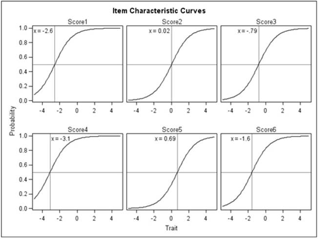
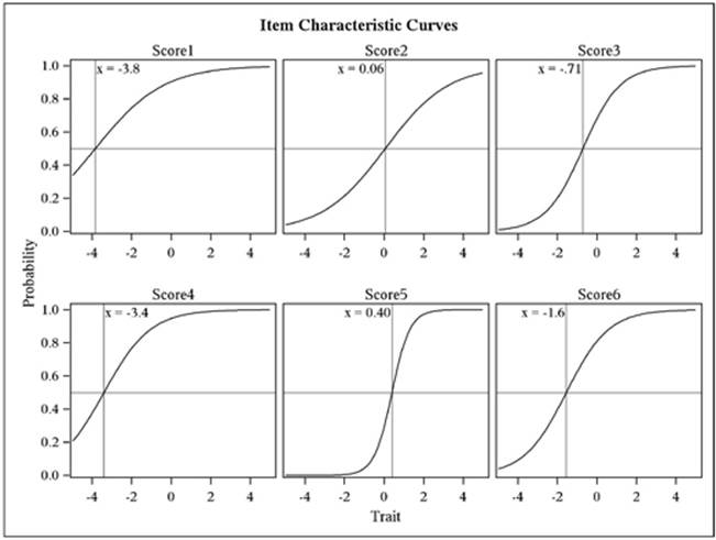
The most fundamental thing that we might look at in IRT is called an item characteristic curve (ICC). It is a model of the relationship between how much ability a person has on the trait being measured and how likely they are to get a particular item correct. With the Rasch, or 1PL model, the only thing we need to know about an item in order to get a model of this curve is the item difficulty. The Rasch model requires that all curves have roughly the same slope and that guessing isn’t a factor. The curve is a logistic ogive, and six of them are presented in Figure 8.1

You can see that the shape for these curves is identical but that they have been moved to the left or right, depending on how difficult the item was. The ability of persons is on the X axis on this graph, and the likelihood (probability) of getting the item right is on the Y axis. The scale on the X axis looks kind of like z-scores, but it could be transformed into any set of numbers. Item 4 (Score 4 in the figure) is the easiest of the six items. You can see that if a person’s ability was at 1.0, the probability of getting the item correct is in the high .90s. Item 5 is the most difficult item. Here a person with an ability of 1.0 would only have about a .60 chance of getting the item correct.

Now, you might be asking, "Geez, how did the data get to be so smooth for these graphs? Do test items really look like that?" The short answer is "No." These aren’t actual graphs of data, not even of smoothed data. They are curves of fixed characteristics that are laid in at the difficulty levels determined by the data. Now, since this is a set of graphs for dichotomously scored data (right = 1, wrong = 0), if we plotted all people in the data set individually, they would all have a Y value of 1 or 0. But if we grouped people into, say, six ability groups, we could get a better idea of whether the data for a given item really looks like the graphs presented below. If you think about it, for each of those observed data points, we would also have an expectation (given by the item characteristic curve), which would allow for a kind of chi-square analysis of fit. And that is what happens in IRT analysis, although again at a level of sophistication we can’t get into here.

We might get one more useful idea out of the graphs of Figure 8.1. Imagine that we gave these six items to an examinee and that person got three of them correct. What would we estimate that person’s ability to be? All we have to do is take an imaginary ruler, and move it from left to right on each of these items at the same time. If we stop that ruler at an estimate of -2.0, how many items would a person with that ability be expected to get right? To figure that out, we just have to go up the ruler to where it intersects with the curve and then read off the probability of getting that item right. For item 1, it looks like a person with an ability of -2.0 would have about a .55 chance of getting that item right. And then on item 2, the probability would be about .10, and then about .15 for item 3, etc. We could just add those probabilities together and find out, on average, how well we would expect a person with an ability of -2.0 to do on these six items together. To find out the ability of a person who got three items right, we just keep sliding the ruler to the right until the sum of the probabilities equals 3.0. It’s that simple.

With the 2PL and 3PL models, the slopes of these curves can vary from one ICC to the next, and the lower asymptote (where the curve stretches out to the left) can be greater than 0 if guessing is involved.

What We Aren’t Looking At!

IRT theory started with items that were scored dichotomously (right or wrong) and that only involved a single latent trait or ability. The theory has advanced dramatically over the years to be able to handle polytomous items (items scored on a scale) and multiple traits. These advances are both interesting and very useful but well beyond what we can address here.

Item Characteristics Curves from a One-Parameter Model

We now move on to how to use PROC IRT to analyze test data.

Preparing the Data Set for PROC IRT

In its simplest form, PROC IRT can model a series of dichotomous items with a unidimensional model. Program 8.1 below demonstrates how to run PROC IRT on the 56-item biostatistics test that was used to demonstrate classical item analysis in Chapter 5.

Program 8.1: Running PROC IRT for a Simple Binary Model

*Program 8.1;

*Preparing the stat test data set for PROC IRT;

data Binary;

infile 'c:\books\test scoring\stat_test.txt' pad;

array ans[56] $ 1 Ans1-Ans56; ***student answers;

array key[56] $ 1 Key1-Key56; ***answer key;

array score[56] Score1-Score56; ***score array 1=right,0=wrong;

retain Key1-Key56;

if _n_ = 1 then input @11 (Key1-Key56)($1.);

input @11 (Ans1-Ans56)($1.);

do Item=1 to 56;

Score[Item] = Key[Item] eq Ans[Item];

end;

keep Score1-Score56;

run;

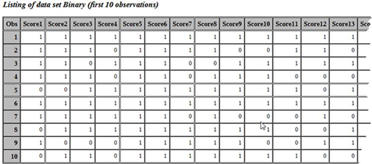
title "Listing of data set Binary (first 10 observations)";

proc print data=binary(obs=10);

run;

You start out by reading the answer key and the student answers as in previous programs. Here, however, there is no need to read the student IDs because PROC IRT is only looking for a set of binary (0/1) variables that represent, for each student, if an item was answered correctly (1) or incorrectly (0). You score the test in the usual way and keep the 56 Score variables.

Here are the first few observations in data set BINARY:

Running PROC IRT

The next step is to run PROC IRT as follows:

Program 8.2: Running PROC IRT (with All the Defaults)

*Program 8.2;

*Running PROC IRT (Unidimensional Model);

ods graphics on;

proc irt data=Binary;

var Score1-Score56;

run;

When you run this program, you will see the following error message in the SAS Log:

134

135 *Program 8.2;

136 *Running PROC IRT (Unidimensional Model);

137 ods graphics on;

138 proc irt data=Binary;

139 var Score1-Score56;

140 run;

ERROR: The number of levels for variable Score42 is smaller than 2.

NOTE: PROCEDURE IRT used (Total process time):

real time 0.06 seconds

cpu time 0.06 seconds

What went wrong? The error message is telling you that variable Score42 has fewer than two levels. This means that Score42 is all 0s (all students answered the item incorrectly) or all 1s (all students answered the item correctly – a more likely outcome). To be sure, you can run PROC FREQ as demonstrated in Program 8.3.

Program 8.3: Running PROC FREQ to Inspect Variable Score42

*Program 8.3;

*Identifying the Problem with Item 42;

title "Identifying the Problem with Item 42";

proc freq data=binary;

tables Score42 / nocum nopercent;

run;

Output from PROC FREQ follows:

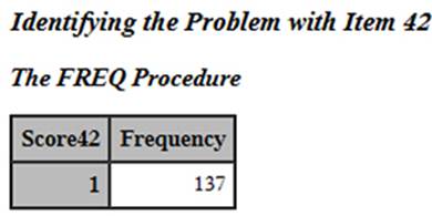
As you can see, your guess that all the students answered item 42 correctly is confirmed. The statistical methods used to create test models (in this case, a unidimensional model) require that each variable must have two levels. You need to run PROC IRT with Score42 removed from the variable list, as shown next.

Program 8.4: Running PROC IRT with Score42 Omitted

*Program 8.4;

*Running PROC IRT with Item 42 Removed;

ods graphics on;

title "PROC IRT with Item 42 Removed";

proc irt data=Binary plots=(scree(unpack) icc);

var Score1-Score41 Score43-Score56;

run;

In order to display some of the graphical output produced by PROC IRT, you need to do two things. First, you turn on ODS graphics (in versions of SAS 9.4 and higher, ODS graphics is turned on as the default and the ODS graphics statement is unnecessary). Second, you use a PLOTS= procedure option to request a scree plot (the UNPACK option places each of the two scree plots in a separate panel, rather than the two together) and an item characteristic curve (option ICC) for each item. Please note that even with relatively small tests taken by a few hundred students, this program may take considerable CPU time. For the sake of simplicity, we are shifting our analysis at this point to a 30-item physics test where we have a sample size of 102. Run Program 8.5, shown below, to run this model:

Program 8.5: Running a 1PL Model for a 30-Item Physics Test

title IRT Model on Physics Post Test;

proc irt data=test.all_post plots=(scree(unpack) icc);

var Score1-Score30;

model Score1-Score30;

run;

Here is the text portion of the output (broken down by sections):

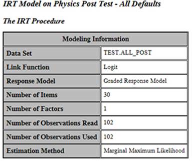
The modeling information presented here is simply a summary of what you’ve asked the program to do. Here we have 30 items and 102 people, and we’re using maximum likelihood estimation. The next part of the output shows item information:

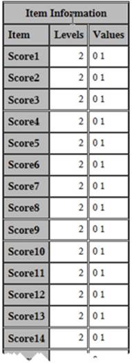
Because PROC IRT can be used for ordinal variables as well as binary ones, this section of output is included. With values of 0 or 1 for each item in this example, this portion of the output holds little interest.

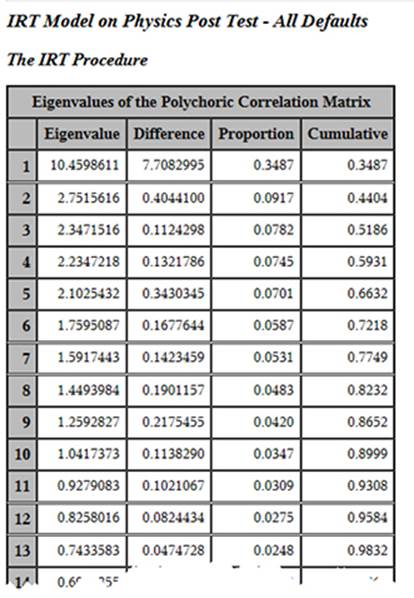
The first thing the program does is to run a factor analysis (principal components analysis) of the data to see if the underlying notion of a single trait being measured appears to be supported by the data. To check for this, we look at the eigenvalues. What you basically want to see here is the first eigenvalue being a lot larger than the second one. Then you want to see the third, fourth, etc., eigenvalues trailing off gradually after the second one. This indicates that you have a very strong first factor and that the remaining ones are pretty much indistinguishable. That appears to be the case in this situation. The first column is the eigenvalue itself, the second column is the difference between that eigenvalue and the next one (so for factor number one, we see that 10.4599 – 2.7516 = 7.7083). The third column tells you the proportion of the overall variance of the test items that is explained by that factor (10.4599/30 = 0.3487), and the last column gives you the cumulative proportion of variance that has been accounted for by that factor and the ones before it. Here we see a first eigenvalue that is four times larger than the second one, and the subsequent eigenvalues trail off gradually from the second one.

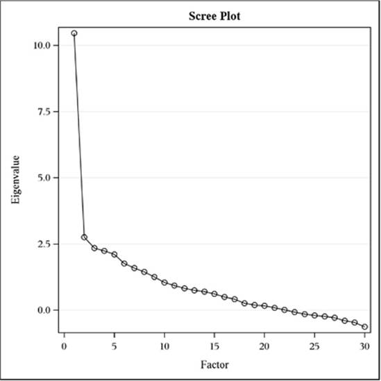
In some literature, you will see an argument for an eigenvalue greater than one criterion for how many factors there are in a data set. The logic there is that a factor should account for at least as much variance as an individual variable (or item) that comprises the factor analysis. But that criterion is way too liberal when a large number of variables (items) are in the factor analysis. A much better approach is called the scree plot approach. A scree plot is presented in Figure 8.2. It is a very simple plotting of the number of the eigenvalue (the first one, then the second one, etc.) on the X axis and the value of the eigenvalue on the Y axis. Thus, drawing from the table above, we see that the value in the scree plot for the first eigenvalue is 10.46, for the second one it’s 2.75, and so on. A quick visual inspection of this plot shows that the first eigenvalue is substantially higher than any of the subsequent eigenvalues and that eigenvalues 2 through 30 just gradually reduce.

What we learn from looking at the scree plot is that the test items from the physics test under consideration have a strong first factor and that proceeding with the IRT analysis seems a good idea.

Scree Plot Showing the Eigenvalues for Each Factor

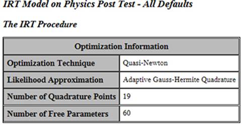
The next part of the analysis shows details on how the parameters for the analysis were estimated. Quasi-Newton and adaptive Gauss-Hermite Quadrature approaches each have their own Wikipedia pages; knock yourself out.

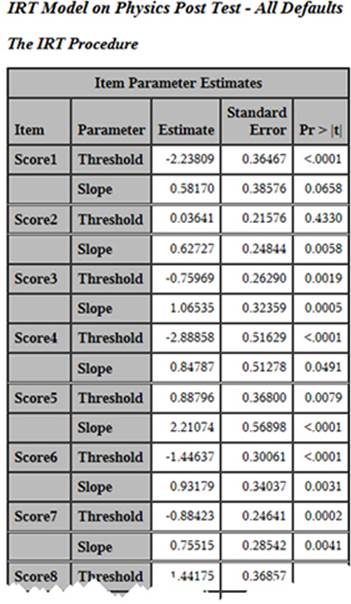
We now turn to the heart of the matter in looking at the output from the analysis. We have selected a 1PL model, which is basically the same idea as a Rasch analysis. The table above presents the item parameter estimates, which are essentially the critical pieces of information. In the table, we see columns for Item, Parameter, Estimate, Standard Error, and Pr > |t|. Item is the name we’ve given to the item, and Parameter tells us which parameter we are looking at for that item. (By "stacking" them, the program saves space horizontally.) Then we see the estimates, which are what we are after. For Score1, the threshold is -2.238 and the slope is 0.582. The numbering system for the threshold estimates are similar to z-scores. They run positive and negative and usually stay within +/-3.0. Although they are often a bit more spread out than z-scores, thez-score is not a bad analogy here. The slope is the slope of the relationship between ability and likelihood of a correct answer. The threshold is the point at which the probability of a correct answer would be .50 if the slope of the curve were equal to 1.0 (as it is assumed to be in the Rasch model). In the graphs shown below, the x value presented is the threshold divided by the slope, which provides the .50 level if the slope is assumed to be what the estimate says it is.

Some of the most interesting portions of the output are produced by ODS graphics. You see an item characteristic curve for each item on the test. If you look back at the output from Program 5.11 in Chapter 5, you see, at the far right, the proportion correct by quartile. If you plotted these values on the Y axis with the quartile values on the X axis, you would have a crude item characteristic curve. What PROC IRT does is model this curve from the test data and display it for you. Below are the item characteristic curves for the first six items. You need to keep in mind that these are idealized curves. The actual data will be much rougher in appearance than these curves.

Running Other Models

To run other models, such as a Rasch, 2PL, or 3PL, you need to add a MODEL statement and specify the model you wish to run as an option. For example, to run a Rasch model with the 30-item physics test data, you proceed as follows:

Program 8.6: Running a Rasch Model on the 30-Item Physics Test

title IRT Model on Physics Post Test - Rasch Model;

proc irt data=test.all_post plots=(scree(unpack) icc);

var Score1-Score30;

model Score1-Score30 / resfunc=rasch;

run;

You use the RESFUNC= (response function) option to specify that you want to run a Rasch model. Other model options that can be specified with PROC IRT are:

ONEP - specifies the one-parameter model.

TWOP - specifies the two-parameter model.

THREEP - specifies the three-parameter model.

FOURP - specifies the four-parameter model.

GRADED - specifies the graded response model.

RASCH - specifies the Rasch model.

There are many other options, such as the rotation method for your factor analysis, that you can specify with PROC IRT. The SAS help facility provides a list of these options along with several examples.

Classical Item Analysis on the 30-Item Physics Test

Before we conclude this chapter, we thought you might be interested in seeing the results from running a classical item analysis on the physics test data. Macros from Chapter 11 were used to score the physics test and produce the item analysis output. A portion of the output showing the analysis on the first 15 items is shown next:

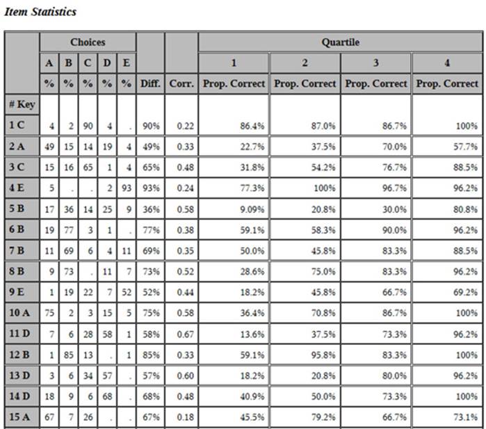
You see that item 1 was quite easy (90% of the students got it right) and item 2 was quite difficult (49% of the students got it right). This agrees with the threshold values in the IRT analysis, where the value for item 1 was -2.23809 and the threshold value for item 2 was.03641. That is, a low threshold indicates an easier item than a higher threshold. Take a look at the proportion correct by quartile and the point-biserial correlation for item 3. From a classical viewpoint, this is an excellent item. If you plotted the four proportion correct by quartile values (31.8%, 54.2%, 76.7%, and 88.5%), the resulting plot would have a similarity to the ICC curve produced by the IRT model. Seeing the IRT and classical output makes clear the two distinct purposes of these two methods of analysis—classical analysis is most useful for making decisions about individual items on a single test; IRT analysis is useful for calibrating items for item banks that will be used to assess student ability.

Conclusion

IRT is a fairly complicated approach to item analysis and test construction, and we have barely scratched the surface here. Our goal has been to provide an introduction to the analyses that SAS produces for IRT and to show how to run the procedure. To fully use IRT appropriately, you will need to consult the references listed (or similar ones) to develop a real sense of what IRT is about.

References

Baker, F. B. 2001. The basics of item response theory. ERIC Clearinghouse on Assessment and Evaluation. Retrieved 4/20/2014: http://echo.edres.org:8080/irt/baker/final.pdf

DeMars, C. 2010. Item Response Theory. Oxford: Oxford University Press.

Hambleton, R. K., Swaminathan, H., & Rogers, H. J. 1991. Fundamentals of Item Response Theory. Newbury Park, CA: Sage Press.

Lord, F. M. 1980. Applications of item response theory to practical testing problems. Mahwah, NJ: Lawrence Erlbaum Associates.

Rasch, G. 1961. On general laws and the meaning of measurement in psychology. In Proceedings of the fourth Berkeley symposium on mathematical statistics and probability (Vol. 4, pp. 321-333). Berkeley, CA: University of California Press.

Wright, B. D. 1977. Solving measurement problems with the Rasch model. Journal of Educational Measurement, 14(2), 97-116.