Excel VBA 24-Hour Trainer (2015)

Part III
Beyond the Macro Recorder: Writing Your Own Code

Lesson 11
Programming Formulas

Spreadsheets are a popular choice for managing information because mathematical calculations and data analysis are, and always will be, a requirement of education, business, and personal record-keeping. If there were no need to compile numeric data with formulas, there'd be no need for spreadsheets as we know them—an unfathomable thought in our information-ravenous, digital world.

As you've seen, VBA enables you to programmatically manipulate Excel's objects, methods, and properties. You can interact with users to make decisions and establish conditions. Just as importantly, you need to understand how to program formulas, starting with how Excel regards locations of cells and ranges by their row and column references.

Understanding A1 and R1C1 References

Most people who use Excel—most being around 99.9 percent—view Excel worksheets with rows headed from the top as numbers 1, 2, 3 and continuing downward, and columns headed from the left as letters A, B, C and continuing to the right. The top-left cell address on the Excel grid is commonly seen as cell A1. The cell immediately below A1 is A2, the cell to the right of A2 is B2, and so on.

Behind the scenes, Excel does not refer to its rows and columns in A1 style; that is, not in the sequence of column letter and row number. Rather, Excel regards rows and columns as numbers, in R1C1 style, expressing a cell address in the sequence of its intersecting row number and column number.

NOTE If you are wondering if understanding R1C1 style is really important enough to stay with this lesson, the answer is yes, it really is important enough. As concepts go, understanding R1C1 style gives you the most bang for your buck in terms of the long-term benefit you get from spending the few minutes to read this lesson. Your VBA programming skills will advance much faster and easier once you get a handle on R1C1 references.

In R1C1 style, “R” stands for row and “C” stands for column. For example, cell D7 is identified by Excel as the address at the intersection of row 7 and column 4 (because column D is the fourth column from the left on the worksheet grid), which Excel interprets as R7C4. Cell M92 is interpreted as R92C13, and so on. As you might guess, the R1C1 address of cell A1 is R1C1.

Getting Started with a Few One-Liners

As you will see on the following pages, R1C1 cell references do not always look as clean as just a number for a row and a number for a column. The R1C1 style uses a starting reference point, and without one specified, assumes cell A1 as the default reference. For example, suppose your active cell is H22. To refer to a cell 3 rows up and 5 columns to the right, which is cell M19, then with cell H22 as the reference point (that is, as far as cell H22 is concerned), cell M19 would be referred to as =R[-3]C[5].

NOTE You can plug the following four examples of single code lines into a macro, or you can quickly execute them in the Immediate window. You may recall from Lesson 3 that you can access the Immediate window easily by pressing Alt+F11 to go to the Visual Basic Editor, then pressing Ctrl+G to enter the Immediate window. Just copy and paste any of these single code lines into the Immediate window and press Enter. To see the results, press Alt+Q to return to the worksheet.

To enter a formula programmatically in cell H22 that shows the value in cell M19, your line of code would be this, using a relative reference to cell M19:

Range("H22").FormulaR1C1 = "=R[-3]C[5]"

As another example, if you want the formula in cell H22 to return the value in cell H26, which is 4 rows greater than row number 22 and in the same column H, that code line would be as follows:

Range("H22").FormulaR1C1 = "=R[4]C"

If you want the formula in cell H22 to return the value in cell A22, which is on the same row but 7 columns less than column number 8 (Excel and VBA regard column H as column 8), that code line would be:

Range("H22").FormulaR1C1 = "=RC[-7]"

Finally, if you want to enter a formula in cell H22, or any cell for that matter, to return the value in cell F3, such that the formula's row and column references are absolute (making the formula look like =$F$3), this line of code would do that:

Range("H22").FormulaR1C1 = "=R3C6"

NOTE You have probably noticed that Excel and VBA rarely regard cell addresses by column letter and row number. It can be a challenge at first to stray from the familiar thought process of referencing cell addresses in A1 style, considering the alpha column headers and worksheet formulas that are almost always how worksheets are viewed. Recall from Lesson 8 that the Cellsproperty refers to addresses in R1C1 style, by their row number and column number. For example, the statement Cells(5, 2).Select would select cell B5 of the active worksheet, which is a syntax you have already seen. The more you work with VBA, the more you will see how useful the R1C1 style is, and how limiting the A1 style will be.

Comparing the Interface of A1 and R1C1 Styles

It's been said that a picture is worth a thousand words. Take a look at the next several figures to see worksheets from an R1C1 point of view. The comparison figures help you to see formulas and worksheets the way Excel and VBA sees them.

NOTE There's a pro-R1C1 tone to this chapter, but I'm not suggesting you change your worksheet viewing habits to the R1C1 view if you've been working in A1 view. In fact, I always work in A1 view, just as most Excel users do. The goal in this chapter is to explain what R1C1 is and how it works.

Figure 11.1 shows a side-by-side comparison of A1 and R1C1 styles for the same spreadsheet. Notice the active cell address in the name box, the column headers, and the formula as displayed in the formula bar vary between the two styles.

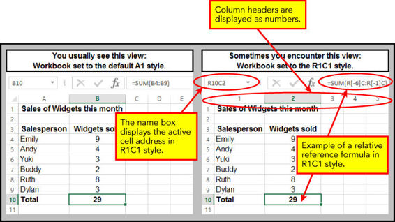
Figure 11.1

Toggling between A1 and R1C1 Style Views

Occasionally on Excel forums, or in e-mails I receive from people who follow my work, the question comes up about how and why their worksheets inexplicably show column headers as numbers. The reason is that someone unwittingly changed the view in that workbook from A1 to R1C1 style, and forgot how to undo the mysterious deed.

NOTE Your workbook doesn't need to be in R1C1 style to use .FormulaR1C1 in your code. This is just an exercise to show how to get in and out of R1C1 style, and what that style looks like.

Here's how to toggle between the two views. Start by clicking the File tab so that you go to the backstage view. Click the Options item on the vertical menu, as shown in Figure 11.2 when using Excel version 2013.

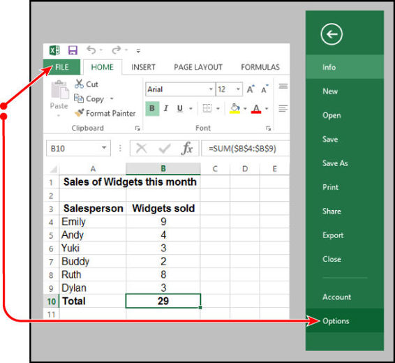
Figure 11.2

In the Excel Options dialog box, click the Formulas item in the menu pane at the left. Select the check box for R1C1 Reference Style in the Working with Formulas section, and click OK, as shown in Figure 11.3.

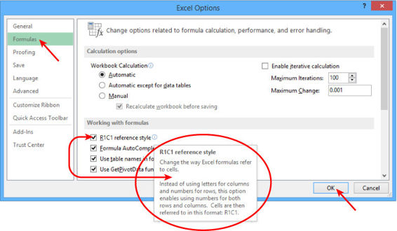
Figure 11.3

If you are using Excel 2003, click the Tools item on the menu bar, and select Options, as shown in Figure 11.4. In the Options dialog box, click the General tab, select R1C1 Reference Style in the Settings section, and click OK, as shown in Figure 11.5.

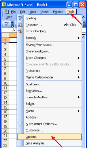
Figure 11.4

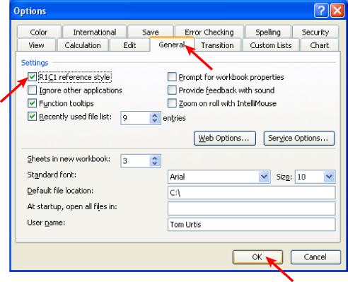
Figure 11.5

Here's another comparison of the two styles side by side. Figure 11.6 shows an example of an absolute reference formula in cell B10 (or if you prefer, in cell R10C2). To return to A1 style, simply repeat the preceding steps and deselect the option for R1C1 Reference Style.

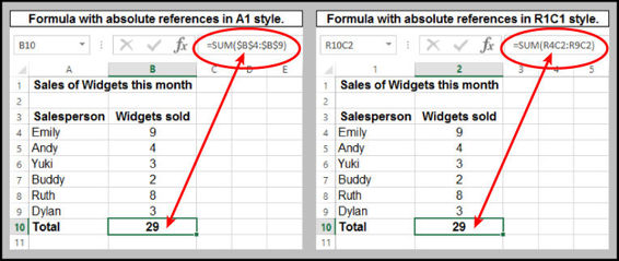
Figure 11.6

Programming Your Formula Solutions with VBA

The following examples can give you some insight for designing formulas in macros to solve common situations. With VBA you can include variable names and named ranges in your formulas, providing creative ways to get your work done.

NOTE If and when you use the Macro Recorder to produce formulas to plug into your macros, you'll notice that formulas are recorded in R1C1 style, in whichever style you are in.

Using a Mixed Reference to Fill Empty Cells with the Value from Above

Figure 11.7 shows a before-and-after look at how you can use a mixed reference formula (as shown in the following snippet) to fill empty cells with the preceding constant value. Using the SpecialCells property, the same formula is entered into every blank cell in column A that is associated with the list:

Sub FillBlankCellsFromAbove()

Application.ScreenUpdating = False

With Columns(1)

.SpecialCells(xlCellTypeBlanks).Formula = "=R[-1]C"

'Convert formulas into static values.

.Value = .Value

End With

Application.ScreenUpdating = True

End Sub

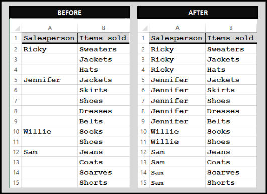
Figure 11.7

NOTE With Columns(1) refers to column A. If you were working with column H, you would have written the code as With Columns(8).

Using a Named Range with Relative, Mixed, and Absolute References

This example shows how to deal with several issues you might encounter. In 11.8, a payroll worksheet needs a conditional formula in range D5:D12 to calculate the weekly salaries for each employee. Eligibility for overtime pay is based on the criteria of 40 maximum regular hours in cell B1. The overtime multiplication factor in cell B2 is the named range OvertimeFactor, which is multiplied for each hour past the 40-hour ceiling.

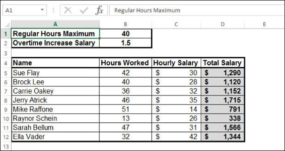
Figure 11.8

The formula in cell D5 and copied to cell D12 is =IF(B5<=$B$1,B5*C5,SUM((B5-$B$1) *OvertimeFactor,$B$1)*C5), which you can see in the formula bar in Figure 11.9. In the following macro, notice the syntax for relative, mixed, and absolute references, along with the inclusion of a named range, the If statement, and a nested SUM function:

Sub CalculateSalary()

Range("D5:D12").FormulaR1C1 = _

"=IF(RC[-2]<=R1C2,RC[-2]*RC[-1],SUM((RC[-2]-R1C2)*OvertimeFactor,R1C2)*RC[-1])"

End Sub

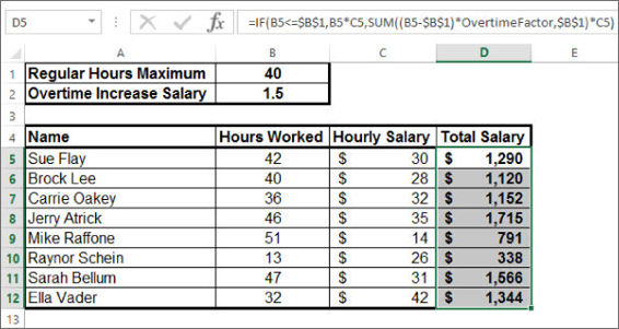
Figure 11.9

Programming an Array Formula

As you know, when you compose an array formula manually, you must commit it to a worksheet cell by pressing the Ctrl+Shift+Enter keys, not just the Enter key. Similarly, when you want to install an array formula programmatically, you must use the FormulaArray method, not just the Formula or Formula R1C1 methods. The FormulaArray method is VBA's way of differentiating between an array and a non-array formula.

In Figure 11.10, array formulas are entered into destination cells B19, B20, and B21 with the following macro that averages scores for each of three lanes at a bowling alley. For a bit of variety to show an alternative cell reference syntax, I looped through each of the three destination cells (where the array formulas will go) using the Range statement that shows column letter B followed by the row numbers represented by a Long type variable named lngRow:

Sub AverageBowlingScores()

Dim lngRow As Long

For lngRow = 19 To 21

Range("B" & lngRow).FormulaArray = _

"=AVERAGE(IF(R4C1:R16C1=RC[-1],R4C3:R16C6))"

Next lngRow

End Sub

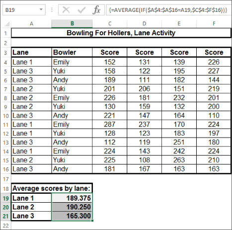
Figure 11.10

WARNING When you have a lot of formulas on a worksheet for which you want to convert all cell and range references from relative to absolute, this macro can do the job:

Sub ConvertRelativeToAbsolute()

Dim cell As Range, strFormulaOld As String, strFormulaNew As String

For Each cell In Cells.SpecialCells(xlCellTypeFormulas)

strFormulaOld = cell.Formula

strFormulaNew = _

Application.ConvertFormula _

(Formula:=strFormulaOld, fromReferenceStyle:=xlA1, _

toReferenceStyle:=xlA1, toAbsolute:=xlAbsolute)

cell.Formula = strFormulaNew

Next cell

End Sub

And here's how you can convert absolute reference formulas to relative references on a worksheet:

Sub ConvertAbsoluteToRelative()

Dim cell As Range, strFormulaOld As String, strFormulaNew As String

For Each cell In Cells.SpecialCells(xlCellTypeFormulas)

strFormulaOld = cell.Formula

strFormulaNew = _

Application.ConvertFormula _

(Formula:=strFormulaOld, fromReferenceStyle:=xlA1, _

toReferenceStyle:=xlA1, toAbsolute:=xlAbsolute)

cell.Formula = WorksheetFunction.Substitute(strFormulaNew, "$", "")

Next cell

End Sub

NOTE Here's a quick way to count your workbook's formulas, and show the total count in a message box subtotaled by worksheet name. The statements On Error Resume Next, Err.Number, andErr.Clear help to bypass potential stoppages of the macro, known as runtime errors, if (in this example) a worksheet does not contain any formulas. In Lesson 20, you become familiar with these and other error-related terms, along with techniques for handling errors in your code.

Sub CountFormulas()

Dim SheetFormulaCount As Long, TotalFormulaCount As Long

Dim myList As String, WS As Worksheet

SheetFormulaCount = 0: TotalFormulaCount = 0: myList = ""

For Each WS In Worksheets

'optional if your sheets are protected

'WS.Unprotect ("YourPassword")

On Error Resume Next

SheetFormulaCount = WS.Cells.SpecialCells(xlCellTypeFormulas).Count

If Err.Number <> 0 Then

Err.Clear

SheetFormulaCount = 0

End If

TotalFormulaCount = TotalFormulaCount + SheetFormulaCount

myList = myList & "Formula count in ''" & WS.Name & "'': " & _

Format(SheetFormulaCount, "#,##0") & vbCrLf

'optional reprotect your sheets

'WS.Protect ("YourPassword")

Next WS

MsgBox myList & vbCrLf & "Total formulas in " & _

ThisWorkbook.Name & ": " & _

Format(TotalFormulaCount, "#,##0"), , "Workbook formula count"

End Sub

Summing Lists of Different Sizes along a Single Row

In Figure 11.11, a table has several columns, each containing a varying count of numeric entries needing to be summed. When you want to show the sums of each column along a single row, you first need to identify the last used row among all the columns, and install your sum formulas in the next row below that. The idea is to place the sums for each column in the first available row that has no data in any column.

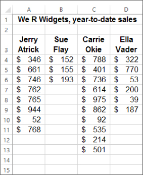
Figure 11.11

In Figure 11.11, the last used row is 13 because column C contains entries that extend to cell C13. Tomorrow, you might get a similar table, maybe with more columns, where the last used row will be 128 in column K. This is where VBA really shines when you program formulas in R1C1 style when dealing with dynamic ranges. No matter how many columns the table has, or which column has the most entries, the following macro named SumAlongOneRow sums each column's numbers along the first unused row. The result is shown in Figure 11.12.

Sub SumAlongOneRow()

'Declare and define a Long type variable for the next available row

'where all the SUM formulas will go.

Dim NextRow As Long

NextRow = _

Cells.Find(What:="*", After:=Range("A1"), _

SearchOrder:=xlByRows, SearchDirection:=xlPrevious).Row + 1

'Declare and define a Long type variable to identify the last column

'in the used range.

Dim LastColumn As Long

LastColumn = _

Cells.Find(What:="*", After:=Range("A1"), _

SearchOrder:=xlByColumns, SearchDirection:=xlPrevious).Column

'The used range starts in column A which is Column 1 in VBA.

'The sales numbers in the table start on row 4.

'Therefore, sum the numbers with a formula that starts at

'row 4 and ends at the last used row, which is one row above

'(numerically 1 less than) the last used row.

Range(Cells(NextRow, 1), Cells(NextRow, LastColumn)).FormulaR1C1 _

= "=SUM(R4C:R" & NextRow - 1 & "C)"

End Sub

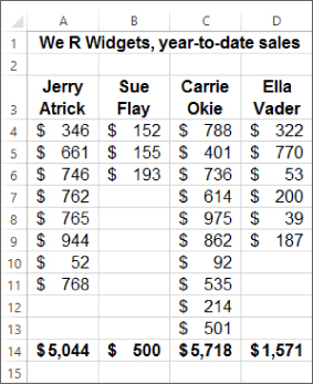
Figure 11.12

NOTE You probably know that the RAND worksheet function enters a random number in a cell. RAND is among a group of functions called volatile functions. Volatile functions recalculate whenever another cell in the workbook is changed, or some event takes place such as opening the workbook. You might want to enter a random number and keep it static—that is, for the random number to not change unless you want to change it again, if ever. You can enter a static random number using the following line of code, executable in the Immediate window or as part of a macro. This is an example of how to enter a static random number between 1 and 100 in cell A1. Notice that a value, not actually a formula, is being entered:

Range("A1").Value = Format(Rnd() * 99 + 1, "000")

Try It

For this lesson, you install formulas to sum the numbers in each column of a sales report table. Each column has a varying count of entries, and you want the sum formulas to be placed in the first empty cell below each column's last numeric entry.

Lesson Requirements

To get the sample workbook, you can download Lesson 11 from the book's website at www.wrox.com/go/excelvba24hour.

Step-by-Step

1. In your Excel workbook, press Alt+F11 to go to the Visual Basic Editor.

2. From the VBE menu bar, click Insert Module.

3. In the new module, type the name of your macro: SumEachColumnNextRow. Press Enter, and VBA automatically places a pair of parentheses after the macro name, followed by an empty line, followed by the End Sub statement. Your code looks as follows:

4. Sub SumEachColumnNextRow ()

End Sub

4. Declare a Long type variable to identify the last column in the used range, a Long type variable for the last row of numbers present in each column (below which each column's SUM formula will go), and a Longtype variable for the column numbers that will be looped through:

Dim LastColumn As Long, lngColumn As Long, LastRow As Long

5. Use the LastColumn variable inside a loop at each iteration:

6. LastColumn = Cells.Find(What:="*", After:=Range("A1"), _

SearchOrder:=xlByColumns, SearchDirection:=xlPrevious).Column

6. Loop through each column in the used range. The used range starts in column A, which VBA sees as column number 1. Loop through each column and install the formula in the first unused row. While you're at it, bold those sum formula cells to make them easier to see:

7. For lngColumn = 1 To LastColumn

8. LastRow = Cells(Rows.Count, lngColumn).End(xlUp).Row

9. With Cells(LastRow + 1, lngColumn)

10. .FormulaR1C1 = "=SUM(R4C:R" & LastRow & "C)"

11. .Font.Bold = True

12. End With

Next lngColumn

7. Press Alt+Q to return to the worksheet and test your macro. After you run the macro, the result looks like Figure 11.13. Here's the macro named SumEachColumnNextRow in its entirety:

8. Sub SumEachColumnNextRow()

9. 'Declare a Long type variable to identify the last column

10. 'in the used range.

11. 'Declare a Long type variable for the last row of numbers present

12. 'in each column, below which each column's SUM formula will go.

13. 'Declare a Long type variable for the column numbers that

14. 'will be looped through.

15. Dim LastColumn As Long, lngColumn As Long, LastRow As Long

16. 'You will use this variable in a loop at each iteration.

17. LastColumn = _

18. Cells.Find(What:="*", After:=Range("A1"), _

19. SearchOrder:=xlByColumns, SearchDirection:=xlPrevious).Column

20. 'Loop through each column in the used range.

21. 'The used range starts in column A which is Column 1 in VBA.

22. 'Loop through each column and install the formula in the first

23. 'unused row. While we are at it, bold those sum formula cells

24. 'to make them easier to see.

25. For lngColumn = 1 To LastColumn

26. LastRow = Cells(Rows.Count, lngColumn).End(xlUp).Row

27. With Cells(LastRow + 1, lngColumn)

28. .FormulaR1C1 = "=SUM(R4C:R" & LastRow & "C)"

29. .Font.Bold = True

30. End With

31. Next lngColumn

End Sub

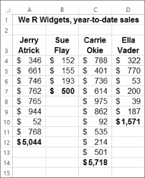
Figure 11.13

REFERENCE Please select the videos for Lesson 11 online at www.wrox.com/go/excelvba24hour. You will also be able to download the code and resources for this lesson from the website.