Excel VBA 24-Hour Trainer (2015)

Part III
Beyond the Macro Recorder: Writing Your Own Code

Lesson 15
Handling Duplicate Items and Records

When you work with data in tables or lists, it is common for some items to appear more than once. Two situations usually arise when duplicate items exist, depending on the nature of the work at hand:

· The repeated items are unwanted and need to be deleted. For example, if you are compiling a list of e-mail addresses, or you are gathering a list of people's names for invitation to an event, you would only want a list of unique items.

· Items are expected to be repeated in the list and need to be maintained for analysis or record-keeping. For example, a list of monthly payments made to a vendor would show that vendor's name with each transaction.

Deleting Rows Containing Duplicate Entries

Suppose a table of data contains duplicate items in one or more columns. To delete rows containing duplicate items, the first step is to determine if the table contains duplicates in just one column, or if several (maybe all) columns contain duplicate data.

Deleting Rows with Duplicates in a Single Column

Suppose you have a list of items that are repeated in column A. The macro named DeleteDupesColumnA uses AdvancedFilter to expose the first instance of every item in column A. The exposed rows are marked with a value (the numeral 1 in this example, but it could be any value) in a helper column. All rows with empty cells in the helper column are deleted.

NOTE For my money, AdvancedFilter is the second-most powerful tool in Excel, behind pivot tables. One of AdvancedFilter's capabilities is to filter for unique items in a large list at lightning speed.

The macro executes in the blink of an eye, even for a list with tens of thousands of rows. There are comments at each step to explain the deletion process using AdvancedFilter:

Sub DeleteDupesColumnA()

'Long variable for last used column.

Dim LastColumn As Long

With Application

.ScreenUpdating = False

'Determine last column number of table, and add a 1 to it

'to establish a helper column that is the column after

'the last column in the data table.

LastColumn = _

Cells.Find(What:="*", After:=Range("A1"), SearchOrder:=xlByColumns, _

SearchDirection:=xlPrevious).Column + 1

'AdvancedFilter exposes unique entries and enters a 1 in the helper

'column on the same row of items that first appear in the list.

With Range("A1:A" & Cells(Rows.Count, 1).End(xlUp).Row)

.AdvancedFilter Action:=xlFilterInPlace, Unique:=True

.SpecialCells(xlCellTypeVisible).Offset(0, LastColumn - 1).Value = 1

'Error bypass that is explained in Lesson 20.

'This is to avoid the macro stopping if no duplicate values existed.

On Error Resume Next

'Show all rows by exiting AdvancedFilter.

ActiveSheet.ShowAllData

'Delete rows where empty cells exist in the helper column,

'indicating that the value in column A is a duplicate.

Columns(LastColumn).SpecialCells(xlCellTypeBlanks).EntireRow.Delete

Err.Clear

End With

'Clear the helper column.

Columns(LastColumn).Clear

.ScreenUpdating = True

End With

End Sub

Your lists will not always have its duplicate entries in column A. The next list you receive might have its duplicate entries in a different column, say column D. The DeleteDupesColumnD macro is a modification of the previous macro, with comments showing where and how to change the relevant column references:

Sub DeleteDupesColumnD()

'Ask the user to confirm their intention of deleting

'the duplicate items in column D.

Dim myConfirmation As Integer

myConfirmation = _

MsgBox("Do you want to delete the duplicates" & vbCrLf & _

"in column D?" & vbCrLf & vbCrLf & _

"Once the duplicates are deleted," & vbCrLf & _

"the macro cannot undo that action.", _

vbQuestion + vbYesNo, _

"Please confirm:")

'If the answer is no, exit the macro.

If myConfirmation = vbNo Then

MsgBox "That's fine, nothing will be deleted.", _

vbInformation, _

"You clicked No."

Exit Sub

Else

'If the answer is yes, continue with the deletion.

MsgBox "Please click OK to delete the duplicates.", _

vbInformation, _

"Thanks for confirming!"

End If

With Application

.ScreenUpdating = False

Dim LastColumn As Long

LastColumn = _

Cells.Find(What:="*", After:=Range("A1"), SearchOrder:=xlByColumns, _

SearchDirection:=xlPrevious).Column + 1

'In the next line you specify column D.

'If this were for column L instead of column D, the code would read

'With Range("L1:L" & Cells(Rows.Count, 12).End(xlUp).Row)

With Range("D1:D" & Cells(Rows.Count, 4).End(xlUp).Row)

.AdvancedFilter Action:=xlFilterInPlace, Unique:=True

'In the next line, notice the number 4 in the Cells property,

'which is column D. If this were for column L instead of column D,

'number 4 would be 12, example .Offset(0, LastColumn - 12).Value = 1

.SpecialCells(xlCellTypeVisible).Offset(0, LastColumn - 4).Value = 1

On Error Resume Next

ActiveSheet.ShowAllData

Columns(LastColumn).SpecialCells(xlCellTypeBlanks).EntireRow.Delete

Err.Clear

End With

Columns(LastColumn).Clear

.ScreenUpdating = True

End With

End Sub

NOTE Notice in these macros that no cell or row is selected, which would have slowed things down, and a filter is utilized for the entire range instead of a loop for each row. When deleting rows, use a filter when you can because it is much faster than looping through cells one by one.

Please keep in mind that there is not an undo option after a macro runs. It's a wise practice to let the users of your projects know the consequence of running a macro that deletes data. For example, the DeleteDupesColumnD macro begins with a message box to inform the user that the macro's actions cannot be undone, and to confirm their intention to delete the duplicate items.

Deleting Rows with Duplicates in More Than One Column

When you have a list of data, sometimes it is not enough to simply delete rows with duplicated information based only on the items in one column. Multicolumn lists can have duplicated records when every item in every column of a row's data matches that of another row's entire data. In those cases, you need to compare a concatenated string of each record's (row's) data, and compare that to the concatenated strings of all the other rows.

Take a close look at Figure 15.1. In the original list, every item in rows 5 and 7 match, as do all the items in rows 3 and 10. This is a short list for demonstration purposes. If your list were thousands of rows long, you would need a quick way to delete duplicate records. The macro named DeleteDuplicateRecords is one way to do the job, with comments at each step.

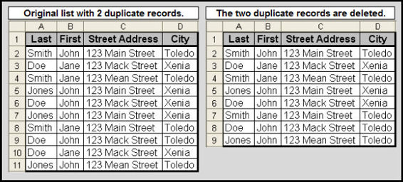
Figure 15.1

NOTE There is an error bypass method in some of these macros that might be unfamiliar to you. Lesson 20 covers the topic of error handling.

Sub DeleteDuplicateRecords()

'Turn off ScreenUpdating to speed up the macro.

Application.ScreenUpdating = False

'Declare a range variable for the helper column being used.

Dim FilterRange As Range

'Define the range variable's dynamic range.

Set FilterRange = Range("E1:E" & Cells(Rows.Count, 1).End(xlUp).Row)

'For efficiency, open a With structure for the FilterRange variable.

With FilterRange

'Enter the formula

'=SUMPRODUCT(($A$1:$A1=$A1)*($B$1:$B1=$B1)*($C$1:$C1=$C1)*($D$1:$D1=$D1))>1

'in all cells in column E (the helper column) that returns either TRUE

'if the record is a duplicate of a previous one, or FALSE if the record

'is unique among the records in all previous rows in the list.

.FormulaR1C1 = _

"=SUMPRODUCT((R1C1:RC1=RC1)*(R1C2:RC2=RC2)*(R1C3:RC3=RC3)*(R1C4:RC4=RC4))>1"

'Turn the formulas into static values because they will be filtered,

'and maybe deleted if any return TRUE.

.Value = .Value

'AutoFilter the helper column for TRUE.

.AutoFilter Field:=1, Criteria1:="TRUE"

'Error bypass in case no TRUEs exist in the helper column.

On Error Resume Next

'This next line resizes the FilterRange variable to exclude the first row.

'Then, it deletes all visible filtered rows.

.Offset(1).Resize(.Rows.Count - 1).SpecialCells(xlCellTypeVisible).EntireRow.Delete

'Clear the Error object in case a run time error would have occurred,

'that is, if no TRUEs existed in the helper column to be deleted.

Err.Clear

'Close the With structure for the FilterRange variable object.

End With

'Exit (stop using) AutoFilter.

ActiveSheet.AutoFilterMode = False

'Clear all helper values (there would only be FALSEs at this moment).

'Note that Columns(5) means column E which is the fifth column from the left

'on an Excel spreadsheet.

Columns(5).Clear

'Clear the range object variable to restore system memory.

Set FilterRange = Nothing

'Turn ScreenUpdating back on.

Application.ScreenUpdating = True

End Sub

Deleting Some Duplicates and Keeping Others

This section shows a “this way or that way” pair of macros that use an array to hold a set of items to determine which rows you want to keep or delete. In Figure 15.2, an original list has clothing items in column A that are accompanied by various colors of those items in column B.

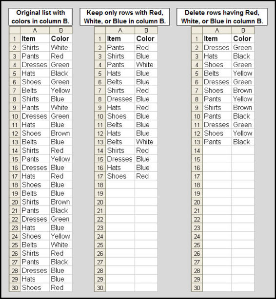
Figure 15.2

Both macros hold the same array items of Red, White, and Blue. The macro named KeepOnlyArrayColors keeps all rows where Red, White, or Blue are found in column B, while deleting all the other rows. The macro named DeleteArrayColors does the opposite: It deletes all rows where Red, White, or Blue are found in column B, but keeps all the other rows.

Sub KeepOnlyArrayColors()

Application.ScreenUpdating = False

Dim LastRow as Long, rng As Range

LastRow = Cells(Rows.Count, 1).End(xlUp).Row

Set rng = Range("B2:B" & LastRow)

Dim ColorList As Variant, ColorItem As Variant

ColorList = Array("Red", "White", "Blue")

For Each ColorItem In ColorList

rng.Replace What:=ColorItem, Replacement:=ColorItem & "|", LookAt:=xlWhole

Next ColorItem

rng.AutoFilter Field:=1, Criteria1:="<>*|"

On Error Resume Next

rng.SpecialCells(xlCellTypeVisible).EntireRow.Delete

Err.Clear

rng.Replace What:="|", Replacement:="", LookAt:=xlPart

Set rng = Nothing

ActiveSheet.AutoFilterMode = False

Application.ScreenUpdating = True

End Sub

Sub DeleteArrayColors()

Application.ScreenUpdating = False

Dim LastRow as Long, rng As Range

LastRow = Cells(Rows.Count, 1).End(xlUp).Row

Set rng = Range("B2:B" & LastRow)

Dim ColorList As Variant, ColorItem As Variant

ColorList = Array("Red", "White", "Blue")

For Each ColorItem In ColorList

rng.Replace What:=ColorItem, Replacement:="", LookAt:=xlWhole

Next ColorItem

On Error Resume Next

rng.SpecialCells(xlCellTypeBlanks).EntireRow.Delete

Err.Clear

Set rng = Nothing

Application.ScreenUpdating = True

End Sub

Working with Duplicate Data

As I wrote at the beginning of this lesson, the nature of some projects is to expect duplicated data and to work with it in some way. The following examples show how VBA can make duplicated data work to your advantage.

Compiling a Unique List from Multiple Columns

From a single-column list containing repeated items, you can extract a list of unique items using AdvancedFilter. For example, the following line of code copies a unique list of items from column A into column B:

Range("A1").CurrentRegion.AdvancedFilter Action:=xlFilterCopy, _

CopyToRange:=Range("B1"), Unique:=True

The question becomes, what if you want to extract a unique list from a table that has many columns of repeatedly listed items? In Figure 15.3, a fictional quarterly survey ranks the top-10 vacation destinations. Many of those destinations are repeated among the four quarterly columns. The macro named UniqueList lists all unique vacation destinations from the table in column G:

Sub UniqueList()

'Turn off ScreenUpdating

Application.ScreenUpdating = False

'Declare and define variables

Dim cell As Range, TableRange As Range

Dim xRow As Long, varCell As Variant

Set TableRange = Range("B4:E13")

xRow = 2

'Clear column G (column #7) where the unique list will go.

Columns(7).Clear

'Enter the header label in cell G1 and bold cell G1.

With Range("G1")

.Value = "Unique list:"

.Font.Bold = True

End With

'Loop through each cell in the table range,

'and add that cell's value to the list if it

'does not exist in the list yet.

For Each cell In TableRange

varCell = Application.Match(cell.Value, Columns(7), 0)

If IsError(varCell) Then

Err.Clear

Cells(xRow, 7).Value = cell.Value

xRow = xRow + 1

End If

Next cell

'Clear the TableRange object variable from system memory.

Set TableRange = Nothing

'Optional, sort the list in alphabetical order.

Range("G1").CurrentRegion.Sort Key1:=Range("G2"), _

Order1:=xlAscending, Header:=xlYes

'Autofit column G.

Columns(7).AutoFit

'Turn ScreenUpdating back on.

Application.ScreenUpdating = True

End Sub

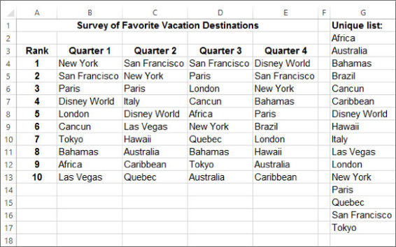
Figure 15.3

Updating a Comment to List Unique Items

This section shows how you can automatically update a comment to show unique items in sorted order from a list containing repeated items. When a new unique item is added to the list, the comment is immediately updated in real time.

In Figure 15.4, a company keeps an ongoing list of its clients and dates of transactions. When a new client is added to the list, such as what is happening in cell A20, the comment in cell A1 is updated to show that new client name in a sorted list.

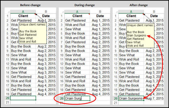
Figure 15.4

NOTE This example uses a Worksheet_Change event procedure. The code goes into the module of your worksheet. Lesson 13 covers event coding, including how and where to place this code.

Private Sub Worksheet_Change(ByVal Target As Range)

'Limit the event to monitor only changes in column A.

If Target.Column <> 1 Then Exit Sub

'Prepare Excel's application settings.

With Application

.ScreenUpdating = False

.DisplayAlerts = False

.EnableEvents = False

'Declare variables.

Dim HelperColumn As Long, cell As Range, strCommentText As String

'Define the helper column which is the last used column + 2,

'to use for listing the unique client names and sorting them.

HelperColumn = _

Cells.Find(What:="*", After:=Range("A1"), _

SearchOrder:=xlByColumns, _

SearchDirection:=xlPrevious).Column + 2

'List the unique client names in the helper column.

Range("A1:A" & Cells(Rows.Count, 1).End(xlUp).Row).AdvancedFilter _

Action:=xlFilterCopy, CopyToRange:=Cells(1, HelperColumn), Unique:=True

'Sort the unique client list in ascending order.

Cells(1, HelperColumn).Sort _

Key1:=Cells(2, HelperColumn), _

Order1:=xlAscending, _

Header:=xlYes

'Build the comment's text string, comprised by each unique client name

'in a vertical list. To do that, separate each name with the ascii 10

'carriage return character.

strCommentText = ""

For Each cell In Cells(1, HelperColumn).CurrentRegion

'Bypass the header cell in row 1.

If cell.Row <> 1 Then _

strCommentText = strCommentText & Chr(10) & cell.Value

Next cell

strCommentText = "Unique client names:" & Chr(10) & strCommentText

'You are maintaining your comment in cell A1 that lists the unique

'client names whenever a new one is added to column A in the table.

With Range("A1")

If Not .Comment Is Nothing Then .Comment.Delete

.AddComment

With .Comment

.Visible = False

.Text Text:=strCommentText

.Shape.TextFrame.AutoSize = True

End With

End With

'Clear the helper column's unique list which now is represented

'in the comment.

Columns(HelperColumn).Clear

'Reset Excel's application settings.

.EnableEvents = True

.DisplayAlerts = True

.ScreenUpdating = True

End With

End Sub

Selecting a Range of Duplicate Items

This section shows is a convenient way to select a range of cells with duplicate items in a column. In this example, Figure 15.5 shows a list that is sorted by column A. When you double-click any cell in the table, rows are selected that have the same item in column A as the cell in column A of the row you double-clicked.

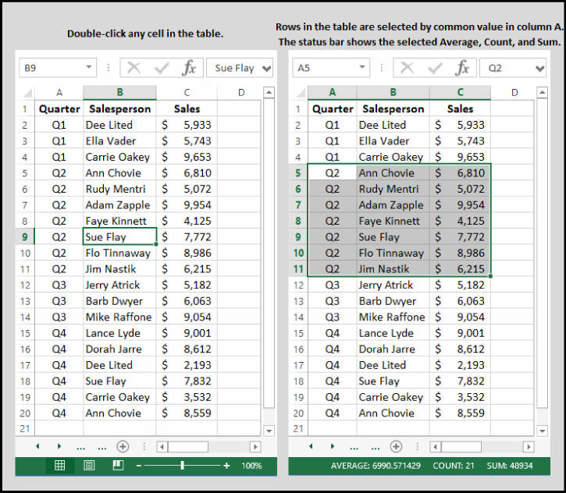
Figure 15.5

NOTE Although this example shows the Select method, you can change the code to a different method, such as to copy or format the range.

One of the conveniences of selecting the relevant range, as shown in Figure 15.5, is to quickly view the selection's calculated information on the status bar. This is a worksheet-level event procedure, so the following code goes into the module of your worksheet:

Private Sub Worksheet_BeforeDoubleClick(ByVal Target As Range, Cancel As Boolean)

'Program only for rows in the list, excluding row 1.

If Target.Row = 1 Then Exit Sub

If Intersect(Target, Range("A1").CurrentRegion) Is Nothing Then Exit Sub

Cancel = True

'Declare variables

Dim myVal As String, LastColumn As Long

Dim Add1 As Long, Add2 As Long

Dim xRow As Long, LastRow As Long

'Define variables

myVal = Cells(Target.Row, 1).Value

LastRow = Cells(Rows.Count, 1).End(xlUp).Row

LastColumn = _

Cells.Find(What:="*", After:=Range("A1"), SearchOrder:=xlByColumns, _

SearchDirection:=xlPrevious).Column

Add1 = Columns(1).Find(What:=myVal, LookIn:=xlValues, LookAt:=xlWhole).Row

xRow = Add1

'Identify the range of rows having the same values in column A.

Do

If Cells(xRow + 1, 1).Value <> myVal Then

Add2 = xRow + 1

Exit Do

Else

xRow = xRow + 1

End If

Loop Until xRow = LastRow

Add2 = xRow

'Select (or copy or format) records having the same values in column A.

Range(Cells(Add1, 1), Cells(Add2, LastColumn)).Select

End Sub

Inserting an Empty Row at Each Change in Items

A common request is how to insert an empty row at each change of data in a column. In Figure 15.6, a table is preferred to be sorted by the Client Name column with an empty row at each change in Client Name. The macro named Sort_Separate_ClientName does that, with comments along the way to explain the process:

Sub Sort_Separate_ClientName()

'Turn off ScreenUpdating.

Application.ScreenUpdating = False

'Sort the table by ClientName in ascending order.

Range("A3").CurrentRegion.Sort _

Key1:=Range("A4"), Order1:=xlAscending, Header:=xlYes

'Declare a Long type variable for the last row in column A.

Dim LastRow As Long

'Determine the last row of data.

LastRow = Cells(Rows.Count, 1).End(xlUp).Row

'Declare a Long type variable for evaluating each row.

Dim xRow As Long

'Loop through each ClientName item in column A of the table.

'When the item being evaluated is not the same as the item

'in the row above it, that means the client name is different.

'Insert an empty row at that change.

'Notice, work from the bottom row upwards because you are

'inserting rows.

For xRow = LastRow To 5 Step -1

If Cells(xRow, 1).Value <> Cells(xRow - 1, 1).Value Then _

Rows(xRow).Resize(1).Insert

Next xRow

'Turn ScreenUpdating on again.

Application.ScreenUpdating = True

End Sub

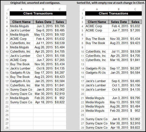
Figure 15.6

Try It

For this lesson, a table of data includes names of stores in column A that are repeated elsewhere in the column. A macro is requested to copy the individual rows of data for each unique store name, and paste those rows into their own workbook.

The workbooks are named by the name of the store, appended with the date and time the macro was run. The workbooks are saved in the same folder path as the workbook holding the original data.

Lesson Requirements

To get the sample workbook, you can download Lesson 15 from the book's website at www.wrox.com/go/excelvba24hour.

Hints

The following hints might help you as you complete this Try It:

· Your list of data need not be too lengthy; a couple dozen rows of data would suffice.

· In the downloadable workbook for this lesson, column A contains a list of store names, which is why you see the references to “Store” in the Step-by-Step code.

· Repeat each item at least once (as mentioned in Step 1), but feel free to repeat each item as many times in column A as you want.

· For convenience, the destination path where the new workbooks will be saved is the same as the path of the workbook holding the original data.

· When you use a helper column or row, be sure to leave at least one empty column or row between it and the data table you are working with. Without the empty column or row, VBA might assume your helper data is a part of the original table.

· When your macros involve creating or working in other workbooks while you refer to a worksheet in your workbook holding the macro, be sure to qualify your worksheet's parent name with the ThisWorkbookobject.

· When your macros create potentially dozens or hundreds of new workbooks, close the workbooks after you name them as shown in Step 24. It's rare for a user to want that many workbooks open at the same time after the macro has completed.

Step-by-Step

1. Start by opening a new workbook and copy or enter a table of data that includes a few columns. Put column labels in row 1, and repeat each of the entries in column A at least once.

2. Save your workbook as a macro-enabled type with the extension .xlsm.

3. Press Alt+F11 to go to the Visual Basic Editor.

4. From the VBE menu bar, click InsertModule.

5. In the module you just created, type Sub UniqueStoresToWorkbooks and press Enter. VBA automatically places a pair of empty parentheses at the end of the Sub line, followed by an empty line, and the End Subline below that. Your macro should look like this so far:

6. Sub UniqueStoresToWorkbooks()

End Sub

6. Turn off ScreenUpdating to speed up the macro when you run it, and to keep your screen from flickering, which happens during macros that manipulate row, column, and workbook objects as this macro does:

Application.ScreenUpdating = False

7. Declare variables:

8. 'Identify and count each row of a unique list of items in column A.

9. Dim UniqueRow As Long, lngUniqueCount As Long

10. 'String variables for each unique item name and its workbook name.

11. Dim strUniqueStore As String, strUniqueStoreWBname As String

12. 'Number of the data table's last row; next available column one column removed

13. 'from the rightmost column of the data table; range occupied by the data table.

14. Dim LastRow As Long, NextColumn As Long, FilterRange As Range

15. 'Path to receive the new workbooks; name of sheet where the data table resides.

Dim strDestinationFolderPath As String, asn As String

8. Define the destination path that will receive the new workbooks, which is the same path of the active workbook holding this macro:

strDestinationFolderPath = ThisWorkbook.Path & "\"

9. Define the sheet name holding the original list:

asn = ActiveSheet.Name

10.Identify the last row in the list, using column A:

LastRow = Cells(Rows.Count, 1).End(xlUp).Row

11.Identify the column that is two columns removed from the right-most column in the list. This column will hold the unique store names, with one empty column separating it from the list:

12. NextColumn = Cells.Find(What:="*", After:=Range("A1"), _

SearchOrder:=xlByColumns, SearchDirection:=xlPrevious).Column + 2

12.Define the range (which is column A of the list) that will be filtered for each unique store name:

13. Set FilterRange = _

ThisWorkbook.Worksheets(asn).Range("A1:A" & LastRow)

13.List all unique store names using AdvancedFilter:

14. FilterRange.AdvancedFilter _

Action:=xlFilterCopy, CopyToRange:=Cells(1, NextColumn), Unique:=True

14.Count the unique store names, not including the header cell. This is a service to the users to let them know in a message box at the end of the macro how many unique items were found, hence how many new workbooks were created:

lngUniqueCount = WorksheetFunction.CountA(Columns(NextColumn)) - 1

15.Open a For…Next loop to loop through all unique store names to be filtered for exposing their respective data:

For UniqueRow = 2 To Cells(Rows.Count, NextColumn).End(xlUp).Row

16.Create the workbook to hold the next unique store name. The 1 in this syntax refers to a standard Excel worksheet:

Workbooks.Add 1

17.Assign the name of the next unique store to the strUniqueStore variable. Turn off AutoFilter first to expose all rows on the worksheet:

18. With ThisWorkbook.Worksheets(asn)

19. .AutoFilterMode = False

20. strUniqueStore = .Cells(UniqueRow, NextColumn).Value

End With

18.Define the full workbook name of the next unique store name, including the extension. The workbook name's date and time suffix helps to reference the creation date at a glance when the workbooks are viewed in Windows File Explorer, and to avoid overriding existing workbook names:

19. strUniqueStoreWBname = strUniqueStore & "_" & _

Format(VBA.Now, "YYYYMMDD_HHMMSS") & ".xlsx"

19.AutoFilter the list for the next unique store name:

FilterRange.AutoFilter Field:=1, Criteria1:=strUniqueStore

20.Copy the visible (filtered) rows for this unique store name, and paste them to the workbook you created for it in Step 16:

FilterRange.SpecialCells(xlCellTypeVisible).EntireRow.Copy Range("A1")

21.Keep in mind that the active workbook at this moment is the new workbook you created for it. The unique list of store names is still visible and not wanted, so clear that column:

Columns(NextColumn).Clear

22.Autofit the columns in this new workbook for readability as a service to the user:

Cells.Columns.AutoFit

23.Save the new workbook:

24. ActiveWorkbook.SaveAs _

25. Filename:=strDestinationFolderPath & _

strUniqueStoreWBname, FileFormat:=51

NOTE In Step 18, the workbooks are saved with the .xlsx extension, which is why the statement FileFormat:=51 is required when naming the files. If you save a workbook with the .xlsmextension, the statement FileFormat:=52 would be required.

24.Close the new workbook:

ActiveWorkbook.Close

25.Continue the loop for all the unique store names:

Next UniqueRow

26.Reactivate this workbook and the worksheet holding the original data table:

27. ThisWorkbook.Activate

Worksheets(asn).Activate

27.Turn off AutoFilter:

ActiveSheet.AutoFilterMode = False

28.Clear the unique list that you created in Step 13:

Columns(NextColumn).Clear

29.Release the FilterRange object variable from system memory:

Set FilterRange = Nothing

30.Turn ScreenUpdating back on:

Application.ScreenUpdating = True

31.With a message box, confirm for the user that the task is completed:

32. MsgBox _

33. "There were " & lngUniqueCount & " different Stores." & vbCrLf & _

34. "Their respective data has been consolidated into" & vbCrLf & _

35. "individual workbooks, all saved in the path" & vbCrLf & _

36. strDestinationFolderPath & ".", vbInformation, "Done!"

End Sub

32.With your macro completed, press Alt+Q to return to the worksheet. To test the macro, press Alt+F8 to show the Macro dialog box. Select the macro named UniqueStoresToWorkbooks and click Run. Here is what the macro looks like in its entirety:

33. Sub UniqueStoresToWorkbooks()

34. 'Turn off screen updating.

35. Application.ScreenUpdating = False

36. 'Declare and define variables.

37. 'Identify and count each row of a unique list of items in column A.

38. Dim UniqueRow As Long, lngUniqueCount As Long

39. 'String variables for each unique item name and its workbook name.

40. Dim strUniqueStore As String, strUniqueStoreWBname As String

41. 'Number of the data table's last row; next available column one column removed

42. 'from the rightmost column of the data table; range occupied by the data table.

43. Dim LastRow As Long, NextColumn As Long, FilterRange As Range

44. 'Path to receive the new workbooks; name of sheet where the data table resides.

45. Dim strDestinationFolderPath As String, asn As String

46. 'Define variables.

47. 'The destination path that will receive these new workbooks

48. 'is the same path as the active workbook.

49. strDestinationFolderPath = ThisWorkbook.Path & "\"

50. 'Start from the sheet name holding the original list.

51. asn = ActiveSheet.Name

52. 'Identify the last cell row of the data table.

53. LastRow = Cells(Rows.Count, 1).End(xlUp).Row

54. 'Identify the column that is 2 columns removed from

55. 'the right-most column in the list.

56. NextColumn = Cells.Find(What:="*", After:=Range("A1"), _

57. SearchOrder:=xlByColumns, _

58. SearchDirection:=xlPrevious).Column + 2

59. 'The range (which is column A of the list) that will be

60. 'filtered for each unique store name.

61. Set FilterRange = _

62. ThisWorkbook.Worksheets(asn).Range("A1:A" & LastRow)

63. 'List all unique Store Names using AdvancedFilter.

64. FilterRange.AdvancedFilter Action:=xlFilterCopy, _

65. CopyToRange:=Cells(1, NextColumn), Unique:=True

66. 'Count the unique Stores, not including the header cell.

67. 'This is a service to the user to let them know in a message box

68. 'at the end of the macro how many unique items were found,

69. 'meaning how many new workbooks were created.

70. lngUniqueCount = WorksheetFunction.CountA(Columns(NextColumn)) - 1

71. 'Open a For…Next loop, to loop through all

72. 'unique store names, filter for them, and paste their data to a

73. 'new workbook, saved with creation date and time.

74. For UniqueRow = 2 To Cells(Rows.Count, NextColumn).End(xlUp).Row

75. 'Create the workbook to hold the next unique store name.

76. Workbooks.Add 1

77. 'Assign the name of the next unique store to

78. 'the strUniqueStore variable.

79. 'AutoFilter is turned off first to expose all rows on the sheet.

80. With ThisWorkbook.Worksheets(asn)

81. .AutoFilterMode = False

82. strUniqueStore = .Cells(UniqueRow, NextColumn).Value

83. End With

84. 'Define the full workbook name of the next

85. 'unique store name, including extension.

86. 'The workbook name's date and time suffix helps to

87. 'reference the creation date at a glance when the

88. 'workbooks are viewed in Windows File Explorer,

89. 'and to avoid overriding existing workbook names.

90. strUniqueStoreWBname = strUniqueStore & "_" & _

91. Format(VBA.Now, "YYYYMMDD_HHMMSS") & ".xlsx"

92. 'Filter the list for that next unique store name.

93. FilterRange.AutoFilter Field:=1, Criteria1:=strUniqueStore

94. 'Copy the visible (filtered) rows for this unique

95. 'store name, and paste them to their new workbook.

96. FilterRange.SpecialCells(xlCellTypeVisible).EntireRow.Copy Range("A1")

97. 'Keep in mind that the active workbook at this moment

98. 'is the new workbook you created for it. The unique list of

99. 'store names is still visible and not needed, so clear that column.

100. Columns(NextColumn).Clear

101. 'Autofit the columns in this new workbook for readability.

102. Cells.Columns.AutoFit

103. 'Save and close the new workbook.

104. ActiveWorkbook.SaveAs _

105. Filename:=strDestinationFolderPath & _

106. strUniqueStoreWBname, FileFormat:=51

107. 'Close the new workbook.

108. ActiveWorkbook.Close

109. 'Continue the loop through all the unique store names.

110. Next UniqueRow

111. 'Re-activate this workbook and the source worksheet.

112. ThisWorkbook.Activate

113. Worksheets(asn).Activate

114. 'Turn off autofilter.

115. ActiveSheet.AutoFilterMode = False

116. 'Clear the unique list.

117. Columns(NextColumn).Clear

118. 'Release the object variable from system memory.

119. Set FilterRange = Nothing

120. 'Turn screen updating back on.

121. Application.ScreenUpdating = True

122. 'Confirm for the user that the parsing is completed.

123. MsgBox _

124. "There were " & lngUniqueCount & " different Stores." _

125. & vbCrLf & _

126. "Their respective data has been consolidated into" & _

127. vbCrLf & _

128. "individual workbooks, all saved in the path" & vbCrLf & _

129. strDestinationFolderPath & ".", vbInformation, "Done!"

End Sub

REFERENCE Please select the video for Lesson 15 at www.wrox.com/go/excelvba24hour. You will also be able to download the code and resources for this lesson from the website.

All materials on the site are licensed Creative Commons Attribution-Sharealike 3.0 Unported CC BY-SA 3.0 & GNU Free Documentation License (GFDL)

If you are the copyright holder of any material contained on our site and intend to remove it, please contact our site administrator for approval.

© 2016-2026 All site design rights belong to S.Y.A.