Excel VBA 24-Hour Trainer (2015)

Part III
Beyond the Macro Recorder: Writing Your Own Code

Lesson 16
Using Embedded Controls

You've seen many ways to run macros, including using keyboard shortcuts, the Macro dialog box, and the Visual Basic Editor. This lesson shows you how to execute VBA code by clicking a button or other object that you can place onto your worksheet to make your macros easier to run.

Working with Form Controls and ActiveX Controls

A control is an object such as a Button, Label, TextBox, OptionButton, or CheckBox that you can place onto a UserForm (covered in Lessons 21, 22, and 23) or embed onto a worksheet. VBA supports these and more controls, which provide an intuitive way for you to run your macros quickly and with minimal effort.

Excel supports two generations of controls. Form controls are the original controls that came with Excel, starting with version 5. Form controls are still fully supported in all later versions of Excel, including Excel 2013. Form controls are more stable, simpler to use, and more integrated with Excel. For example, you can place a Form control onto a chart sheet, but you cannot do that with an ActiveX control.

Generally, ActiveX controls from the Control Toolbox are more flexible with their extensive properties and events. You can customize their appearance, behavior, fonts, and other characteristics. You can also control how different events are responded to when an ActiveX control is associated with those events.

Form controls have macros that are assigned to them. ActiveX controls run procedures that are based on whatever event(s) they have been programmed to monitor. ActiveX controls don't look all that scintillating, but Form controls have an even more elementary appearance that will never win them first prize in a beauty contest. However, both kinds of controls serve their purposes well as Microsoft intended, and they are here to stay with Excel for the foreseeable future.

CHOOSING BETWEEN FORM CONTROLS AND ACTIVEX CONTROLS

The primary differences between the two kinds of controls are in formatting and events. You use Form controls when you need simple interaction with VBA, such as running a macro by clicking a button. They are also a good choice when you don't need VBA at all, but you want an option button or check box on your sheet that will be linked to a cell. If you need to color your control, or format its font type, or trigger a procedure based on mouse movement or keyboard activity, ActiveX controls are the better choice.

Be aware that ActiveX controls have a well-deserved reputation for being buggy and not behaving as reliably as do Form controls. Form controls will give you minimal problems, if any, but they are limited in what they can do. As you experiment and work with each type, you'll decide which kind of control works best for your purposes.

The Forms Toolbar

The easiest way to access Form controls is through the Forms toolbar. How you get to the Forms toolbar depends on your version of Excel. For versions prior to Excel 2007, from the worksheet menu, click ViewToolbarsForms, as shown in Figure 16.1.

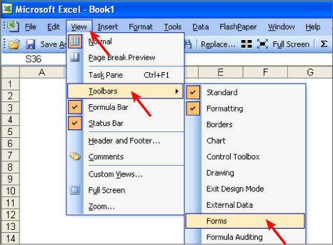
Figure 16.1

The Forms toolbar is like any other toolbar that you can dock at the top or sides of the window, or have floating on the window above the worksheet. Figure 16.2 shows the Forms toolbar and its control icons.

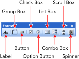
Figure 16.2

If you are using Excel version 2007, 2010, or 2013, you get to the Forms and ActiveX controls by clicking the Insert icon on the Developer tab of the Ribbon, as shown in Figure 16.3.

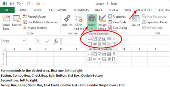
Figure 16.3

NOTE The Developer tab is a very useful item to place on your Ribbon. See the “Accessing the VBA Environment” section in Lesson 2 for the steps to display the Developer tab.

Buttons

The most commonly used Form control is the Button. When you use a Button, you have a macro in mind that you have either already written or will write, which will be attached to the Button. The following steps are a common sequence of actions when using a Form Button:

1. Create the macro that will be attached to the Button. Suppose you are negotiating rents, and you need to frequently clear the range C4:F4 on a company budget sheet. The macro you'd write is

2. Sub ClearData()

3. Range("C4:F4").Clear

End Sub

2. To make it easy to run that macro, you can assign it to a Form Button. On the Forms toolbar, click the Button icon. Press down your mouse's left button, then draw the Button into cell B4. As soon as you do, the Assign Macro dialog box appears, as shown in Figure 16.4. Select the macro to be assigned to the Button, and click OK.

3. With your new Button selected, click it and delete the entire default caption. Type the caption Clear Cells, as shown in Figure 16.5.

4. Select any worksheet cell to deselect the Button. Go ahead and click the Button to verify that it clears the cells in range C4:F4 as expected.

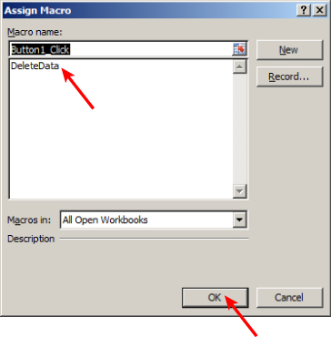
Figure 16.4

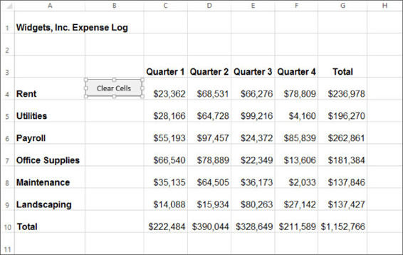
Figure 16.5

Using Application.Caller with Form Controls

One of the cool things about Form controls is that you can apply a single macro to all of them and gain information about which control was clicked. When you know which Button was clicked, you can take a specific action relating to that Button.

Expanding on the previous example, suppose you want to place a Button on each row of data, so that when you click a Button, the cells are cleared in columns C:F of the row where the Button resides. It's obvious that the original macro applies only to the first Button in the Rent row, so here are the steps to have one macro serve many controls:

1. Modify the ClearData macro as follows. For the Button that was clicked, the cell holding that Button's top-left corner is identified. The macro can now be a customization tool for each individual Button to which it is attached:

2. Sub ClearData()

3. Dim myRow As Long

4. myRow = _

5. ActiveSheet.Buttons(Application.Caller).TopLeftCell.Row

6. Range(Cells(myRow, 3), Cells(myRow, 6)).Clear

End Sub

2. Recall that the original macro name is still attached to that Button. Return to your worksheet and right-click the Button. Select Copy because you are copying the Button and the macro to which it is attached.

3. Select cell B5 and press Ctrl+V. Repeat that step for cells B6, B7, B8, and B9. Your worksheet will resemble Figure 16.6.

4. Test the macro by clicking the Button on the Office Supplies row. When you click that Button, the macro clears the cells in row 7, columns C:F, as shown in Figure 16.7.

NOTE Attaching a macro to an embedded object is not limited to Form controls. You can attach a macro to pretty much any Drawing shape or picture that you want to embed onto your worksheet.

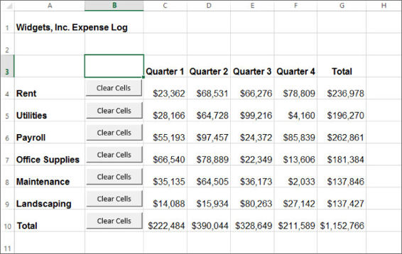
Figure 16.6

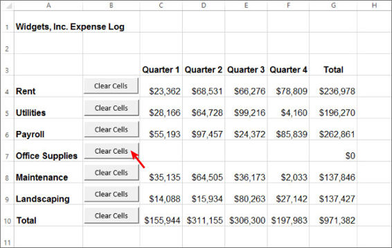
Figure 16.7

The Control Toolbox

Similar to the Forms toolbar, the Control Toolbox can be accessed in versions prior to Excel 2007 from the worksheet menu bar. Click ViewToolbarsControl Toolbox, as shown in Figure 16.8.

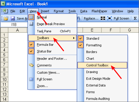
Figure 16.8

The Control Toolbox itself is shown in Figure 16.9. If you are using version 2007, 2010, or 2013, you can find the Forms and ActiveX controls by clicking the Insert icon on the Developer tab of the Ribbon, shown in Figure 16.9.

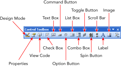
Figure 16.9

More than 100 additional ActiveX controls beyond what you see on the Control Toolbox are available. You might notice an icon named More Controls at the far right of the Control Toolbox toolbar, and in the lower-right corner of the Insert icon's drop-down display in Excel 2007, 2010, and 2013. When expanded, that icon (see Figure 16.10), reveals the additional ActiveX controls available for you to embed, as indicated in Figure 16.11.

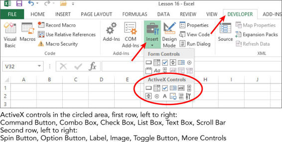
Figure 16.10

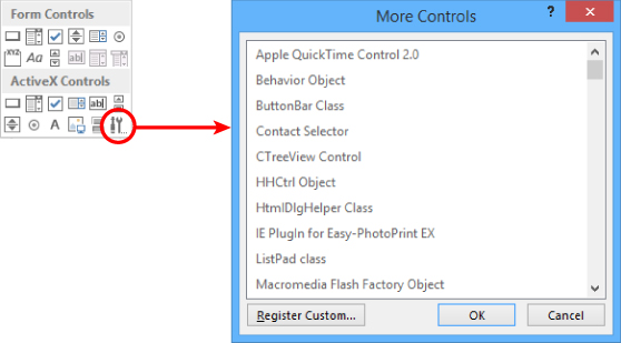
Figure 16.11

NOTE The odds are you'll never need most of those controls, but it gives you a sense of the expansive functionality that is available to you with ActiveX objects.

CommandButtons

The ActiveX CommandButton is the counterpart to the Form control button. As with virtually every ActiveX object, the CommandButton has numerous properties through which you can customize its appearance. Unlike Form controls, an ActiveX object such as a CommandButton responds to event code. There is no such thing as a macro being attached to a CommandButton.

From the Control Toolbox, draw a CommandButton onto your worksheet. Excel defaults to Design Mode, allowing you to work with the ActiveX object you just created. Right-click the CommandButton and select Properties, as shown in Figure 16.12. You can see the Design Mode icon is active.

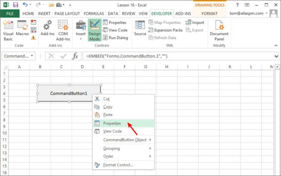
Figure 16.12

You will see the Properties window for the CommandButton, where you can modify a number of properties. Change the Caption property of the CommandButton to CheckBox Checker, as shown in Figure 16.13.

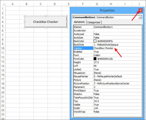
Figure 16.13

Draw a Label control and four CheckBoxes from the Control Toolbox below the CommandButton. In Figure 16.14, I changed the Label's caption to Check Your Favorite Activities. I changed each CheckBox's caption to a different leisure activity.

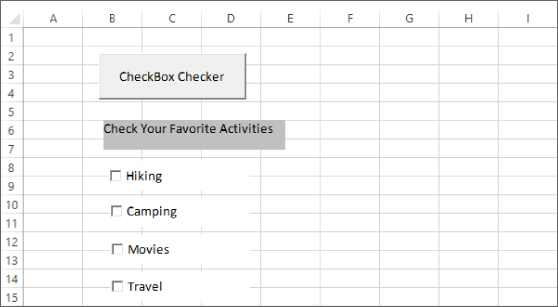
Figure 16.14

Either double-click the CommandButton, or right-click it and select View Code. Either way, you go to the worksheet module and the default Click event is started for you with the following entry:

Private Sub CommandButton1_Click()

End Sub

NOTE VBA code for embedded ActiveX objects is almost always in the module of the worksheet upon which the objects are embedded.

For this demonstration, when the CommandButton is clicked, it evaluates every embedded object on the worksheet. When the code comes across an ActiveX CheckBox, it determines whether the CheckBox is checked. At the end of the procedure, a message box appears, confirming how many (if any) CheckBoxes were checked, and their captions. The entire code looks as follows:

Private Sub CommandButton1_Click()

'Evaluate which checkboxes are checked.

'Declare an Integer type variable to help

'count through the CheckBoxes,'and an Object

'type variable to identify the kind of ActiveX control

'(checkboxes in this example) that are selected.

Dim intCounter As Integer, xObj As OLEObject

'Declare a String variable to list the captions

'of selected checkboxes.

Dim strObj As String

'Start the Integer and String variables.

intCounter = 0

strObj = ""

For Each xObj In ActiveSheet.OLEObjects

If TypeName(xObj.Object) = "CheckBox" Then

If xObj.Object.Value = True Then

intCounter = intCounter + 1

strObj = strObj & xObj.Object.Caption & Chr(10)

End If

End If

Next xObj

'Advise the user of your findings.

If intCounter = 0 Then

MsgBox "No CheckBoxes were selected.", , "Try to get out more often!"

Else

MsgBox "You selected " & intCounter & " CheckBox(es):" & vbCrLf & vbCrLf & _

strobj, , "Here is what you checked:"

End If

End Sub

Leave the VBE and return to the worksheet by pressing Alt+Q. Click the Design Mode button to exit Design Mode. Figure 16.15 shows where the Design Mode icon is on the Developer tab.

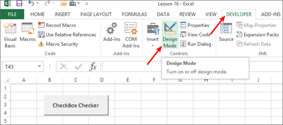
Figure 16.15

With Design Mode now off, you can test the Click event code for the ActiveX CommandButton. Figure 16.16 shows an example of the confirming message box when you click the CommandButton.

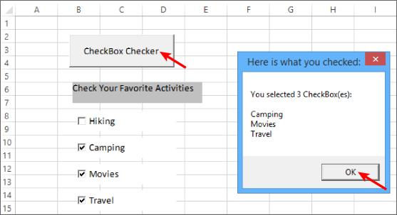
Figure 16.16

Try It

For this lesson, you place a Form Button on a worksheet that contains a hypothetical table of monthly income activity for a department store's clothing items. You attach a macro to the Button that, when clicked, toggles columns or rows as being hidden or visible, depending on how you want to see the data. Upon each click of the Button, the cycle of views will be to see the entire table's detail, see totals only by clothing item, or see totals only by month. This lesson also includes tips on fast data entry by using the fill handle and shortcut keys.

Lesson Requirements

To get the sample workbook you can download Lesson 16 from the book's website at www.wrox.com/go/excelvba24hour.

Step-by-Step

1. Open Excel and open a new workbook.

2. On your active worksheet, list the months of the year in range A6:A17. You can do this quickly by entering January in cell A6, then selecting A6, and pointing your mouse over the fill handle, which is the small black square in the lower-right corner of the selected cell. You know your mouse is hovering over the fill handle when the cursor changes to a crosshairs, as indicated in Figure 16.17. Press your left mouse button onto the fill handle, and drag your mouse down to cell A17 as indicated in Figure 16.18. Release the mouse button, and the 12 months of the year fill into range A6:A17 as shown in Figure 16.19.

3. Enter some clothing items into range B5:F5.

4. Enter sample numbers in range B6:F17. There is nothing special about the numbers; they are just for demonstration purposes. To enter the numbers quickly, as shown in Figure 16.20, do the following:

· Select range B6:F17.

· Type the formula =INT(RAND()*1000).

· Press Ctrl+Enter.

· Press Ctrl+C to copy the range.

· Right-click somewhere in the range B6:F17, and select Paste SpecialValuesOK.

· Press the Esc key to exit Copy mode.

5. In cell G5 enter Total and in cell A18 enter Total.

6. Select the column A header, which selects all of column A. Right-click any cell in column A, select Column Width, enter 20, and click OK.

7. Quickly enter Sum functions for all rows and columns. Select range B6:G18, as shown in Figure 16.21, and either double-click the Sum function icon or press Alt+=.

8. With range B6:G18 currently selected, right-click anywhere in the selection, select Format Cells, and click the Number tab in the Format Cells dialog box. In the category pane select Currency, set Decimal Places to 0, and click OK as indicated in Figure 16.22. Your final result should resemble Figure 16.23, with different numbers because they were produced with the RAND function, but all good enough for this lesson.

9. The task at hand is to create a macro that will be attached to a Form Button. Each time you click the Button, the macro toggles to the next of three different views of the table: seeing the entire table's detail, seeing totals only by clothing item, or seeing totals only by month. To get started, press Alt+F11 to go to the Visual Basic Editor.

10.From the VBE menu bar, click InsertModule.

11.In your new module, type Sub ToggleViews and press Enter. VBA produces the following two lines of code, with an empty row between them:

12. Sub ToggleViews()

End Sub

12.Because the macro hides and unhides rows and columns, turn off ScreenUpdating to keep the screen from flickering:

Application.ScreenUpdating = False

13.Open a With structure that uses Application.Caller to identify the Form Button that was clicked:

With ActiveSheet.Buttons(Application.Caller)

14.Toggle between views based on the Button's captions to determine which view is next in the cycle:

15. If .Caption = "SHOW ALL" Then

16. With Range("A5:G18")

17. .EntireColumn.Hidden = False

18. .EntireRow.Hidden = False

19. End With

20. .Caption = "MONTH TOTALS"

21. ElseIf .Caption = "MONTH TOTALS" Then

22. Range("B:F").EntireColumn.Hidden = True

23. .Caption = "ITEM TOTALS"

24. ElseIf .Caption = "ITEM TOTALS" Then

25. Range("B:F").EntireColumn.Hidden = False

26. Rows("6:17").Hidden = True

27. .Caption = "SHOW ALL"

End If 'for evaluating the button caption.

15.Close the With structure for Application.Caller:

End With

16.Turn ScreenUpdating on again:

Application.ScreenUpdating = True

17.Your entire macro looks like this:

18. Sub ToggleViews()

19. 'Turn off ScreenUpdating.

20. Application.ScreenUpdating = False

21. 'Open a With structure that uses Application.Caller

22. 'to identify the Form Button that was clicked.

23. With ActiveSheet.Buttons(Application.Caller)

24. 'Toggle between views based on the Button's captions

25. 'to determine which view is next in the cycle.

26. If .Caption = "SHOW ALL" Then

27. With Range("A5:G18")

28. .EntireColumn.Hidden = False

29. .EntireRow.Hidden = False

30. End With

31. .Caption = "MONTH TOTALS"

32. ElseIf .Caption = "MONTH TOTALS" Then

33. Range("B:F").EntireColumn.Hidden = True

34. .Caption = "ITEM TOTALS"

35. ElseIf .Caption = "ITEM TOTALS" Then

36. Range("B:F").EntireColumn.Hidden = False

37. Rows("6:17").Hidden = True

38. .Caption = "SHOW ALL"

39. End If 'for evaluating the Button caption.

40. 'Close the With structure for Application.Caller.

41. End With

42. 'Turn ScreenUpdating on again.

43. Application.ScreenUpdating = True

End Sub

18.Press Alt+Q to return to the worksheet.

19.Draw a Form Button on your worksheet at the top of column A. When you release the mouse button you see the Assign Macro dialog box. Select the macro named ToggleViews and click OK, as shown in Figure 16.24.

20.Make sure the Button is totally within column A, as indicated in Figure 16.25. Right-click the Button and select Edit Text.

21.Change the Button's caption to SHOW ALL, as shown in Figure 16.26.

22.Select any cell to deselect the Button. Click the Button once and nothing changes on the sheet because all the columns and rows are already visible. You see that the Button's caption changed to MONTH TOTALS. If you click the Button again, you see the month names listed in column A, and their totals listed in column G. The Button's caption reads ITEM TOTALS. Click the Button again to see the clothing items named in row 5, and their totals listed in row 18. The Button's caption reads SHOW ALL, and if you click the Button again, all rows and columns are shown.

23.You can continue cycling through the table's views by clicking the Form Button for each view that you coded into the ToggleViews macro.

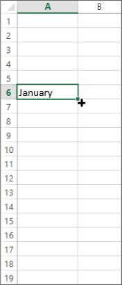
Figure 16.17

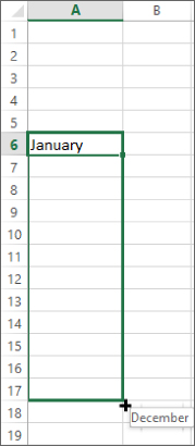
Figure 16.18

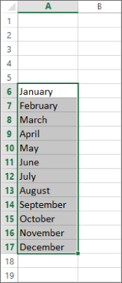
Figure 16.19

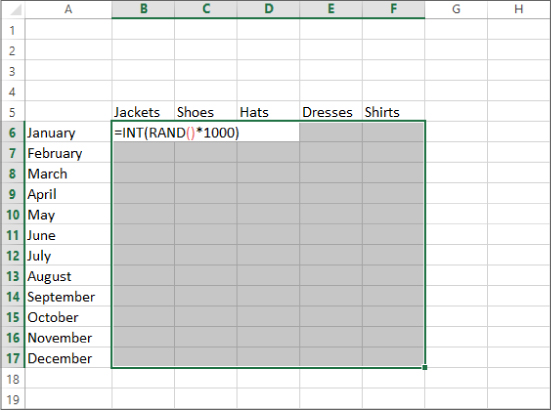
Figure 16.20

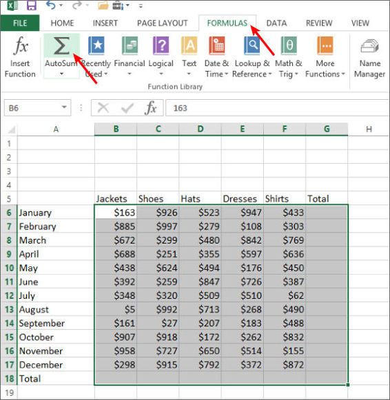
Figure 16.21

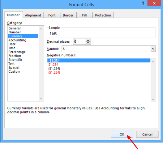
Figure 16.22

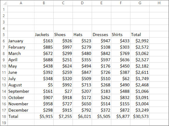
Figure 16.23

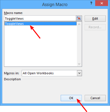
Figure 16.24

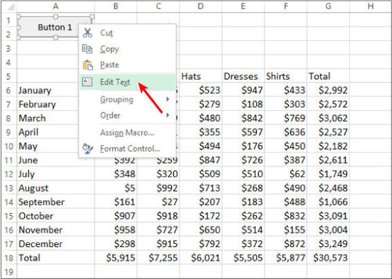
Figure 16.25

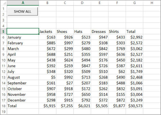
Figure 16.26

REFERENCE Please select the video for Lesson 16 at www.wrox.com/go/excelvba24hour. You will also be to download the code and resources for this lesson from the website.