Excel VBA 24-Hour Trainer (2015)

Part III
Beyond the Macro Recorder: Writing Your Own Code

Lesson 17
Programming Charts

When I started to program Excel in the early 1990s, I remember being impressed with the charting tools that came with Excel. They were very good back then, and today's chart features in Excel are downright awesome, rivaling—and usually surpassing—the charting packages of any software application.

Because you are reading this book, chances are pretty good that you've manually created your share of charts in Excel using the Chart Wizard or by selecting a chart type from the dozens of choices on the Ribbon. You might also have played with the Macro Recorder to do some automation of chart creation. This lesson takes you past the Macro Recorder's capabilities to show how to create and manipulate embedded charts and chart sheets.

The topic of charting is one that can, and does, fill entire books. The myriad chart types and features that Excel makes available to you goes well beyond the scope of this lesson. What this lesson does is show you the syntaxes for several methods that work for embedded charts and chart sheets, with a few different features and chart types represented in the programming code. From the VBA examples in this lesson, you can expand your chart programming skills by substituting the chart types and features shown for others that may be more suited to the kinds of charts you want to develop.

NOTE In the examples, you might notice that the charts being created are declared as a Chart type object variable, which makes it easier to refer to the charts when you want to manipulate them in code. In any case, Excel has two separate object models for charts. For a chart on its own chart sheet, it is a Chart object. For a chart embedded on a worksheet, it is a ChartObject object. Chart sheets are members of the workbook's Charts collection, and each ChartObject on a worksheet is a member of the worksheet's ChartObjects collection.

Adding a Chart to a Chart Sheet

As you know, a chart sheet is a special kind of sheet in your workbook that contains only a chart. If the chart is destined to be large and complicated, users often prefer such a chart be on its own sheet so they can view its detail more easily.

Figure 17.1 shows a table of sales by month for a company that is the source data for this chart example. The table is on Sheet1, and although you can correctly refer to the source range in your code as A1:B13, I prefer using the CurrentRegion property to reduce the chances of entering the wrong range reference in my code.

The following macro creates a column chart for a new chart sheet based on the data in Figure 17.1. If the Location property of your Chart object has not been specified, as it has not been in this macro, your chart is created in its own chart sheet. The result of this new chart sheet is shown in Figure 17.2.

Sub CreateChartSheet()

'Declare your chart type object variable.

Dim myChart1 As Chart

'Set your variable to add a chart.

Set myChart1 = Charts.Add

'Define the new chart's source data.

myChart1.SetSourceData _

Source:=Worksheets("Sheet1").Range("A1").CurrentRegion, _

PlotBy:=xlColumns

'Define the type of chart.

myChart1.ChartType = xlColumnClustered

'Delete the legend because it is redundant with the chart title.

ActiveChart.Legend.Delete

End Sub

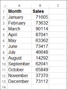
Figure 17.1

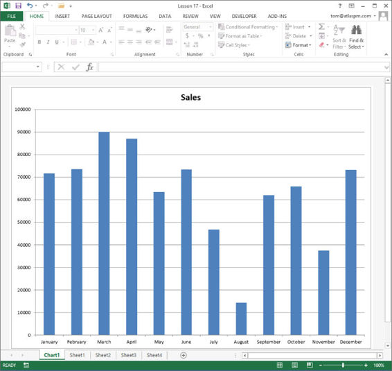
Figure 17.2

NOTE To change your default type of chart, right-click any chart in your workbook and select Change Chart Type. In the Change Chart Type dialog box, select a chart type, click the Set as Default Chart button, and click OK. In version 2013, right-click a chart type and select Set as Default Chart.

Simply executing the code line Charts.Add in the Immediate window creates a new chart sheet. If the active cell were within a table of data, your default type chart would occupy the new chart sheet, representing the table, or more precisely, the data within the CurrentRegion property of the selected cell. If you did not have any data selected at the time, a new chart sheet would still be created, with a blank Chart object looking like an empty canvas waiting to be supplied with source data.

DID YOU KNOW…

If the active cell is within a table of data, or you have a range of data selected, and you press the F11 key, a new chart sheet is added to hold a chart that represents the selected data. Some people find this to be an annoyance because they have no interest in charts, and may not be aware they touched the F11 key when a chart sheet has appeared out of nowhere.

If you want to negate the effect of pressing the F11 key, you can place the following OnKey procedures into the ThisWorkbook module. Some Excel users who frequently use the F2 key to get into Edit mode sometimes press the F1 Help key by mistake and nullify the F1 key in this fashion as well:

Private Sub Workbook_Open()

Application.OnKey "{F11}", ""

End Sub

Private Sub Workbook_Activate()

Application.OnKey "{F11}", ""

End Sub

Private Sub Workbook_Deactivate()

Application.OnKey "{F11}"

End Sub

Private Sub Workbook_BeforeClose(Cancel As Boolean)

Application.OnKey "{F11}"

End Sub

Adding an Embedded Chart to a Worksheet

When you embed a chart in a worksheet, there is more to consider than when you create a chart for its own chart sheet. When you embed a chart, you need to specify which worksheet you want the chart to be on (handled by the Location property), and where on the worksheet you want the chart to be placed. The following macro is an example of how to place a column chart into range D3:J20 of the active worksheet, close to the source range, as shown in Figure 17.3:

Sub CreateChartSameSheet()

'Declare an Object variable for the chart

'and for the embedded ChartObject.

Dim myChart1 As Chart, cht1 As ChartObject

'Declare a Range variable to specify what range

'the chart will occupy, and on what worksheet.

Dim rngChart1 As Range, DestinationSheet As String

'The chart will be placed on the active worksheet.

DestinationSheet = ActiveSheet.Name

'Add a new chart

Set myChart1 = Charts.Add

'Specify the chart's location as the active worksheet.

Set myChart1 = _

myChart1.Location _

(Where:=xlLocationAsObject, Name:=DestinationSheet)

'Define the new chart's source data

myChart1.SetSourceData _

Source:=Range("A1").CurrentRegion, PlotBy:=xlColumns

'Define the type of chart, in this case, a Column chart.

myChart1.ChartType = xlColumnClustered

'Activate the chart to identify its ChartObject.

'The (1) assumes this is the first (index #1) chart object

'on the worksheet.

ActiveSheet.ChartObjects(1).Activate

Set cht1 = ActiveChart.Parent

'Specify the range you want the chart to occupy.

Set rngChart1 = Range("D3:J20")

cht1.Left = rngChart1.Left

cht1.Width = rngChart1.Width

cht1.Top = rngChart1.Top

cht1.Height = rngChart1.Height

'Deselect the chart by selecting a cell.

Range("A1").Select

End Sub

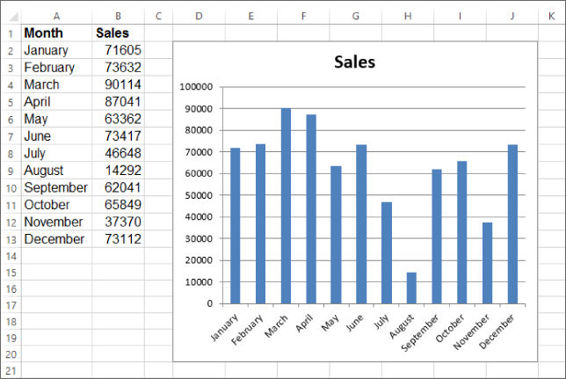
Figure 17.3

WARNING Here's a cool tip: Starting with version 2010, you can select any cell in a table of data, then press Alt+F1 to embed a chart of that data onto your worksheet. From there, you can drag the chart to your preferred location on the worksheet.

NOTE One of the best practice items in VBA programming that I mention throughout the book, and you will see posted in newsgroups ad nauseam, is to avoid selecting or activating objects in your VBA code. Most of the time that is good advice. However, sometimes you need to select objects to refer reliably to them or to manipulate them, and the preceding macro demonstrated two examples. The ChartObject was activated to derive the actual name of the chart. Also, the macro ended with cell A1 being selected. You could select any cell or any object, but a cell—any cell—is the safest object to select after creating a new embedded chart. Any code that is executed after adding a new chart might not execute correctly if the ChartObject is still selected. The most reliable way to deselect a chart at the end of your macro is to select a cell.

Moving a Chart

You can change the location of any chart, which you might be familiar with if you've right-clicked a chart's area and noticed the Move Chart menu item. The following scenarios show how to do this with VBA.

To move a chart from a chart sheet to a worksheet, select the chart sheet programmatically and specify the worksheet where you want the chart to be relocated. It's usually a good idea to tell VBA where on the worksheet you want the chart to go; otherwise, the chart is plopped down on the sheet wherever VBA decides. That is why the code in the With structure specifies that cell C3 be the top-left corner of the relocated chart:

Sub ChartSheetToWorksheet()

'Chart1 is the name of the chart sheet.

Sheets("Chart1").Select

'Move the chart to Sheet1.

ActiveChart.Location Where:=xlLocationAsObject, Name:="Sheet1"

'Cell C3 is the top left corner location of the chart.

With Worksheets("Sheet1")

ActiveChart.Parent.Left = .Range("C3").Left

ActiveChart.Parent.Top = .Range("C3").Top

End With

'Deselect the chart.

Range("A1").Select

End Sub

To move a chart from a worksheet to a chart sheet, you need to determine the name or index number of your chart. If you have only one chart on your worksheet, you know that chart's index property is 1, but specifying the chart by its name is a safe way to go. The code is much simpler because a chart sheet can contain only one chart, so you don't need to specify a location on the chart sheet itself:

Sub EmbeddedChartToChartSheet()

ActiveSheet.ChartObjects("Chart 1").Activate

ActiveChart.Location Where:=xlLocationAsNewSheet, Name:="Chart1"

End Sub

NOTE You can determine the name of any embedded chart quickly by selecting it to see its name in the Name box.

To move an embedded chart from one worksheet to another, it's the same concept of specifying which chart to move, and which worksheet to move it to:

Sub EmbeddedChartToAnotherWorksheet()

'Chart 5 is the name of the chart to move to Sheet2.

ActiveSheet.ChartObjects("Chart 5").Activate

ActiveChart.Location Where:=xlLocationAsObject, Name:="Sheet2"

'Cell B6 is the top left corner location of the chart.

With Worksheets("Sheet2")

ActiveChart.Parent.Left = .Range("B6").Left

ActiveChart.Parent.Top = .Range("B6").Top

End With

'Deselect the chart.

Range("A1").Select

End Sub

You can quickly move all chart sheets to their own workbook. For example, check out the following example that creates a new workbook and relocates the chart sheets before Sheet1 in that new workbook:

Sub ChartSheetsToWorkbook()

'Declare variable for your active workbook name.

Dim myName As String

'Define the name of your workbook.

myName = ActiveWorkbook.Name

'Add a new Excel workbook.

Workbooks.Add 1

'Copy the chart sheets from your source workbook

'to the new workbook.

Workbooks(myName).Charts.Move before:=Sheets(1)

End Sub

Looping Through All Embedded Charts

Suppose you want to do something to every embedded chart in your workbook. For example, if some charts were originally created with different background colors, you might want to standardize the look of all charts to have the same color scheme. The following macro shows how to loop through every chart on every worksheet to format the chart area with a standard color of cyan:

Sub LoopAllEmbeddedCharts()

'Turn off ScreenUpdating.

Application.ScreenUpdating = False

'Declare variables for worksheet and chart objects.

Dim wks As Worksheet, ChObj As ChartObject

'Open loop for every worksheet.

For Each wks In Worksheets

'Determine if the worksheet has at least one chart.

If wks.ChartObjects.Count > 0 Then

'If the worksheet has a chart, activate the worksheet.

wks.Activate

'Loop through each chart object.

For Each ChObj In ActiveSheet.ChartObjects

'Activate the chart.

ChObj.Activate

'Color the chart area cyan.

ActiveChart.ChartArea.Interior.ColorIndex = 8

'Deselect the active chart before proceeding to the

'next chart or the next worksheet.

Range("A1").Select

'Continue and close the loop for every chart on that sheet.

Next ChObj

'Close the If structure if the worksheet had no chart.

End If

'Continue and close the loop for every worksheet.

Next wks

'Turn on ScreenUpdating.

Application.ScreenUpdating = True

End Sub

If you have chart sheets to be looped through, the code must be different to take into account the type of sheet to look for, because a chart sheet is a different type of sheet than a worksheet. This macro accomplishes the same task of coloring the chart area, but for charts on chart sheets:

Sub LoopAllChartSheets()

'Turn off ScreenUpdating.

Application.ScreenUpdating = False

'Declare an object variable for the Sheets collection.

Dim objSheet As Object

'Loop through all sheets, only looking for a chart sheet.

For Each objSheet In ActiveWorkbook.Sheets

If TypeOf objSheet Is Excel.Chart Then

'Activate the chart sheet.

objSheet.Activate

'Color the chart area cyan.

ActiveChart.ChartArea.Interior.ColorIndex = 8

'Close the If structure and move on to the next sheet.

End If

Next objSheet

'Turn on ScreenUpdating.

Application.ScreenUpdating = True

End Sub

Deleting Charts

To delete all charts on a worksheet, you can execute this code line in the Immediate window, or as part of a macro:

If activesheet.ChartObjects.Count > 0 Then ActiveSheet.ChartObjects.Delete

To delete chart sheets, loop through each sheet starting with the last sheet, determine whether the sheet is a chart sheet, and if so, delete it.

NOTE This loop starts from the last sheet and moves backward using the Step -1 statement. It's a wise practice to loop backward when deleting sheets, rows, or columns. Behind the scenes, VBA relies on the counts of objects in collections, and where the objects are located relative to the others. Deleting objects starting at the end and working your way to the beginning keeps VBA's management of those objects in order.

Sub DeleteChartSheets()

'Turn off ScreenUpdating. Also turn off the Alerts feature,

'so when you delete a sheet VBA does not warn you.

With Application

.ScreenUpdating = False

.DisplayAlerts = False

'Declare an Integer variable for the count of all Sheets.

Dim intSheet As Integer

'Loop through all sheets, only looking for a chart sheet.

For intSheet = Sheets.Count To 1 Step -1

If TypeName(Sheets(intSheet)) = "Chart" Then Sheets(intSheet).Delete

Next intSheet

'Turn on ScreenUpdating and DisplayAlerts.

.DisplayAlerts = True

.ScreenUpdating = True

End With

End Sub

Renaming a Chart

As you have surely noticed when creating objects such as charts, pivot tables, or drawing objects, Excel has a refined knack for giving those objects the blandest default names imaginable. Suppose you have three embedded charts on your worksheet. The following macro changes the names of those charts to something more meaningful:

Sub RenameCharts()

With ActiveSheet

.ChartObjects(1).Name = "Monthly Income"

.ChartObjects(2).Name = "Monthly Expense"

.ChartObjects(3).Name = "Net Profit"

End With

End Sub

Try It

In this lesson you create an embedded pie chart, position it near the source data, and give each legend key a unique color. The pie has four slices; each has a unique color and displays its respective data label.

Lesson Requirements

To get the sample database files you can download Lesson 17 from the book's website at www.wrox.com/go/excelvba24hour.

Step-by-Step

1. Insert a new worksheet and construct the simple table, as shown in Figure 17.4.

2. From your worksheet, press Alt+F11 to go to the Visual Basic Editor.

3. From the VBE menu bar, click InsertModule.

4. In your new module, enter the name of this macro, which I am calling TryItPieChart. Type Sub TryItPieChart, press Enter, and VBA produces the following code:

5. Sub TryItPieChart()

End Sub

5. Declare the ChartObject variable:

Dim chtQuarters As ChartObject

6. Set the variable to the chart being added. Position the chart near the source data:

7. Set chtQuarters = _

8. ActiveSheet.ChartObjects.Add _

(Left:=240, Width:=340, Top:=5, Height:=240)

NOTE The data components inside the parentheses tell VBA where to position your new chart on the worksheet.

1. The Left parameter defines the position in points of the left edge of the ChartObject relative to the left edge of the worksheet.

2. The Top parameter defines the position in points of the top of the ChartObject relative to the top of the worksheet.

3. The Width parameter defines the ChartObject's width, in points.

4. The Height parameter defines the ChartObject's height, in points.

5. A point is a small unit of measurement (an inch is approximately 72 points).

7. Define the range for this pie chart:

chtQuarters.Chart.SetSourceData Source:=Range("A3:B7")

8. Define the type of chart, which is a pie:

chtQuarters.Chart.ChartType = xlPie

9. Activate the new chart to work with it:

ActiveSheet.ChartObjects(1).Activate

10.Color the legend entries to identify each pie piece:

11. With ActiveChart.Legend

12. .LegendEntries(1).LegendKey.Interior.Color = vbYellow

13. .LegendEntries(2).LegendKey.Interior.Color = vbCyan

14. .LegendEntries(3).LegendKey.Interior.Color = vbRed

15. .LegendEntries(4).LegendKey.Interior.Color = vbGreen

End With

11.Add data labels to see the numbers in the pie slices:

ActiveChart.SeriesCollection(1).ApplyDataLabels

12.Edit the chart title's text:

ActiveChart.ChartTitle.Text = "Quarterly Sales"

13.Format the legend:

14. ActiveChart.Legend.Select

15. With Selection.Font

16. .Name = "Arial"

17. .FontStyle = "Bold"

18. .Size = 14

End With

14.Deselect the chart by selecting a cell:

Range("A1").Select

15.Press Alt+Q to return to the worksheet, and test your macro, which in its entirety looks like the following code. The result looks like Figure 17.5, with a pie chart positioned near the source data.

16. Sub TryItPieChart()

17. 'Declare the ChartObject variable.

18. Dim chtQuarters As ChartObject

19. 'Set the variable to the chart being added.

20. 'Position the chart near the source data.

21. Set chtQuarters = _

22. ActiveSheet.ChartObjects.Add _

23. (Left:=240, Width:=340, Top:=5, Height:=240)

24. 'Define the range for this pie chart.

25. chtQuarters.Chart.SetSourceData Source:=Range("A3:B7")

26. 'Define the type of chart, which is a pie.

27. chtQuarters.Chart.ChartType = xlPie

28. 'Activate the new chart to work with it.

29. ActiveSheet.ChartObjects(1).Activate

30. 'Color the legend entries to identify each pie piece.

31. With ActiveChart.Legend

32. .LegendEntries(1).LegendKey.Interior.Color = vbYellow

33. .LegendEntries(2).LegendKey.Interior.Color = vbCyan

34. .LegendEntries(3).LegendKey.Interior.Color = vbRed

35. .LegendEntries(4).LegendKey.Interior.Color = vbGreen

36. End With

37. 'Add data labels to see the numbers in the pie slices.

38. ActiveChart.SeriesCollection(1).ApplyDataLabels

39. 'Edit the chart's title text.

40. ActiveChart.ChartTitle.Text = "Quarterly Sales"

41. 'Format the legend.

42. ActiveChart.Legend.Select

43. With Selection.Font

44. .Name = "Arial"

45. .FontStyle = "Bold"

46. .Size = 14

47. End With

48. 'Deselect the chart by selecting a cell.

49. Range("A1").Select

End Sub

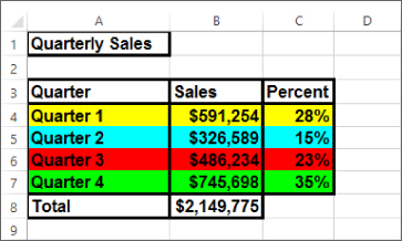
Figure 17.4

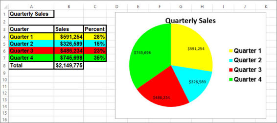
Figure 17.5

REFERENCE Please select the video for Lesson 17 online at www.wrox.com/go/excelvba24hour. You will also be able to download the code and resources for this lesson from the website.