Excel VBA 24-Hour Trainer (2015)

Part III
Beyond the Macro Recorder: Writing Your Own Code

Lesson 18
Programming PivotTables and PivotCharts

PivotTables are Excel's most powerful feature. They are an amazing tool that can summarize more than a million rows of data into concise, meaningful reports in a matter of seconds. You can format the reports in many ways, and include an interactive chart to complement the reports at no extra cost of time.

If you are not familiar with PivotTables, you are not alone. Surveys of Excel users worldwide have consistently indicated that far less than half of those surveyed said they use PivotTables, including people who use Excel throughout their entire workday. Because PivotTables are worth becoming familiar with, this lesson starts with an overview of PivotTables and PivotCharts, followed by examples of how to create and manipulate them programmatically with VBA.

Creating a PivotTable Report

Suppose you manage the clothing sales department for a national department store. You receive tens of thousands of sales records from your stores all over the country, with lists that look similar to Figure 18.1. With lists this large, it's impossible to gain any meaningful insight into trends or marketing opportunities unless you can organize the data in a summarized fashion.

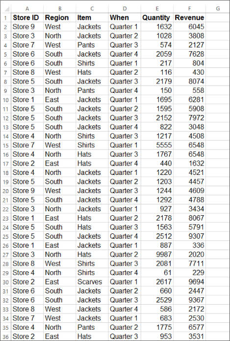
Figure 18.1

If you select a single cell anywhere in the list, such as cell E7, which is selected in Figure 18.2, you can create a PivotTable by selecting the Insert tab and clicking the PivotTable icon. The Create PivotTable dialog box appears with the Table/Range field already filled in, as shown in Figure 18.3. I chose to keep the PivotTable on the same worksheet as the source data, and for the PivotTable's top-left corner to occupy cell H4.

NOTE When placing a PivotTable on the same worksheet alongside the source table, it's best to have at least one empty column between the source table and your PivotTable. It's also a good idea to leave a few empty rows above the PivotTable to make room for the Filters area (what was called the Page area in Excel version 2003).

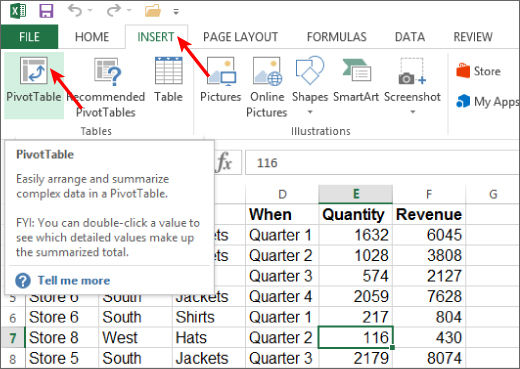
Figure 18.2

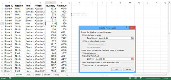
Figure 18.3

Using Excel version 2013, when you click OK you see an image similar to Figure 18.4, with the representation of where the PivotTable will be, and the Field List at the right.

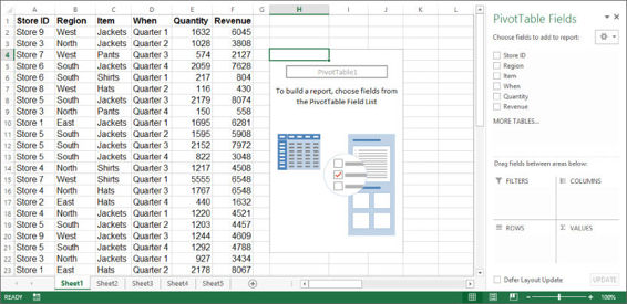
Figure 18.4

To create a PivotTable, complete the following steps:

1. Drag the Item field name from the Choose Fields to Add to Report pane down to the Filters pane.

2. Drag the Region field name from the Choose Fields to Add to Report pane down to the Rows pane.

3. Drag the Store ID field name from the Choose Fields to Add to Report pane down to the Rows pane, below the Region field name.

4. Drag the When field name from the Choose Fields to Add to Report pane down to the Columns pane.

5. Drag the Revenue field name from the Choose Fields to Add to Report pane down to the Values pane.

Your worksheet should look similar to Figure 18.5, with a PivotTable that shows the summary of Revenue by Quarter for each Region, with each Region showing the detail of its stores' activities. The source list could have been more than a million rows deep, and the process would still have taken Excel only a couple of moments to produce the PivotTable report.

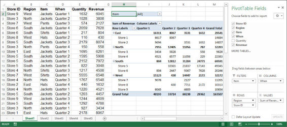
Figure 18.5

Hiding the PivotTable Field List

For now, you are done with the PivotTable Field List, so to clear it off your screen, you can click the X close button on its title bar, click its Ribbon icon on the PivotTable Tools Option tab, or you can right-click anywhere on the PivotTable area and select Hide Field List, as shown in Figure 18.6. When you want to see the Field List again, click the Field List Ribbon icon, or right-click anywhere on the PivotTable again and select Show Field List.

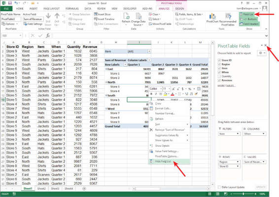
Figure 18.6

Above the PivotTable's report area, you see a small filter-looking icon in cell I2 (see Figure 18.8), in what is called the Filters area. The Item field name was dragged to that area in Step 1 of the process that created this PivotTable. If you click the filter icon, you'll see a unique list of clothing items, of which you can select one or several to have the PivotTable show only the data relating to the item(s) you select. In Figure 18.7, I selected the Hats item, and in Figure 18.8, you can see how the PivotTable adjusts itself to show only the columns and rows where data is present for the sale of hats.

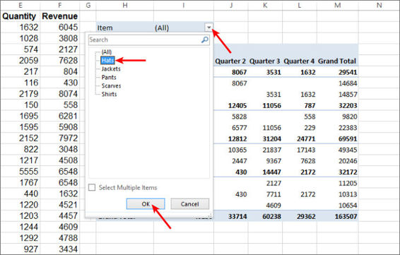
Figure 18.7

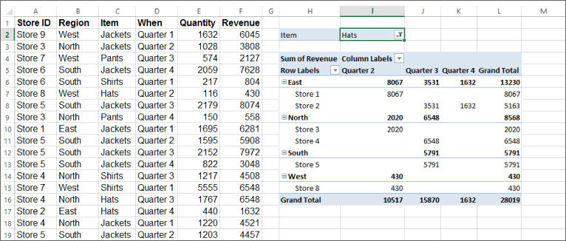
Figure 18.8

Formatting Numbers in the Values Area

You can see that the numbers in the PivotTable's Values area are unformatted. As an example of formatting them as Currency, right-click any cell in the Values area and select Value Field Settings, as indicated in Figure 18.9. In the Value Field Settings dialog box, click the Number Format button, as shown in Figure 18.10.

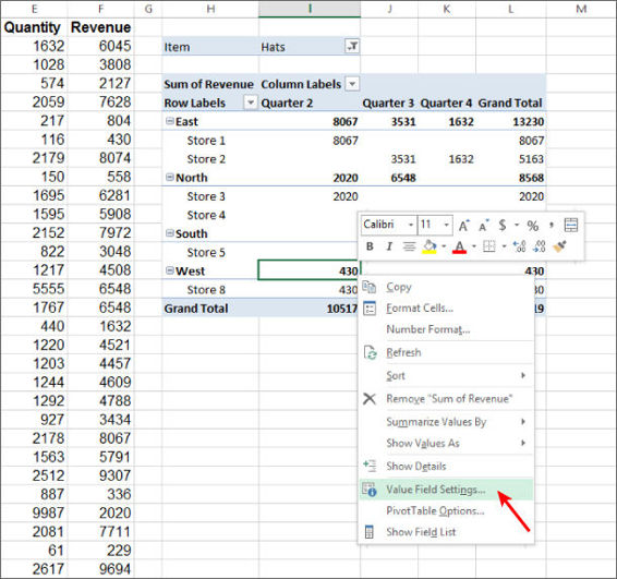
Figure 18.9

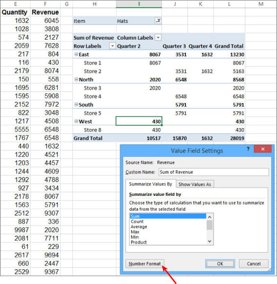
Figure 18.10

The familiar Format Cells dialog box appears. In Figure 18.11, I selected Currency with the dollar sign symbol and no decimal places. After you click OK in the Format Cells dialog box, you then need to click OK in the Value Field Settings dialog box, as shown in Figure 18.12.

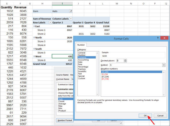
Figure 18.11

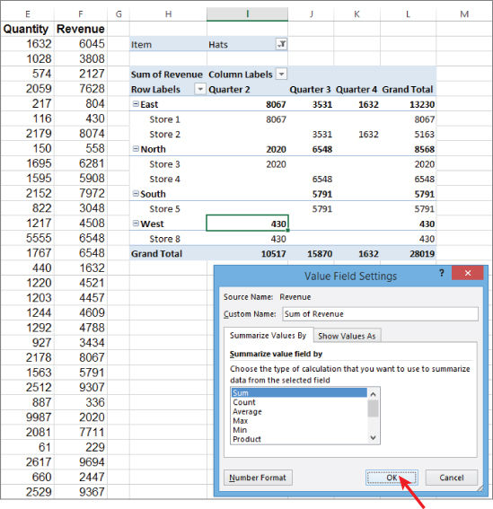
Figure 18.12

The cells in the Values area are now formatted as Currency. Recall that earlier, the Item named Hats was selected in the Filters area. Go ahead and click the filter icon in cell I2, select the All item, and click OK, as indicated in Figure 18.13. The PivotTable report is now fully displayed with all the Values area cells formatted as Currency, including the cells that had been hidden while the Hats item was filtered.

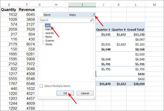
Figure 18.13

Pivoting Your Data

One of the most attractive features of a PivotTable is its ability to display the same data in whatever row-and-column arrangement of your field names that you prefer. Just as the essence of a pivot is to allow for the rotation or maneuver from a central point, you can rearrange your source data by varying the location of your field names in the row and column areas of your PivotTable.

For example, because you have summarized the clothing stores by Revenue for each Region by Quarter, you now want to look at the Quantity of each Item that was sold by Region. Reopen the PivotTable Field List and pivot your data by dragging the Item field name out of the Filters pane and into the Row Labels pane. Relocate the Region field into the Columns pane. Finally, in the Choose Fields To Add To Report pane, deselect Revenue and select Quantity. Your new PivotTable report looks like Figure 18.14.

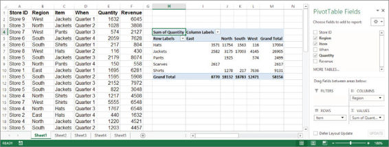
Figure 18.14

Creating a PivotChart

Creating a PivotChart is very easy, using either of two methods. With one method you create the chart right from the start, when you first indicate to Excel that you want to create a new PivotTable. With the other method you create a PivotChart after you have already created a PivotTable.

In Excel version 2010—shown in Figure 18.15—you can click the arrow on the lower half of the PivotTable icon on the Ribbon's Insert tab, where an option is there for you to select PivotChart. If you want a PivotChart with your new PivotTable, just select the PivotChart option, and a PivotChart is created as you build your PivotTable in the PivotTable Field List.

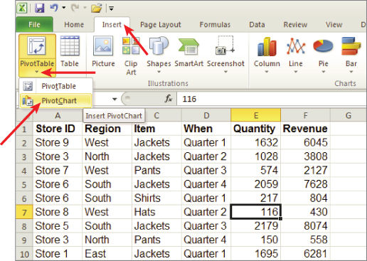
Figure 18.15

To create a PivotChart as you create a new PivotTable in version 2013, from the Insert tab on the Ribbon, click the down arrow on the PivotChart icon in the Charts section. Select PivotChart & PivotTable, as shown in Figure 18.16.

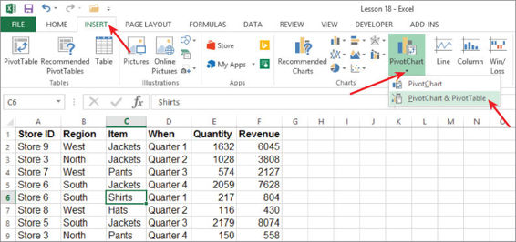
Figure 18.16

If you create a PivotTable and later decide you'd like a PivotChart to go along with it, you can start by selecting any cell in the PivotTable. In Excel version 2010, click the Options tab in the PivotTable Tools section of the Ribbon, and click the PivotChart icon, as shown in Figure 18.17. In version 2013, click the Analyze tab in the PivotTable Tools section of the Ribbon, and click the PivotChart icon, as shown in Figure 18.18.

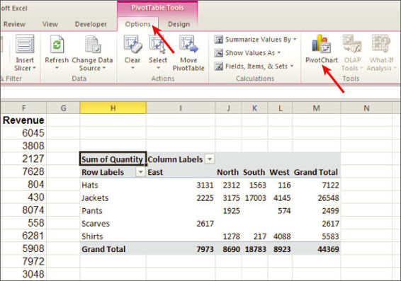
Figure 18.17

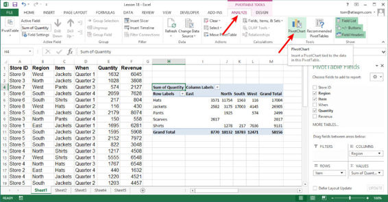
Figure 18.18

The Insert Chart dialog box opens, and you select your preferred chart type. Figure 18.19 shows the result after I selected the Clustered Column chart type and clicked OK. The result is a PivotChart tied to the PivotTable as shown in Figure 18.20.

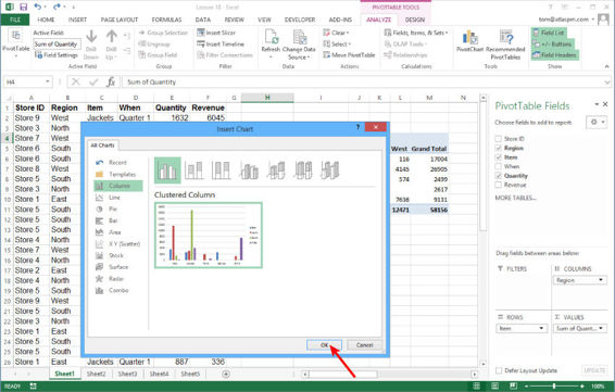
Figure 18.19

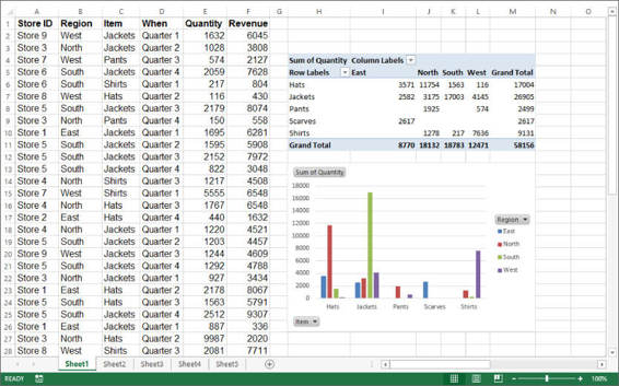
Figure 18.20

As you can see, when it comes to PivotCharts, Excel does almost all the grunt work for you. All you need to do is tell Excel that you want a PivotChart and what type of chart you want, and your chart is produced with its accompanying PivotTable.

NOTE There is a lot more you can do with PivotCharts and PivotTables; like many other topics, it's one that can fill an entire book. My objective so far in the lesson is to cover the basics of creating and working with PivotTables as a foundation for the VBA examples in the next sections.

PivotCharts are great—they are equipped with Field buttons so you can choose which items in which fields you want to see. Whatever field setting you select on a PivotChart makes the same change to its PivotTable. The following macro toggles between showing and hiding the Field buttons on your PivotChart:

Sub ShowHidePivotChartFieldButtons()

ActiveSheet.ChartObjects(1).Activate

With ActiveChart

.HasPivotFields = Not .HasPivotFields

End With

Range("A1").Select

End Sub

Understanding PivotCaches

A PivotCache is an object that you do not see, because it is working behind the scenes when a new PivotTable is created directly from the source data. The PivotCache is a container that holds a static copy of the source data in memory.

PivotTables do not summarize data directly from the source data, but rather from the PivotCache that memorized a snapshot of the data. That is why, in the native Excel environment not enhanced with VBA, if you change a piece of existing data in the source data range, the PivotTable report does not reflect that change until you refresh the PivotTable.

Figure 18.21 shows the Refresh menu item when you right-click a cell that is part of a PivotTable. The Refresh button actually refreshes the PivotCache.

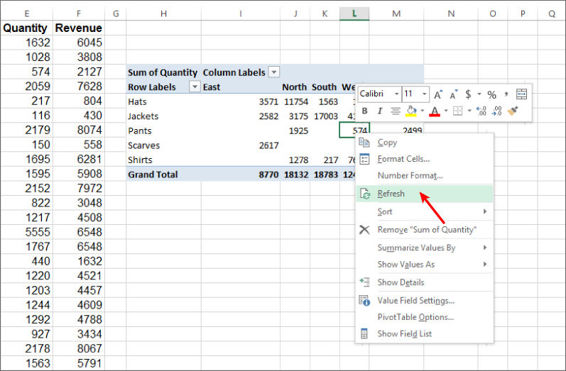
Figure 18.21

The PivotCache, though not seen, maintains the source data beforehand in a static go-to container. Keeping the data in PivotCache memory makes pivoting and recalculations a snap, but the downside is extra workbook size and less memory for other tasks.

When you create a PivotTable manually, Excel does not bother you with the PivotCache details. If you were to create a PivotTable in VBA, you'd need to address the PivotCache issue in code. Suppose you are creating a new PivotTable based on the original source data that has been shown in this lesson. Your first step would be to program VBA to tell Excel four pieces of information:

1. You want to add a PivotCache to the workbook.

2. The location of the source data.

3. Based on items 1 and 2, create the PivotTable.

4. Specify where the PivotTable will be placed.

Assuming that the worksheet holding the source data is the active sheet, and that you want the PivotTable to be located next to the source data, the following macro would handle all those instructions:

Sub CreatePivot()

ThisWorkbook.PivotCaches.Add _

(SourceType:=xlDatabase, _

SourceData:=Range("A1").CurrentRegion).CreatePivotTable _

TableDestination:="R4C" & Range("A1").CurrentRegion.Columns.Count + 2

End Sub

NOTE The notation "R4C" & Range("A1").CurrentRegion.Columns.Count + 2 is translated as the worksheet cell that is on row 4 of the column that is two columns to the right of the last column in the source range. Recall from earlier in the lesson that I recommend placing the top-left corner of the PivotTable on row 4, and with an empty column separating the source data and the new PivotTable.

The result you get is a PivotTable, but you'd never know by its appearance at the moment—a curious range of four cells look as if they were formatted for thin borders. In this example, the four cells are in range H4:I5, as shown in Figure 18.22.

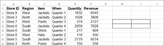
Figure 18.22

The macro is just getting started, but I wanted to show you in slow motion what is taking place under the radar when a new PivotTable is created. Actually, with the preceding macro executed, you could select one of those four cells and the PivotTable Field List would appear, inviting you to drag fields to your desired location, as shown in Figure 18.23. In Figure 18.24, the Item field was moved to the Rows area and the When field was moved to the Columns area.

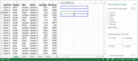
Figure 18.23

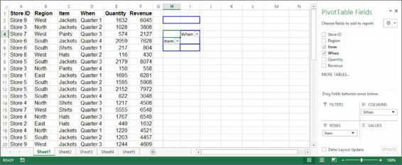
Figure 18.24

When a numerical field is moved into the Values area, the PivotTable becomes more recognizable. For example, Figure 18.25 shows the result of moving the Revenue field into the Values area.

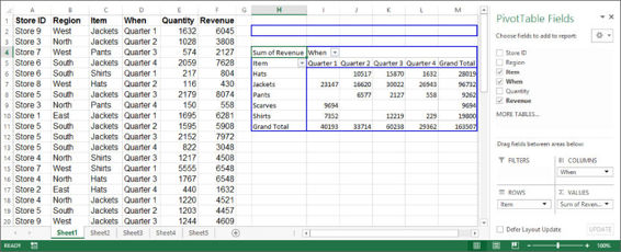
Figure 18.25

NOTE If you want your PivotTable's PivotCache to refresh automatically when a cell in your source list changes, the following Worksheet_Change event handles that. Note that the code uses the PivotTable's Index property for the first or only PivotTable on the worksheet to be refreshed:

Private Sub Worksheet_Change(ByVal Target As Range)

If Intersect(Target, Range("A1").CurrentRegion) Is Nothing _

Or Target.Cells.Count > 1 Then Exit Sub

ActiveSheet.PivotTables(1).PivotCache.Refresh

End Sub

Manipulating PivotFields in VBA

PivotFields are the row and column areas that you place your field names into, depending on how you want the PivotTable to display your data. The following pieces of VBA code perform the placement of PivotFields as they were for the PivotTable that you created manually earlier in the lesson. Two fields (Region and Store ID) are placed as row labels, and one field (When) is placed as a column label. The Revenue field is placed in the Values area, and the Filters area is populated by the Items field:

With ActiveSheet.PivotTables(1)

'First (outer) row field.

With .PivotFields("Region")

.Orientation = xlRowField

.Position = 1

End With

'Second (inner) row field.

With .PivotFields("Store ID")

.Orientation = xlRowField

.Position = 2

End With

'Column field.

With .PivotFields("When")

.Orientation = xlColumnField

.Position = 1

End With

'Filters area.

With .PivotFields("Item")

.Orientation = xlPageField

.Position = 1

End With

'Revenue in the Values field.

.AddDataField ActiveSheet.PivotTables(1).PivotFields("Revenue"), _

"Sum of Amount", xlSum

End With

NOTE Be sure to name your PivotFields correctly! They must be spelled the same way in your code as they are in the header cells of your source list. If you misspell the field names in your code, VBA lets you know with a runtime error because the field names you're instructing VBA to manipulate do not exist.

Manipulating PivotItems with VBA

PivotItems are programmable in PivotTables, and as an example, you can arrange to see just one particular PivotItem in a field. In a PivotTable that you created earlier in the lesson, you added a Region field. Suppose you want to see activity only for the North PivotItem and hide the South, East, and West PivotItems. The following macro accomplishes that:

Sub ShowSingleItem()

Dim objPivotField As PivotField

Dim objPivotItem As PivotItem

Set objPivotField = _

ActiveSheet.PivotTables(1).PivotFields(Index:="Region")

For Each objPivotItem In objPivotField.PivotItems

If objPivotItem.Name = "North" Then

objPivotItem.Visible = True

Else

objPivotItem.Visible = False

End If

Next objPivotItem

End Sub

The following macro shows all the PivotItems:

Sub ShowAllItems()

Dim objPivotField As PivotField

Dim objPivotItem As PivotItem

Set objPivotField = _

ActiveSheet.PivotTables(1).PivotFields(Index:="Region")

For Each objPivotItem In objPivotField.PivotItems

objPivotItem.Visible = True

Next objPivotItem

End Sub

Creating a PivotTables Collection

PivotTables are objects for which there is a Collection object, just as there is for worksheets and workbooks. As you might guess, the name of the Collection object for PivotTables is PivotTables, and you can loop through every PivotTable on a worksheet or throughout the workbook if you need to.

For example, if you have more than one PivotTable on a worksheet and they are tied to the same source list that starts in cell A1, this Worksheet_Change event refreshes all PivotTables on that worksheet automatically when the source data is changed:

Private Sub Worksheet_Change(ByVal Target As Range)

If Intersect(Target, Range("A1").CurrentRegion) Is Nothing _

Or Target.Cells.Count > 1 Then Exit Sub

Dim PT As PivotTable

For Each PT In ActiveSheet.PivotTables

PT.RefreshTable

Next PT

End Sub

Suppose you have several PivotTables on many different worksheets and you want to be confident that every PivotTable displays the current data from its respective source lists. The following Workbook_Openprocedure refreshes every PivotTable in the workbook when the workbook opens:

Private Sub Workbook_Open()

Dim wks As Worksheet, PT As PivotTable

For Each wks In Worksheets

For Each PT In wks.PivotTables

PT.RefreshTable

Next PT

Next wks

End Sub

NOTE You can avoid looping through all your PivotTables by using VBA's RefreshAll method to refresh all PivotTables at once. The single line of code would be ActiveWorkbook.RefreshAll. Just be aware that the RefreshAll method also refreshes all external data ranges, such as web queries, for the specified workbook.

You might need to delete all the PivotTables on a worksheet. When you delete a PivotTable, what you are really doing is clearing the cells that are occupied by the PivotTable. The following macro deletes all the PivotTables on the active worksheet:

Sub DeleteAllPivotTablest()

Dim objPT As PivotTable, iCount As Integer

For iCount = ActiveSheet.PivotTables.Count To 1 Step -1

Set objPT = ActiveSheet.PivotTables(iCount)

objPT.PivotSelect ""

Selection.Clear

Next iCount

End Sub

Try It

In this lesson, you write a macro that adds a PivotChart to accompany an existing PivotTable. Your new PivotChart will be located below the PivotTable on that same worksheet.

Lesson Requirements

Your worksheet contains a list of source data, and you already have a PivotTable on your worksheet, as shown in Figure 18.26. To get the sample workbook, you can download Lesson 18 from the book's website at www.wrox.com/go/excelvba24hour.

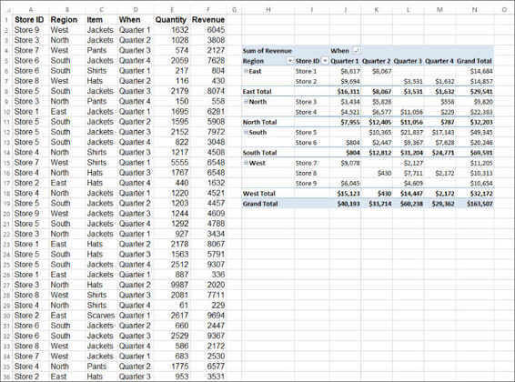
Figure 18.26

Step-by-Step

1. Activate the worksheet that contains the source data list and PivotTable.

2. Press Alt+F11 to go to the Visual Basic Editor.

3. From the menu bar, click InsertModule.

4. In the new module, type Sub CreatePivotChart and press Enter. VBA produces the following lines of code for you:

5. Sub CreatePivotChart()

End Sub

5. Turn off ScreenUpdating to help your macro run faster by not refreshing the screen as objects in the code are created and manipulated:

Application.ScreenUpdating = False

6. Declare an Object variable for the existing PivotTable:

Dim objPT As PivotTable

7. Set the Object variable for the first (index #1) PivotTable:

Set objPT = ActiveSheet.PivotTables(1)

8. Select the PivotTable:

objPT.PivotSelect ""

9. Add the chart:

Charts.Add

10.Place the chart onto the PivotTable's worksheet:

11. ActiveChart.Location Where:=xlLocationAsObject, _

Name:=objPT.Parent.Name

11.Position the PivotChart so its top-left corner occupies cell H23, a few rows below the PivotTable:

12. ActiveChart.Parent.Left = Range("H23").Left

ActiveChart.Parent.Top = Range("H23").Top

12.Deselect the PivotChart:

Range("A1").Select

13.Turn on ScreenUpdating:

Application.ScreenUpdating = True

14.When you complete the macro, it looks as follows:

15. Sub CreatePivotChart()

16. 'Turn off ScreenUpdating.

17. Application.ScreenUpdating = False

18. 'Declare an Object variable for the existing PivotTable.

19. Dim objPT As PivotTable

20. 'Set the Object variable for the first (index #1) PivotTable.

21. Set objPT = ActiveSheet.PivotTables(1)

22. 'Select the PivotTable.

23. objPT.PivotSelect ""

24. 'Add the chart.

25. Charts.Add

26. 'Place it on the PivotTable's worksheet.

27. ActiveChart.Location Where:=xlLocationAsObject, _

28. Name:=objPT.Parent.Name

29. 'Position the PivotChart so its top left corner

30. 'occupies cell H23, a few rows below the PivotTable.

31. ActiveChart.Parent.Left = Range("H23").Left

32. ActiveChart.Parent.Top = Range("H23").Top

33. 'Deselect the PivotChart.

34. Range("A1").Select

35. 'Turn on ScreenUpdating.

36. Application.ScreenUpdating = True

End Sub

15.Press Alt+Q to return to your worksheet and test your macro. Figure 18.27 shows what the worksheet should look like with the PivotChart added, right where it was specified in VBA.

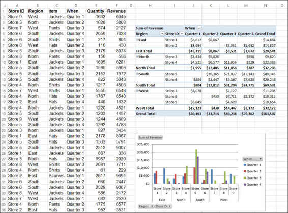
Figure 18.27

REFERENCE Please select the video for Lesson 18 at www.wrox.com/go/excelvba24hour. You will also be able to download the code and resources for this lesson from the website.