Excel VBA 24-Hour Trainer (2015)

Part IV
Advanced Programming Techniques

Lesson 28
Impressing Your Boss (or at Least Your Friends)

Microsoft estimates that Excel is loaded onto some 600 million computers worldwide. One trait all Excel users have in common is that no one knows all there is to know about Excel. The power and diversity of Excel's native capabilities alone are more than enough to master. With VBA for Excel—each new version having more features than the one before—the capabilities for performance, object programming, and data management are virtually limitless.

The theme of this lesson is to show a variety of examples of what Excel can achieve with VBA. I encourage you to continue advancing your VBA skills after reading this book, and hopefully, being inspired by the more advanced examples in this lesson.

NOTE In general, the examples in this lesson are a bit more advanced than what you've seen in the book so far. Be sure to watch the 15 videos of advanced VBA examples that accompany this book!

Selecting Cells and Ranges

A common request I have received from Excel users is how to show the current location on a worksheet by highlighting the active cell, row, or column. It is easier to maintain your bearings in worksheets such as budgets and financial statements when a color stands out to show where you are.

Coloring the Active Cell, Row, or Column

In Figure 28.1, three examples are shown that format either the active cell only, the active cell's entire row and column, or the row and column within the active cell's current region.

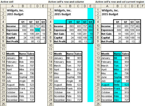
Figure 28.1

These are Worksheet_SelectionChange events. To install this behavior for a worksheet, right-click that worksheet tab, select View Code, and paste either of the following procedures (but not more than one at a time per worksheet) into the large white area that is the worksheet module. Press Alt+Q to return to the worksheet. Then, select a few cells to see the effects of the code.

To format the active cell only:

Private Sub Worksheet_SelectionChange(ByVal Target As Range)

Application.ScreenUpdating = False

Cells.Interior.ColorIndex = 0

Target.Interior.Color = vbCyan

Application.ScreenUpdating = True

End Sub

To format the entire row and column of the active cell:

Private Sub Worksheet_SelectionChange(ByVal Target As Range)

If Target.Cells.Count > 1 Then Exit Sub

Application.ScreenUpdating = False

Cells.Interior.ColorIndex = 0

With Target

.EntireColumn.Interior.Color = vbCyan

.EntireRow.Interior.Color = vbCyan

End With

Application.ScreenUpdating = True

End Sub

To format the row and column within the current region of the active cell:

Private Sub Worksheet_SelectionChange(ByVal Target As Range)

Cells.Interior.ColorIndex = 0

If IsEmpty(Target) Or Target.Cells.Count > 1 Then Exit Sub

Application.ScreenUpdating = False

With ActiveCell

Range(Cells(.Row, .CurrentRegion.Column), _

Cells(.Row, .CurrentRegion.Columns.Count + .CurrentRegion.Column - 1)) _

.Interior.Color = vbCyan

Range(Cells(.CurrentRegion.Row, .Column), _

Cells(.CurrentRegion.Rows.Count + .CurrentRegion.Row - 1, .Column)) _

.Interior.Color = vbCyan

End With

Application.ScreenUpdating = True

End Sub

Coloring the Current and Prior Selected Cells

This section explains how you can highlight not only the current cell but also the cell you selected before you selected your current cell. To make it easy to distinguish between the two cells, the currently selected cell is colored cyan, and the prior selected cell is colored magenta.

In Figure 28.2, cell C5 is the active (currently selected) cell, indicated by its cyan color when you install the following code into your workbook. You can also see its address in the address bar. Before the image of Figure 28.2 was created, cell H12 had been selected, evidenced by its magenta color.

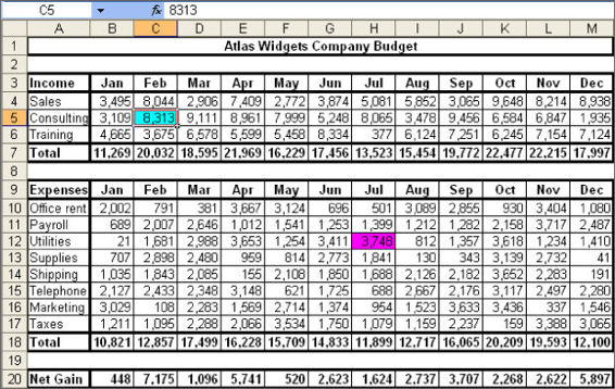
Figure 28.2

In Figure 28.3, the currently selected cell is L18, colored cyan. Now cell C5, which was selected before as seen in Figure 28.2, is colored magenta.

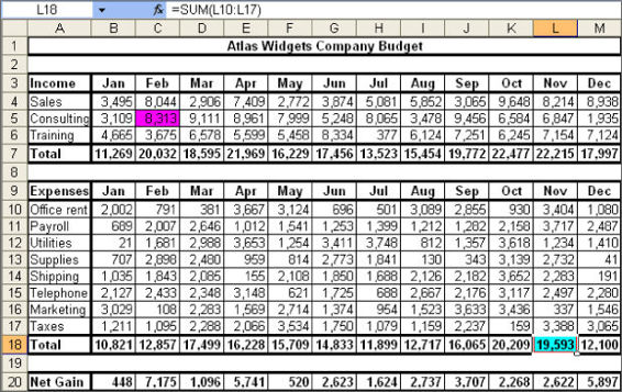
Figure 28.3

The following procedure that produces this functionality is a Selection_Change event. Place it into your worksheet module and test the code by selecting a few cells:

Private Sub Worksheet_SelectionChange(ByVal Target As Range)

Cells.Interior.ColorIndex = 0

Static PriorCell As Range

If Not PriorCell Is Nothing Then _

PriorCell.Interior.Color = vbMagenta

Target.Interior.Color = vbCyan

Set PriorCell = Target

End Sub

Filtering Dates

When it comes to filtering dates, a little VBA goes a long way in dealing with the nemesis of seemingly countless different formats in which a date can be represented in Excel. The key to filtering dates is to treat them as the numeric value they are, and to use the DateSerial function for an unambiguous date reference. No matter what the date formatting gods throw at you, the following macros filter your dates.

Filtering between Dates

On the left in Figure 28.4, dates are shown in many formats in column A. To make it more challenging, cells B2 and B3 contain the start and end date criteria that are formatted the same as only one cell in the list being filtered. The macro named FilterBetweenDates filters the dates as shown on the right in Figure 28.4.

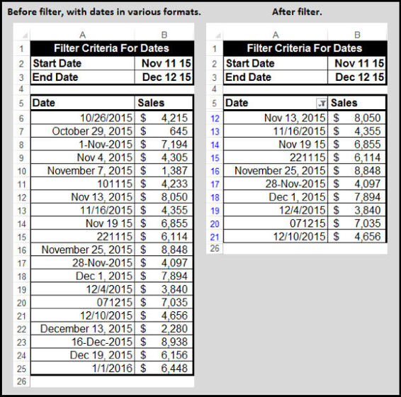
Figure 28.4

Sub FilterBetweenDates()

Application.ScreenUpdating = False

ActiveSheet.AutoFilterMode = False

Dim StartDate As Date, EndDate As Date

Dim FilterStartDate As Date, FilterEndDate As Date

Dim LastRow As Long

Dim FilterRange As Range

StartDate = Range("B2").Value

EndDate = Range("B3").Value

LastRow = _

Cells.Find(What:="*", After:=Range("A1"), _

SearchOrder:=xlByRows, SearchDirection:=xlPrevious).Row

Set FilterRange = Range("A5:A" & LastRow)

FilterStartDate = _

DateSerial(Year(StartDate), Month(StartDate), Day(StartDate) - 1)

FilterEndDate = _

DateSerial(Year(EndDate), Month(EndDate), Day(EndDate) + 1)

FilterRange.AutoFilter _

Field:=1, Criteria1:=">" & CDbl(FilterStartDate), _

Operator:=xlAnd, _

Criteria2:="<" & CDbl(FilterEndDate)

Set FilterRange = Nothing

Application.ScreenUpdating = True

End Sub

Filtering for Dates before Today's Date

The macro named FilterDateBeforeToday filters for dates before today's date. The reference to where the data table begins is the same as what is shown in Figure 28.4.

Sub FilterDateBeforeToday()

Application.ScreenUpdating = False

ActiveSheet.AutoFilterMode = False

Dim LastRow As Long, FilterRange As Range

LastRow = _

Cells.Find(What:="*", After:=Range("A1"), _

SearchOrder:=xlByRows, SearchDirection:=xlPrevious).Row

Set FilterRange = Range("A5:A" & LastRow)

FilterRange.AutoFilter Field:=1, Criteria1:="<" & CDbl(Date)

Set FilterRange = Nothing

Application.ScreenUpdating = True

End Sub

Filtering for Dates after Today's Date

The macro named FilterDateAfterToday filters for dates after today's date. The reference to where the data table begins is the same as what is shown in Figure 28.4.

Sub FilterDateAfterToday()

Application.ScreenUpdating = False

ActiveSheet.AutoFilterMode = False

Dim LastRow As Long, FilterRange As Range

LastRow = Cells.Find(What:="*", After:=Range("A1"), _

SearchOrder:=xlByRows, SearchDirection:=xlPrevious).Row

Set FilterRange = Range("A5:A" & LastRow)

FilterRange.AutoFilter Field:=1, Criteria1:=">" & CDbl(Date)

Set FilterRange = Nothing

Application.ScreenUpdating = True

End Sub

Deleting Rows for Filtered Dates More Than Three Years Ago

The macro named DeleteRows3YearsOld filters for dates that are three years ago from today's date:

Sub DeleteRows3YearsOld()

Application.ScreenUpdating = False

ActiveSheet.AutoFilterMode = False

Dim FilterRange As Range, myDate As Date

myDate = DateSerial(Year(Date) - 3, Month(Date), Day(Date))

Set FilterRange = _

Range("A5:A" & Cells(Rows.Count, 1).End(xlUp).Row)

FilterRange.AutoFilter Field:=1, Criteria1:="<" & CDbl(myDate)

On Error Resume Next

With FilterRange

.Offset(1).Resize(.Rows.Count - 1).SpecialCells(xlCellTypeVisible).EntireRow.Delete

End With

Err.Clear

Set FilterRange = Nothing

ActiveSheet.AutoFilterMode = False

Application.ScreenUpdating = True

End Sub

Setting Page Breaks for Specified Areas

If your worksheet has areas of data that you want to print on separate pages, you can establish page breaks based on a wide choice of cell properties or text values. With the following macro named PageBreakInsert, page breaks are set below each cell in column A that starts with Total, as shown in Figure 28.5.

Sub PageBreakInsert()

Cells.PageBreak = xlPageBreakNone

Dim cell As Range

For Each cell In Columns(1).SpecialCells(xlCellTypeConstants)

If Left(cell.Value, 5) = "Total" Then

With ActiveSheet

.HPageBreaks.Add Cells(cell.Row + 1, 1)

.DisplayAutomaticPageBreaks = True

End With

End If

Next cell

End Sub

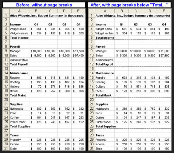
Figure 28.5

Using a Comment to Log Changes in a Cell

This section shows how you can keep a running log of changes to a cell's text. Suppose you want your employees to enter an explanation or description into a cell regarding a topic on your spreadsheet. Maybe there's a new product being developed and you'll utilize cell A1 for team members to enter their ideas during production. You want to keep a record of everything entered, without burdening anyone with how to edit existing text or how to add a new comment to a cell.

In Figure 28.6, new entries are made into cell A1 on an ongoing basis. Although each new entry overrides preexisting text, the following procedure captures all the text that has been previously entered. There's also a date and time stamp for each new entry, and an empty line between entries in the comment for readability. This is a Worksheet_Change procedure, which goes into your worksheet module:

Private Sub Worksheet_Change(ByVal Target As Range)

With Target

If .Address <> "$A$1" Then Exit Sub

If IsEmpty(Target) Then Exit Sub

Dim strNewText$, strCommentOld$, strCommentNew$

strNewText = .Text

If Not .Comment Is Nothing Then

strCommentOld = .Comment.Text & Chr(10) & Chr(10)

Else

strCommentOld = ""

End If

On Error Resume Next

.Comment.Delete

Err.Clear

.AddComment

.Comment.Visible = False

.Comment.Text Text:=strCommentOld & _

Format(VBA.Now, "MM/DD/YYYY at h:MM AM/PM") & Chr(10) & strNewText

.Comment.Shape.TextFrame.AutoSize = True

End With

End Sub

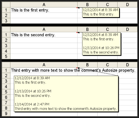
Figure 28.6

Using the Windows API with VBA

With the Windows API (application programming interface), you can program Windows objects that are not specific to Excel. Examples of Windows objects are the browser window, the status bar, and, as the following two macros demonstrate, the clipboard and the recycle bin.

NOTE Starting in version 2010 and continuing with version 2013, you can install Excel as a 64-bit application if you are running a 64-bit version of Windows. Many Excel users, including myself, prefer the 32-bit version because it provides all the power needed while supporting ActiveX controls. Other Excel users prefer the 64-bit version if they work with enormous amounts of data.

The examples in this section are 32-bit API declarations and might not work in 64-bit versions. This raises the larger point that if your workbooks will be shared among both versions, your code must be compatible for either version to run it.

In most cases, your 32-bit API declarations will be compatible with 64-bit versions by inserting PtrSafe after the Declare key word. Fortunately, you don't need to create two workbooks, but you do need to declare your API functions twice, using an If…Then…Else statement to establish the API calls for both versions. Lesson 32 shows this construction for an example that opens an Access database file.

The introduction of 64-bit Excel is relatively new, and it can be difficult to remember the nuances, as well as the syntaxes. For example, versions of Excel before 2010, including version 2007, do not recognize the PtrSafe keyword. For an excellent resource about this topic, Jan Karel Pieterse of JKP Application Development Services (http://www.jkp-ads.com) maintains an ongoing list of proper syntax for API declarations in 32-bit and 64-bit versions. You can visit Jan Karel's web page at http://www.jkp-ads.com/articles/apideclarations.asp.

Clearing the Clipboard

The Windows clipboard is a temporary storage area for information that you have copied or moved from one place and plan to use somewhere else. You cannot see or touch the clipboard but you can work with it to copy, cut, paste, and clear data.

You can copy some 30 types of data onto your clipboard beyond just text and formulas, such as graphics, charts, and hyperlinks. To truly empty the clipboard requires more than just pressing the Esc key or executing the VBA statement Application.CutCopyMode = False.

With the Windows API, the macro named ClearClipboard clears all data types on your clipboard. The API function calls that precede the macro go at the top of your module, above and outside of the macro itself:

Public Declare Function OpenClipboard Lib "user32" _

(ByVal hwnd As Long) As Long

Public Declare Function CloseClipboard Lib "user32" () As Long

Public Declare Function EmptyClipboard Lib "user32" () As Long

Sub ClearClipboard()

OpenClipboard (0&)

EmptyClipboard

CloseClipboard

End Sub

Emptying the Recycle Bin

This macro named RecycleBinEmpty empties the recycle bin. The API function call named EmptyRecycleBin goes at the top of your module, above and outside of the macro itself:

Declare Function EmptyRecycleBin _

Lib "shell32.dll" Alias "SHEmptyRecycleBinA" _

(ByVal hwnd As Long, _

ByVal pszRootPath As String, _

ByVal dwFlags As Long) As Long

Sub RecycleBinEmpty()

Dim rbEmpty As Long

rbEmpty = EmptyRecycleBin(0&, vbNullString, 1&)

End Sub

Scheduling Your Workbook for Suicide

If you have developed a workbook that you want to self-expire by a certain date, such as a demonstration model or one that contains information or usefulness that will be outdated, you can program the workbook to delete itself. In this example, the workbook's suicide date is scheduled for December 31, 2015.

In actual practice, you might want to have a message box—say, seven days prior to the suicide date—to let the workbook's users know what to expect on the upcoming date of demise. You would also lock and password-protect the Visual Basic Editor to reduce the chance for the code to be altered or deleted.

Please be careful when employing this code. When it executes, the recycle bin is bypassed, so your workbook is gone forever. The code goes into the workbook module and is evaluated every time the workbook opens.

Sub Workbook_Open()

If Date <= #12/31/2015# Then Exit Sub

MsgBox "This workbook has expired.", vbExclamation, "Goodbye."

With ThisWorkbook

.Saved = True

.ChangeFileAccess xlReadOnly

Kill .FullName

.Close False

End With

End Sub

Try It

For this lesson, you establish data validation in a cell, for which the allowable entries are the items in a custom list. Data validation by itself cannot directly access custom lists, but with VBA you can establish data validation to access a custom list in your Excel application.

Custom lists are identified in VBA by their index number. In the collection of custom lists on my computer, a fifth one will be added and used for this example.

Lesson Requirements

If you have not already done so, please establish a fifth custom list in your Excel application. You probably already have four that came with your Excel version. Otherwise, you will need to edit the number 5 in Step 11 to a lower number representing an existing custom list that you prefer to use.

To get the sample workbook, you can download Lesson 28 from the book's website at www.wrox.com/go/excelvba24hour.

Hints

The macro for this example uses the fifth custom list in an Excel application. If you are not familiar with custom lists, Steps 2 to 6 explain how to add a custom list.

You can add, delete, or edit the items in your custom list. When you run the macro again, those changes show in the data validation drop-down list.

Step-by-Step

1. Start by opening a new workbook.

2. If you are not familiar with adding a custom list, click the File tab and select the Options menu item as shown in Figure 28.7.

3. In the Excel Options dialog box, click the Advanced menu item. Scroll down to the General section, and click the Edit Custom Lists button as shown in Figure 28.8.

4. Click NEW LIST in the list box at the left, enter your list items in the list box at the right, and click Add as shown in Figure 28.9.

5. You see your new list of items in the list box at the left. Click OK as shown in Figure 28.10.

6. Click OK to exit the Excel Options dialog box as shown in Figure 28.11.

7. Press Alt+F11 to go to the Visual Basic Editor.

8. From the VBE menu bar, click Insert Module.

9. In the module you just created, type Sub CustomListDV and press Enter. VBA automatically places a pair of empty parentheses at the end of the Sub line, followed by an empty line, and the End Sub line below that. Your macro should look like this so far:

10. Sub CustomListDV()

End Sub

10.Declare a String type variable for custom items to be allowed by data validation, an Integer type variable to iterate through the array of items in your custom list, and a Variant type for the array itself:

11. Dim strCustomItems As String, intArray As Integer

Dim myCustomList As Variant

11.Identify your custom list by its index number:

myCustomList = Application.GetCustomListContents(5)

12.Open a For…Next loop to iterate through each element in your custom list:

For intArray = LBound(myCustomList) To UBound(myCustomList)

13.Build the string for each custom item, separated by a comma:

strCustomItems = strCustomItems & myCustomList(intArray) & ","

14.Continue the loop until completion:

Next intArray

15.Delete the trailing comma after the last custom list item:

strCustomItems = Mid(strCustomItems, 1, Len(strCustomItems) - 1)

16.Establish data validation for the cell of interest:

17. With Range("B7").Validation

18. 'Delete the existing data validation.

19. .Delete

20. 'Add the string of items from your custom list.

21. .Add Type:=xlValidateList, _

22. AlertStyle:=xlValidAlertStop, _

23. Operator:=xlBetween, _

24. Formula1:=strCustomItems

25. 'Error title if an invalid entry is attempted.

26. .ErrorTitle = "Invalid entry !"

27. 'Error message if an invalid entry is attempted.

28. 'Note the ascii 10 character which is for a line break.

29. .ErrorMessage = "Please enter an item" & Chr(10) & _

30. "from the drop-down list."

31. 'Show the error icon in the message for invalid entries.

32. .ShowError = True

33. End With

End Sub

17.With your macro completed, press Alt+Q to return to the worksheet. To test the macro, press Alt+F8 to show the Macro dialog box. Select the macro named CustomListDV and click Run. Here is what the macro looks like in its entirety:

18. Sub CustomListDV()

19. 'Declare variables:

20. 'Custom items to be allowed by data validation,

21. 'a counter for the array elements in the custom list,

22. 'and your custom list.

23. Dim strCustomItems As String, intArray As Integer

24. Dim myCustomList As Variant

25. 'Identify your custom list by its index number.

26. myCustomList = Application.GetCustomListContents(5)

27. 'Loop through each element in your custom list.

28. For intArray = LBound(myCustomList) To UBound(myCustomList)

29. 'Build the string for each custom item, separated by a comma.

30. strCustomItems = strCustomItems & myCustomList(intArray) & ","

31. 'Continue the loop until completion.

32. Next intArray

33. 'Delete the trailing comma after the last custom list item.

34. strCustomItems = Mid(strCustomItems, 1, Len(strCustomItems) - 1)

35. 'Establish data validation for the cell(s) of interest.

36. With Range("B7").Validation

37. 'Delete the existing data validation.

38. .Delete

39. 'Add the string of items from your custom list.

40. .Add Type:=xlValidateList, _

41. AlertStyle:=xlValidAlertStop, _

42. Operator:=xlBetween, _

43. Formula1:=strCustomItems

44. 'Error title if an invalid entry is attempted.

45. .ErrorTitle = "Invalid entry !"

46. 'Error message if an invalid entry is attempted.

47. 'Note the ascii 10 character which is for a line break.

48. .ErrorMessage = "Please enter an item" & Chr(10) & _

49. "from the drop-down list."

50. 'Show the error icon in the message for invalid entries.

51. .ShowError = True

52. End With

End Sub

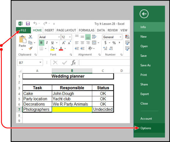
Figure 28.7

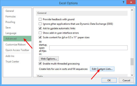
Figure 28.8

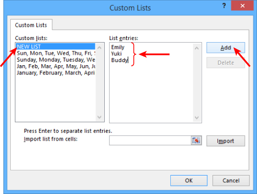
Figure 28.9

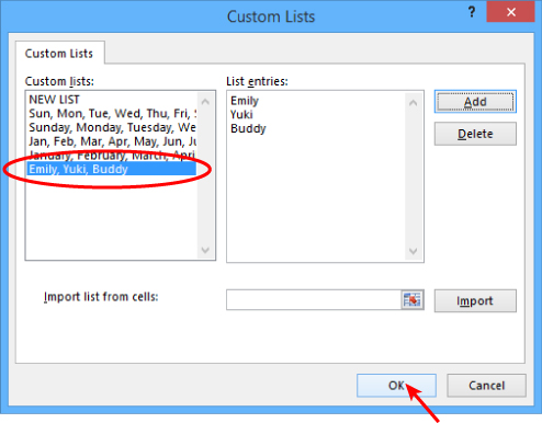
Figure 28.10

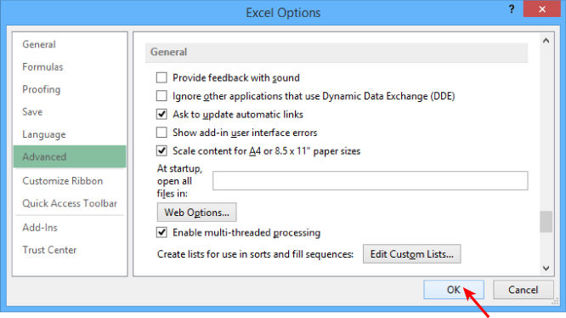
Figure 28.11

REFERENCE Please select the video for Lesson 28 online at www.wrox.com/go/excelvba24hour. You will also be able to download the code and resources for this lesson from the website.