Cython (2015)
Chapter 9. Cython Profiling Tools
I’ve never been a good estimator of how long things are going to take.
— D. Knuth
If you optimize everything, you will always be unhappy.
— D. Knuth
Cython lets us easily move across the boundary between Python and C. Rather than taking this as license to bring in C code wherever we like, however, we should consider just how much C we want to mix with our Python. When we are wrapping a library, the answer is usually determined for us: we need enough C to wrap our library, and enough Python to make it nice to use. When we’re using Cython to speed up a Python module, though, the answer is much less clear. Our goal is to bring in enough C code to get the best results for our efforts, and no more. Cython has tools that can help us find this sweet spot, which we cover in this chapter.
Cython Runtime Profiling
When we are optimizing Cython code, the principles, guidelines, and examples in the rest of this book help us answer the how. But sometimes the challenge is determining what code needs to change in the first place. I strongly recommend that, rather than looking at code and guessing, we use profiling tools to provide data to quantify our programs’ performance.
Python users are spoiled when it comes to profiling tools. The built-in profile module (and its faster C implementation, cProfile) makes runtime profiling easy. On top of that, the IPython interpreter makes profiling nearly effortless with the %timeit and %run magic commands, which support profiling small statements and entire programs, respectively.
These profiling tools work without modification on pure-Python code. But when Python code calls into C code in an extension module or in a separate library, these profiling tools cannot cross the language boundary. All profiling information for C-level operations is lost.
Cython addresses this limitation: it can generate C code that plays nicely with these runtime profiling tools, fooling them into thinking that C-level calls are regular Python calls.
For instance, let’s start with a pure-Python version of the integration example from Chapter 3:[16]
def integrate(a, b, f, N=2000):
dx = (b-a)/N
s = 0.0
for i inrange(N):
s += f(a+i*dx)
return s * dx
We will use runtime profiling to help improve integrate’s performance.
First, we create a main.py Python script to drive integrate:
from integrate import integrate
from math import pi, sin
def sin2(x):
return sin(x)**2
def main():
a, b = 0.0, 2.0 * pi
return integrate(a, b, sin2, N=400000)
To profile our function, we can use cProfile in the script itself, sorting by the internal time spent in each function:
if __name__ == '__main__':
import cProfile
cProfile.run('main()', sort='time')
Running our script gives the following output:
$ python main.py
800005 function calls in 0.394 seconds
Ordered by: internal time
ncalls tottime percall cumtime percall filename:lineno(function)
1 0.189 0.189 0.394 0.394 integrate.py:2(integrate)
400000 0.140 0.000 0.188 0.000 main.py:4(sin2)
400000 0.048 0.000 0.048 0.000 {math.sin}
1 0.017 0.017 0.017 0.017 {range}
1 0.000 0.000 0.394 0.394 main.py:7(main)
1 0.000 0.000 0.394 0.394 <string>:1(<module>)
...
This output is generated by the cProfile.run call. Each row in the table is the collected runtime data for a function called in the course of running our program. The ncalls column is, unsurprisingly, the number of times that function or method was called. The tottime column is the total time spent in the function, not including time spent in called functions. This is the column used to sort the output, and it usually provides the most useful information. The first percall column is tottime divided by ncalls. The cumtime column is the total time spent in this functionincluding time spent in called functions, and the second percall column is cumtime divided by ncalls. The last column is the name of the module, the line number, and the function name for the table row.
As expected, most time is spent in the integrate function, followed by our sin2 function.
Let’s convert integrate.py to an extension module, integrate.pyx. For now, we change only the filename without changing the contents. Doing so requires us to compile our extension module before using it in main.py.
We can use pyximport to compile at import time; at the top of main.py, we add this one line before importing integrate:
import pyximport; pyximport.install()
from integrate import integrate
# ...
Running our script again compiles the extension module automatically and generates the profiling output for our Cythonized version of integrate:
$ python main.py
800004 function calls in 0.327 seconds
Ordered by: internal time
ncalls tottime percall cumtime percall filename:lineno(function)
1 0.141 0.141 0.327 0.327 {integrate.integrate}
400000 0.138 0.000 0.185 0.000 main.py:5(sin2)
400000 0.047 0.000 0.047 0.000 {math.sin}
1 0.000 0.000 0.327 0.327 main.py:8(main)
1 0.000 0.000 0.327 0.327 <string>:1(<module>)
...
Just compiling our module gives us an overall 17 percent performance boost, and improves integrate’s performance by about 25 percent. We will see just how much faster we can make integrate by using more Cython features.
Let’s add static type information to integrate to generate more efficient code:
def integrate(double a, double b, f, int N=2000):
cdef:
int i
double dx = (b-a)/N
double s = 0.0
for i inrange(N):
s += f(a+i*dx)
return s * dx
What is the effect on the runtime?
$ python main.py
800004 function calls in 0.275 seconds
Ordered by: internal time
ncalls tottime percall cumtime percall filename:lineno(function)
400000 0.133 0.000 0.176 0.000 main.py:5(sin2)
1 0.099 0.099 0.275 0.275 {integrate.integrate}
400000 0.043 0.000 0.043 0.000 {math.sin}
1 0.000 0.000 0.275 0.275 main.py:8(main)
1 0.000 0.000 0.275 0.275 <string>:1(<module>)
...
Static typing and a faster for loop give a modest 16 percent overall additional performance boost.
Let’s turn our focus on sin2—it is a pure-Python function, but if we put it in our implementation file, it is compiled. This requires us to modify integrate.pyx:
from math import sin
def sin2(x):
return sin(x)**2
def integrate(...):
# ...
We must also modify main.py to import sin2 from integrate.
As we can see, compiling sin2 boosts overall performance by more than a factor of two:
$ python main.py
4 function calls in 0.103 seconds
Ordered by: internal time
ncalls tottime percall cumtime percall filename:lineno(function)
1 0.103 0.103 0.103 0.103 {integrate.integrate}
1 0.000 0.000 0.103 0.103 main.py:8(main)
1 0.000 0.000 0.103 0.103 <string>:1(<module>)
...
Note that now the profiler detects and reports on only 4 function calls, whereas before it detected all 800,000 or so. Because we are compiling sin2 and its contents, as far as the profiler is concerned, integrate is a black box.
We can fix this by directing Cython to support runtime profiling in the generated code. At the top of integrate.pyx, we enable the profile compiler directive globally (see Compiler Directives):
# cython: profile=True
from math import sin
# ...
The next time we run main.py, we see sin2 again:
$ python main.py
400005 function calls in 0.180 seconds
Ordered by: internal time
ncalls tottime percall cumtime percall filename:lineno(function)
400000 0.096 0.000 0.096 0.000 integrate.pyx:6(sin2)
1 0.084 0.084 0.180 0.180 integrate.pyx:10(integrate)
1 0.000 0.000 0.180 0.180 main.py:8(main)
1 0.000 0.000 0.180 0.180 {integrate.integrate}
1 0.000 0.000 0.180 0.180 <string>:1(<module>)
Runtime increased significantly, but why? In this case, the overhead introduced by the profiler distorts the true runtime of the code being measured. Because sin2 is called inside a loop, when Cython instruments it to be profiled, the profiling overhead is amplified.
We still don’t see the call to math.sin, since that is called internally and not exposed to the profiler. Cython cannot profile imported functions, only functions and methods defined in the extension module itself.
We can selectively profile functions as well: we can remove the module-wide profiling directive, cimport the cython magic module, and use the @cython.profile(True) decorator with the functions we want to profile.
The sin2 function requires the most total runtime, so how can we speed it up further? Rather than use Python’s math.sin function inside sin2, let’s use sin from the C standard library. We only have to change the import to the right cimport in integrate.pyx to do so:
# cython: profile=True
from libc.math cimport sin
# ...
This more than halves sin2’s runtime, making integrate the slowpoke again:
$ python main.py
400005 function calls in 0.121 seconds
Ordered by: internal time
ncalls tottime percall cumtime percall filename:lineno(function)
1 0.081 0.081 0.121 0.121 integrate.pyx:11(integrate)
400000 0.040 0.000 0.040 0.000 integrate.pyx:7(sin2)
1 0.000 0.000 0.121 0.121 main.py:8(main)
1 0.000 0.000 0.121 0.121 {integrate.integrate}
1 0.000 0.000 0.121 0.121 <string>:1(<module>)
There is more we can do to remove call overhead inside the for loop, but we leave that as an exercise to the reader.
Let’s turn off profiling inside integrate.pyx and run our script again:
$ python main.py
4 function calls in 0.039 seconds
Ordered by: internal time
ncalls tottime percall cumtime percall filename:lineno(function)
1 0.039 0.039 0.039 0.039 {integrate.integrate}
1 0.000 0.000 0.039 0.039 main.py:8(main)
1 0.000 0.000 0.039 0.039 <string>:1(<module>)
We went from a pure-Python version with a 0.4-second runtime to a Cython version that is 10 times faster: not bad. Along the way, we learned how to use the cProfile module to help focus our efforts, and we learned how to use the profile directive to have Cython instrument our code for us.
Performance Profiling and Annotations
Runtime profiling with cProfile and Cython’s profile directive is the first profiling tool we should use. It directly tells us what code to focus on based on runtime performance.
To answer the question of why a given function is slow, Cython provides compile-time annotations, the topic of this section. Runtime profiling and compile-time annotations together provide complementary views of the performance of our Cython code.
As we learned in Chapter 3, calling into the Python/C API is—more often than not—slow when compared to the equivalent operation implemented in straight-C code. In particular, when manipulating dynamically typed Python objects, Cython must generate code that makes many calls into the C API. Besides performing the intended operation, the generated code must also properly handle object reference counts and perform proper error handling, all of which incurs overhead and, incidentally, requires a lot of logic at the C level.
This suggests a simple heuristic: if a line of Cython code generates many calls into the Python/C API, then it is likely that that line manipulates many Python objects and, more often than not, has poor performance. If a line translates into few lines of C and does not call into the C API, then it does not manipulate Python objects and may very well have good performance.
The cython compiler has an optional --annotate flag (short form: -a) that instructs cython to generate an HTML representation of the Cython source code, known as a code annotation. Cython color-codes each line in the annotation file according to the number of calls into the Python/C API: a line that has many C API calls is dark yellow, while a line with no C API calls has no highlighting. Clicking on a line in the annotation file expands that line into its generated C code for easy inspection.
NOTE
Keep in mind that using the number of C API calls as a proxy for poor performance is a simplification; some C API calls are significantly faster than others. Also, a function is not guaranteed to be fast simply by virtue of not having a Py_ prefix.
Consider again our pure-Python version of the integration example:
def integrate(a, b, f, N=2000):
dx = (b-a)/N
s = 0.0
for i inrange(N):
s += f(a+i*dx)
return s * dx
There is no static typing information in this function, so all operations use the general Python/C API calls.
If we put this code in integrate.pyx, we can create a code annotation for it:
$ cython --annotate integrate.pyx
If no compiler errors result, cython generates a file, integrate.html, which we can open in a browser. It should look similar to Figure 9-1.
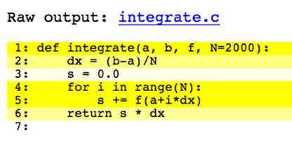
Figure 9-1. Annotated integrate without static typing
Except for line 3, all lines are a deep shade of yellow.[17] Clicking on line 2 expands it, as shown in Figure 9-2. It is clear why this line is colored yellow; there are calls to PyNumber_Subtract and __Pyx_PyNumber_Divide as well as error handling and reference counting routines.
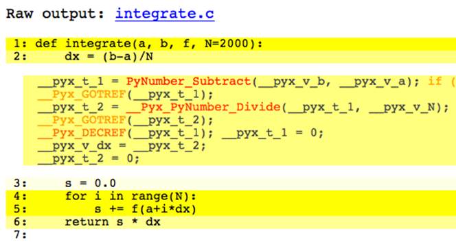
Figure 9-2. Expanded line in annotated integrate
Of particular interest is the for loop, which we expand in Figure 9-3.

Figure 9-3. Expanded annotated for loop
Without typing information, this one line of Python expands into nearly 40 lines of C code! The loop body (line 5) is similar.
Let’s add some simple static type declarations:
def integrate(double a, double b, f, int N=2000):
cdef:
int i
double dx = (b-a)/N
double s = 0.0
for i inrange(N):
s += f(a+i*dx)
return s * dx
After regenerating our annotated source file, we see in Figure 9-4 a significant difference in the code highlighting.
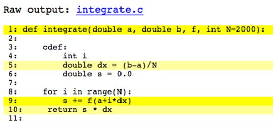
Figure 9-4. Annotated integrate with static typing
The for loop on line 8, expanded in Figure 9-5, now has no highlighting and translates to much more efficient code.
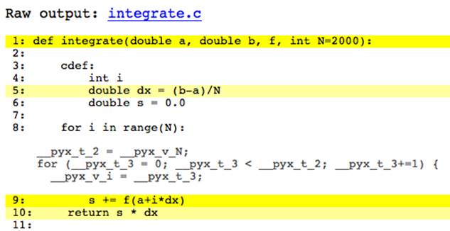
Figure 9-5. Expanded annotated for loop with static typing
Also noteworthy is the loop body, which remains highlighted. A moment’s thought reveals why: func is a dynamic Python object that we are calling in each loop iteration. We can see what the C code has to do to call a general Python object by clicking on line 9. Even though we statically typed a, i, dx, and s, we must convert the func argument to a Python object (PyFloat_FromDouble), create an argument tuple with our Python float (PyTuple_New and PyTuple_SET_ITEM), call func with this argument tuple (__Pyx_PyObject_Call), get the resulting Python object, and add it to s in place (PyNumber_InPlaceAdd). All the while, we need to do proper reference counting and error checking.
The line is yellow because the annotation heuristic picks up all the Python/C API calls and highlights accordingly. It makes it easy to see that our loop body is where we should focus our efforts to improve this function’s performance. We could, for example, make func an instance of an extension type with a call cpdef method, and inside our for loop, we could call func.call instead. This would allow us to implement compiled versions of our callback function in Cython while providing a way to subclass them in Python.
Often the first and last lines of a function are highlighted a deep shade of yellow even when all operations are C-level and should be fast. This is because the function setup and teardown logic in a def or cpdef function is grouped together during annotation; this often involves several calls into the C API and leads to the highlighting we see here. This serves as a visual indicator of Python’s function call overhead. A cdef function does not have this overhead and is not highlighted provided no Python objects are involved.
To see this, let’s write a cdef version of integrate called c_integrate. We type func as a C function pointer and turn on the cdivision compiler directive while we’re at it:[18]
cimport cython
@cython.cdivision(True)
cdef double c_integrate(double a, double b, double (*f)(double), int N=2000):
cdef:
int i
double dx = (b-a)/N
double s = 0.0
for i inrange(N):
s += f(a+i*dx)
return s * dx
The annotation for c_integrate (Figure 9-6) is encouraging—the entire function has no highlighting, indicating no C API calls were generated.
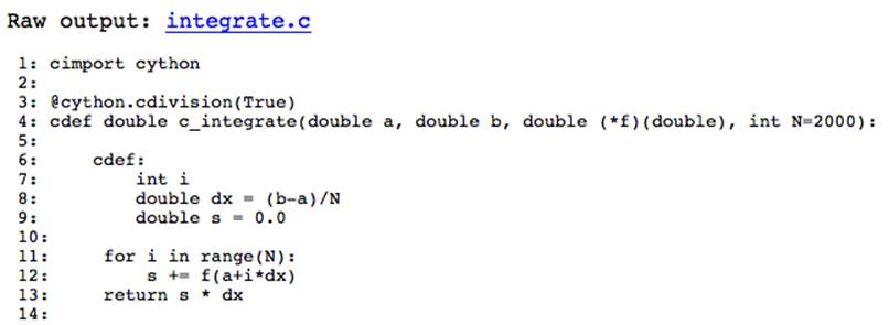
Figure 9-6. Annotated integrate without C API calls
This comes with a convenience tradeoff, of course: we lose the ability to call c_integrate from Python, so we have to create other entry points to do so. We can use c_integrate from other Cython code, of course.
Code annotations are a powerful feature to help focus efforts on possible performance bottlenecks. It is up to us to use annotations effectively. If a line of code makes many C API calls but is itself run only once, its overhead is not an important factor. On the other hand, if the code annotation indicates that a line in an inner for loop makes many C API calls, then it is likely worth the effort to improve its performance.
Keep in mind that Cython’s annotation feature provides static, compile-time performance data and uses simple heuristics to suggest which lines of code need attention. Using it in conjunction with Cython’s runtime profiling tools makes for a powerful combination.
Summary
The cardinal rule of code optimization is measure, don’t guess. Using annotations and runtime profiling together, we can let Cython tell us what code needs attention rather than guessing ourselves. Runtime profiling, which should always be the first tool we use to acquire quantitative data, tells us what routines to focus on. Code annotations can then help us determine why specific lines are slow, and can help us remove C API calls from the generated source. We split profiling and annotations into separate sections in this chapter, but in practice, their usage is often finely interleaved.
[16] To follow along with the examples in this chapter, please see https://github.com/cythonbook.
[17] In this book’s print version or on a black-and-white ereader, all figures are rendered grayscale. Please try the examples in this chapter to see the result.
[18] In this example, because no division is taking place inside the for loop, using the cdivision directive has essentially no effect on performance. We use it here to show how it removes all C API calls from the dx initialization. We could remove the cdivision directive without affecting performance.
All materials on the site are licensed Creative Commons Attribution-Sharealike 3.0 Unported CC BY-SA 3.0 & GNU Free Documentation License (GFDL)
If you are the copyright holder of any material contained on our site and intend to remove it, please contact our site administrator for approval.
© 2016-2026 All site design rights belong to S.Y.A.