Functional Python Programming (2015)
Chapter 4. Working with Collections
Python offers a number of functions that process whole collections. They can be applied to sequences (lists or tuples), sets, mappings, and iterable results of generator expressions. We'll look at some of Python's collection-processing functions from a functional programming viewpoint.
We'll start out by looking at iterables and some simple functions that work with iterables. We'll look at some additional design patterns to handle iterables and sequences with recursion as well as explicit for loops. We'll look at how we can apply a scalar() function to a collection of data with a generator expression.
In this chapter, we'll show examples of how to use the following functions to work with collections:
· any() and all()
· len() and sum() and some higher-order statistical processing related to these functions
· zip() and some related techniques to structure and flatten lists of data
· reversed()
· enumerate()
The first four functions can all be called reductions; they reduce a collection to a single value. The other three functions (zip(), reversed(), and enumerate()) are mappings; they produce a new collection from an existing collection(s). In the next chapter, we'll look at some mapping() and reduction() functions that use an additional function as an argument to customize their processing.
In this chapter, we'll start out by looking at ways to process data using generator expressions. Then, we'll apply different kinds of collection-level functions to show how they can simplify the syntax of iterative processing. We'll also look at some different ways of restructuring data.
In the next chapter, we'll focus on using higher-order collection functions to do similar kinds of processing.
An overview of function varieties
We need to distinguish between two broad species of functions, as follows:
· Scalar functions apply to individual values and compute an individual result. Functions such as abs(), pow(), and the entire math module are examples of scalar functions.
· Collection() functions work with iterable collections.
We can further subdivide the collection functions into three subspecies:
· Reduction: This uses a function that is used to fold values in the collection together, resulting in a single final value. We can call this an aggregate function, as it produces a single aggregate value for an input collection.
· Mapping: This applies a function to all items of a collection; the result is a collection of the same size.
· Filter: This applies a function to all items of a collection that rejects some items and passes others. The result is a subset of the input. A filter might do nothing, which means that the output matches the input; this is an improper subset, but it still fits the broader definition of subset.
We'll use this conceptual framework to characterize ways in which we use the built-in collection functions.
Working with iterables
As we noted in the previous chapters, we'll often use Python's for loop to work with collections. When working with materialized collections such as tuples, lists, maps, and sets, the for loop involves an explicit management of state. While this strays from purely functional programming, it reflects a necessary optimization for Python. If we assure that state management is localized to an iterator object that's created as part of the for statement evaluation, we can leverage this feature without straying too far from pure, functional programming. For example, if we use the for loop variable outside the indented body of loop, we've strayed too far from purely functional programming.
We'll return to this in Chapter 6, Recursion and Reduction. It's an important topic, and we'll just scratch the surface here with a quick example of working with generators.
One common application of for loop iterable processing is the unwrap(process(wrap(iterable))) design pattern. A wrap() function will first transform each item of an iterable into a two tuples with a derived sort key or other value and then the original immutable item. We can then process these two tuples based on the wrapped value. Finally, we'll use an unwrap() function to discard the value used to wrap, which recovers the original item.
This happens so often in a functional context that we have two functions that are used heavily for this; they are as follows:
fst = lambda x: x[0]
snd = lambda x: x[1]
These two functions pick the first and second values from a tuple, and both are handy for the process() and unwrap() functions.
Another common pattern is wrap(wrap(wrap())). In this case, we're starting with simple tuples and then wrapping them with additional results to build up larger and more complex tuples. A common variation on this theme is extend(extend(extend())) where the additional values build new, more complex namedtuple instances without actually wrapping the original tuples. We can summarize both of these as the Accretion design pattern.
We'll apply the Accretion design to work with a simple sequence of latitude and longitude values. The first step will convert the simple points (lat, lon) on a path into pairs of legs (begin, end). Each pair in the result will be ((lat, lon), (lat, lon)).
In the next sections, we'll show how to create a generator function that will iterate over the content of a file. This iterable will contain the raw input data that we will process.
Once we have the data, later sections will show how to decorate each leg with the haversine distance along the leg. The final result of the wrap(wrap(iterable()))) processing will be a sequence of three tuples: ((lat, lon), (lat, lon), distance). We can then analyze the results for the longest, shortest distance, bounding rectangle, and other summaries of the data.
Parsing an XML file
We'll start by parsing an XML (short for Extensible Markup Language) file to get the raw latitude and longitude pairs. This will show how we can encapsulate some not-quite functional features of Python to create an iterable sequence of values. We'll make use of the xml.etree module. After parsing, the resulting ElementTree object has a findall() method that will iterate through the available values.
We'll be looking for constructs such as the following code snippet:
<Placemark><Point>
<coordinates>-76.33029518659048,37.54901619777347,0</coordinates>
</Point></Placemark>
The file will have a number of <Placemark> tags, each of which has a point and coordinate structure within it. This is typical of Keyhole Markup Language (KML) files that contain geographic information.
Parsing an XML file can be approached at two levels of abstraction. At the lower level, we need to locate the various tags, attribute values, and content within the XML file. At a higher level, we want to make useful objects out of the text and attribute values.
The lower-level processing can be approached in the following way:
import xml.etree.ElementTree as XML
def row_iter_kml(file_obj):
ns_map= {
"ns0": "http://www.opengis.net/kml/2.2",
"ns1": "http://www.google.com/kml/ext/2.2"}
doc= XML.parse(file_obj)
return (comma_split(coordinates.text)
for coordinates in doc.findall("./ns0:Document/ns0:Folder/ns0:Placemark/ns0:Point/ns0:coordinates", ns_map))
This function requires a file that was already opened, usually via a with statement. However, it can also be any of the file-like objects that the XML parser can handle. The function includes a simple static dict object, ns_map, that provides the namespace mapping information for the XML tags we'll be searching. This dictionary will be used by the XML ElementTree.findall() method.
The essence of the parsing is a generator function that uses the sequence of tags located by doc.findall(). This sequence of tags is then processed by a comma_split() function to tease the text value into its comma-separated components.
The comma_split() function is the functional version of the split() method of a string, which is as follows:
def comma_split(text):
return text.split(",")
We've used the functional wrapper to emphasize a slightly more uniform syntax.
The result of this function is an iterable sequence of rows of data. Each row will be a tuple composed of three strings: latitude, longitude, and altitude of a waypoint along this path. This isn't directly useful yet. We'll need to do some more processing to get latitudeand longitude as well as converting these two numbers into useful floating-point values.
This idea of an iterable sequence of tuples as results of lower-level parsing allows us to process some kinds of data files in a simple and uniform way. In Chapter 3, Functions, Iterators, and Generators, we looked at how Comma Separated Values (CSV) files are easily handled as rows of tuples. In Chapter 6, Recursions and Reductions, we'll revisit the parsing idea to compare these various examples.
The output from the preceding function looks like the following code snippet:
[['-76.33029518659048', '37.54901619777347', '0'], ['-76.27383399999999', '37.840832', '0'], ['-76.459503', '38.331501', '0'], and so on ['-76.47350299999999', '38.976334', '0']]
Each row is the source text of the <ns0:coordinates> tag split using , that's part of the text content. The values are the East-West longitude, North-South latitude, and altitude. We'll apply some additional functions to the output of this function to create a usable set of data.
Parsing a file at a higher level
Once we've parsed the low-level syntax, we can restructure the raw data into something usable in our Python program. This kind of structuring applies to XML, JavaScript Object Notation (JSON), CSV, and any of the wide variety of physical formats in which data is serialized.
We'll aim to write a small suite of generator functions that transforms the parsed data into a form our application can use. The generator functions include some simple transformations on the text that's found by the row_iter_kml() function, which are as follows:
· Discarding altitude, or perhaps keeping only latitude and longitude
· Changing the order from (longitude, latitude) to (latitude, longitude)
We can make these two transformations have more syntactic uniformity by defining a utility function as follows:
def pick_lat_lon(lon, lat, alt):
return lat, lon
We can use this function as follows:
def lat_lon_kml(row_iter):
return (pick_lat_lon(*row) for row in row_iter)
This function will apply the pick_lat_lon() function to each row. We've used *row to assign each element of the row three tuple to separate parameters of the pick_lat_lon() function. The function can then extract and reorder the two relevant values from each three tuple.
It's important to note that a good functional design allows us to freely replace any function with its equivalent, which makes refactoring quite simple. We've tried to achieve this goal when we provide alternative implementations of the various functions. In principle, a clever functional language compiler might do some replacements as part of an optimization pass.
We'll use the following kind of processing to parse the file and build a structure we can use, such as the following code snippet:
with urllib.request.urlopen("file:./Winter%202012-2013.kml") as source:
v1= tuple(lat_lon_kml(row_iter_kml(source)))
print(v1)
We've used the urllib command to open a source. In this case, it's a local file. However, we can also open a KML file on a remote server. Our objective with using this kind of file opening is to assure that our processing is uniform no matter what the source of the data is.
We've shown the two functions that do low-level parsing of the KML source. The row_iter_kml(source) expression produces a sequence of text columns. The lat_lon_kml() function will extract and reorder the latitude and longitude values. This creates an intermediate result that sets the stage for further processing. The subsequent processing is independent of the original format.
When we run this, we see results like the following:
(('37.54901619777347', '-76.33029518659048'), ('37.840832', '-76.27383399999999'), ('38.331501', '-76.459503'), ('38.330166', '-76.458504'), ('38.976334', '-76.47350299999999'))
We've extracted just the latitude and longitude values from a complex XML file using an almost purely functional approach. As the result is an iterable, we can continue to use functional programming techniques to process each point that we retrieve from the file.
We've explicitly separated low-level XML parsing from higher-level reorganization of the data. The XML parsing produced a generic tuple of string structure. This is compatible with the output from the CSV parser. When working with SQL databases, we'll have a similar iterable of tuple structures. This allows us to write code for higher-level processing that can work with data from a variety of sources.
We'll show a series of transformations to rearrange this data from a collection of strings to a collection of waypoints along a route. This will involve a number of transformations. We'll need to restructure the data as well as convert from strings to floating-pointvalues. We'll also look at a few ways to simplify and clarify the subsequent processing steps. We'll use this data set in later chapters because it's reasonably complex.
Pairing up items from a sequence
A common restructuring requirement is to make start-stop pairs out of points in a sequence. Given a sequence, ![]() , we want to create a paired sequence
, we want to create a paired sequence ![]() . When doing time-series analysis, we might be combining more widely separated values. In this example, it's adjacent values.
. When doing time-series analysis, we might be combining more widely separated values. In this example, it's adjacent values.
A paired sequence will allow us to use each pair to compute distances from point to point using a trivial application of a haversine function. This technique is also used to convert a path of points into a series of line segments in a graphics application.
Why pair up items? Why not do something like this?
begin= next(iterable)
for end in iterable:
compute_something(begin, end)
begin = end
This, clearly, will process each leg of the data as a begin-end pair. However, the processing function and the loop that restructures the data are tightly bound, making reuse more complex than necessary. The algorithm for pairing is hard to test in isolation because it's bound to the compute_something() function.
This combined function also limits our ability to reconfigure the application. There's no easy way to inject an alternative implementation of the compute_something() function. Additionally, we've got a piece of explicit state, the begin variable, which makes life potentially complex. If we try to add features to the body of loop, we can easily fail to set the begin variable correctly if a point is dropped from consideration. A filter() function introduces an if statement that can lead to an error in updating the begin variable.
We achieve better reuse by separating this simple pairing function. This, in the long run, is one of our goals. If we build up a library of helpful primitives such as this pairing function, we can tackle problems more quickly and confidently.
There are many ways to pair up the points along the route to create start and stop information for each leg. We'll look at a few here and then revisit this in Chapter 5, Higher-order Functions and again in Chapter 8, The Itertools Module.
Creating pairs can be done in a purely functional way using a recursion. The following is one version of a function to pair up the points along a route:
def pairs(iterable):
def pair_from( head, iterable_tail ):
nxt= next(iterable_tail)
yield head, nxt
yield from pair_from( nxt, iterable_tail )
try:
return pair_from( next(iterable), iterable )
except StopIteration:
return
The essential function is the internal pair_from() function. This works with the item at the head of an iterable plus the iterable itself. It yields the first pair, pops the next item from the iterable, and then invokes itself recursively to yield any additional pairs.
We've invoked this function from the pairs() function. The pairs() function ensures that the initialization is handled properly and the terminating exception is silenced properly.
Note
Python iterable recursion involves a for loop to properly consume and yield the results from the recursion. If we try to use a simpler-looking return pair_from(nxt, iterable_tail) method, we'll see that it does not properly consume the iterable and yield all of the values.
Recursion in a generator function requires yield from a statement to consume the resulting iterable. For this, use yield from recursive_iter(args).
Something like return recursive_iter(args) will return only a generator object; it doesn't evaluate the function to return the generated values.
Our strategy for performing tail-call optimization is to replace the recursion with a generator expression. We can clearly optimize this recursion into a simple for loop. The following is another version of a function to pair up the points along a route:
def legs(lat_lon_iter):
begin= next(lat_lon_iter)
for end in lat_lon_iter:
yield begin, end
begin= end
The version is quite fast and free from stack limits. It's independent of any particular type of sequence, as it will pair up anything emitted by a sequence generator. As there's no processing function inside loop, we can reuse the legs() function as needed.
We can think of this function as one that yields the following kind of sequence of pairs:
list[0:1], list[1:2], list[2:3], ..., list[-2:]
Another view of this function is as follows:
zip(list, list[1:])
While informative, these other two formulations only work for sequence objects. The legs() and pairs() functions work for any iterable, including sequence objects.
Using the iter() function explicitly
The purely functional viewpoint is that all of our iterables can be processed with recursive functions, where the state is merely the recursive call stack. Pragmatically, Python iterables will often involve evaluation of other for loops. There are two common situations: collections and iterables. When working with a collection, an iterator object is created by the for statement. When working with a generator function, the generator function is the iterator and maintains its own internal state. Often, these are equivalent from a Python programming perspective. In rare cases, generally those situations where we have to use an explicit next() function, the two won't be precisely equivalent.
Our legs() function shown previously has an explicit next() function call to get the first value from the iterable. This works wonderfully well with generator functions, expressions, and other iterables. It doesn't work with sequence objects such as tuples or lists.
The following are three examples to clarify the use of the next() and iter() functions:
>>> list(legs(x for x in range(3)))
[(0, 1), (1, 2)]
>>> list(legs([0,1,2]))
Traceback (most recent call last):
File "<stdin>", line 1, in <module>
File "<stdin>", line 2, in legs
TypeError: 'list' object is not an iterator
>>> list(legs( iter([0,1,2])))
[(0, 1), (1, 2)]
In the first case, we applied the legs() function to an iterable. In this case, the iterable was a generator expression. This is the expected behavior based on our previous examples in this chapter. The items are properly paired up to create two legs from three waypoints.
In the second case, we tried to apply the legs() function to a sequence. This resulted in an error. While a list object and an iterable are equivalent when used in a for statement, they aren't equivalent everywhere. A sequence isn't an iterator; it doesn't implement the next() function. The for statement handles this gracefully, however, by creating an iterator from a sequence automatically.
To make the second case work, we need to explicitly create an iterator from a list object. This permits the legs() function to get the first item from the iterator over the list items.
Extending a simple loop
We have two kinds of extensions we might factor into a simple loop. We'll look first at a filter extension. In this case, we might be rejecting values from further consideration. They might be data outliers, or perhaps source data that's improperly formatted. Then, we'll look at mapping source data by performing a simple transformation to create new objects from the original objects. In our case, we'll be transforming strings to floating-point numbers. The idea of extending a simple loop with a mapping, however, applies to situations. We'll look at refactoring the above pairs() function. What if we need to adjust the sequence of points to discard a value? This will introduce a filter extension that rejects some data values.
As the loop we're designing simply returns pairs without performing any additional application-related processing, the complexity is minimal. Simplicity means we're somewhat less likely to confuse the processing state.
Adding a filter extension to this design might look something like the following code snippet:
def legs_filter(lat_lon_iter):
begin= next(lat_lon_iter)
for end in lat_lon_iter:
if #some rule for rejecting:
continue
yield begin, end
begin= end
We have plugged in a processing rule to reject certain values. As the loop remains succinct and expressive, we are confident that the processing will be done properly. Also, we can easily write a test for this function, as the results work for any iterable, irrespective of the long-term destination of the pairs.
The next refactoring will introduce additional mapping to a loop. Adding mappings is common when a design is evolving. In our case, we have a sequence of string values. We need to convert these to floating-point values for later use. This is a relatively simple mapping that shows the design pattern.
The following is one way to handle this data mapping, through a generator expression that wraps a generator function:
print(tuple(legs((float(lat), float(lon)) for lat,lon in lat_lon_kml())))
We've applied the legs() function to a generator expression that creates float values from the output of the lat_lon_kml() function. We can read this in the opposite order as well. The lat_lon_kml() function's output is transformed into a pair of float values, which is then transformed into a sequence of legs.
This is starting to get complex. We've got a large number of nested functions here. We're applying float(), legs(), and tuple() to a data generator. One common refactoring of complex expressions is to separate the generator expression from any materialized collection. We can do the following to simplify the expression:
flt= ((float(lat), float(lon)) for lat,lon in lat_lon_kml())
print(tuple(legs(flt)))
We've assigned the generator function to a variable named flt. This variable isn't a collection object; we're not using a list comprehension to create an object. We've merely assigned the generator expression to a variable name. We've then used the flt variable in another expression.
The evaluation of the tuple() method actually leads to a proper object being built so that we can print the output. The flt variable's objects are created only as needed.
There are other refactoring's we might like to do. In general, the source of the data is something we often want to change. In our example, the lat_lon_kml() function is tightly bound in the rest of the expression. This makes reuse difficult when we have a different data source.
In the case where the float() operation is something we'd like to parameterize so that we can reuse it, we can define a function around the generator expression. We'll extract some of the processing into a separate function merely to group the operations. In our case, the string-pair to float-pair is unique to a particular source data. We can rewrite a complex float-from-string expression into a simpler function such as follows:
def float_from_pair( lat_lon_iter ):
return ((float(lat), float(lon)) for lat,lon in lat_lon_iter)
The float_from_pair() function applies the float() function to the first and second values of each item in the iterable, yielding a two tuple of floats created from an input value. We've relied on Python's for statement to decompose the two tuple.
We can use this function in the following context:
legs( float_from_pair(lat_lon_kml()))
We're going to create legs that are built from float values that come from a KML file. It's fairly easy to visualize the processing, as each stage in the process is a simple prefix function.
When parsing, we often have sequences of string values. For numeric applications, we'll need to convert strings to float, int, or Decimal values. This often involves inserting a function such as the float_from_pair() function into a sequence of expressions that clean up the source data.
Our previous output was all strings; it looked like the following code snippet:
(('37.54901619777347', '-76.33029518659048'), ('37.840832', '-76.27383399999999'), ... ('38.976334', '-76.47350299999999'))
We'll want data like the following code snippet, where we have floats:
(((37.54901619777347, -76.33029518659048), (37.840832, -76.273834)), ((37.840832, -76.273834), … ((38.330166, -76.458504), (38.976334, -76.473503)))
We'll need to create a pipeline of simpler transformation functions. Above, we arrived at flt= ((float(lat), float(lon)) for lat,lon in lat_lon_kml()). We can exploit the substitution rule for functions and replace a complex expression such as (float(lat), float(lon)) for lat,lon in lat_lon_kml()) with a function that has the same value, in this case, float_from_pair(lat_lon_kml()). This kind of refactoring allows us to be sure that a simplification has the same effect as a more complex expression.
There are some simplifications that we'll look at in Chapter 5, Higher-order Functions. We will revisit this in Chapter 6, Recursions and Reductions to see how to apply these simplifications to the file-parsing problem.
Applying generator expressions to scalar functions
We'll look cat a more complex kind of generator expression to map data values from one kind of data to another. In this case, we'll apply a fairly complex function to individual data values created by a generator.
We'll call these non-generator functions scalar, as they work with simple scalar values. To work with collections of data, a scalar function will be embedded in a generator expression.
To continue the example started earlier, we'll provide a haversine function and then use a generator expression to apply a scalar haversine() function to a sequence of pairs from our KML file.
The haversine() function looks like following:
from math import radians, sin, cos, sqrt, asin
MI= 3959
NM= 3440
KM= 6371
def haversine( point1, point2, R=NM ):
lat_1, lon_1= point1
lat_2, lon_2= point2
Δ_lat = radians(lat_2 - lat_1)
Δ_lon = radians(lon_2 - lon_1)
lat_1 = radians(lat_1)
lat_2 = radians(lat_2)
a = sin(Δ_lat/2)**2 + cos(lat_1)*cos(lat_2)*sin(Δ_lon/2)**2
c = 2*asin(sqrt(a))
return R * c
This is a relatively simple implementation copied from the World Wide Web.
The following is how we might use our collection of functions to examine some KML data and produce a sequence of distances:
trip= ((start, end, round(haversine(start, end),4))
for start,end in legs(float_from_pair(lat_lon_kml())))
for start, end, dist in trip:
print(start, end, dist)
The essence of the processing is the generator expression assigned to the trip variable. We've assembled three tuples with a start, end, and the distance from start to end. The start and end pairs come from the legs() function. The legs() function works withfloating-point data built from the latitude-longitude pairs extracted from a KML file.
The output looks like the following command snippet:
(37.54901619777347, -76.33029518659048) (37.840832, -76.273834) 17.7246
(37.840832, -76.273834) (38.331501, -76.459503) 30.7382
(38.331501, -76.459503) (38.845501, -76.537331) 31.0756
(36.843334, -76.298668) (37.549, -76.331169) 42.3962
(37.549, -76.331169) (38.330166, -76.458504) 47.2866
(38.330166, -76.458504) (38.976334, -76.473503) 38.8019
Each individual processing step has been defined succinctly. The overview, similarly, can be expressed succinctly as a composition of functions and generator expressions.
Clearly, there are several further processing steps we might like to apply to this data. First, of course, is to use the format() method of a string to produce better-looking output.
More importantly, there are a number of aggregate values we'd like to extract from this data. We'll call these values reductions of the available data. We'd like to reduce the data to get the maximum and minimum latitude—for example, to show the extreme North and South ends of this route. We'd like to reduce the data to get the maximum distance in one leg as well as the total distance for all legs.
The problem we'll have using Python is that the output generator in the trip variable can only be used once. We can't easily perform several reductions of this detailed data. We can use itertools.tee() to work with the iterable several times. It seems wasteful, however, to read and parse the KML file for each reduction.
We can make our processing more efficient by materializing intermediate results. We'll look at this in the next section. Then, we can see how to compute multiple reductions of the available data.
Using any() and all() as reductions
The any() and all() functions provide boolean reduction capabilities. Both functions reduce a collection of values to a single True or False. The all() function assures that all values are True. The any() function assures that at least one value is True.
These functions are closely related to a universal quantifier and an existential quantifier used to express mathematical logic. We might, for example, want to assert that all elements in a given collection have some property. One formalism for this might look like following:
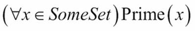
We'd read this as: for all x in SomeSet, the function ![]() is true. We've put a quantifier in front of the logical expression.
is true. We've put a quantifier in front of the logical expression.
In Python, we switch the order of the items slightly to transcribe the logic expression as follows:
all(isprime(x) for x in someset)
This will evaluate each argument value (isprime(x)) and reduce the collection of values to a single True or False.
The any() function is related to the existential quantifier. If we want to assert that no value in a collection is prime, we might have something like one of the two equivalent expressions:

The first states that it is not the case that all elements in SomeSet are prime. The second version asserts that there exists one element in SomeSet that is not prime. These two are equivalent—that is, if not all elements are prime, then one element must be non-prime.
In Python, we can switch the order of the terms and transcribe these to working code as follows:
not all(isprime(x) for x in someset)
any(not isprime(x) for x in someset)
As they're equivalent, there are two reasons for preferring one over the other: performance and clarity. The performance is nearly identical, so it boils down to clarity. Which of these states the condition the most clearly?
The all() function can be described as an and reduction of a set of values. The result is similar to folding the and operator between the given sequence of values. The any() function, similarly, can be described as an or reduction. We'll return to this kind of general-purpose reduce when we look at the reduce() function in Chapter 10, The Functools Module.
We also need to look at the degenerate case of these functions. What if the sequence has 0 elements? What are the values of all(()) or all([])?
If we ask, "Are all elements in an empty set prime?", then what's the answer? As there are no elements, the question is a bit difficult to answer.
If we ask "Are all elements in an empty set prime and all elements in SomeSet prime?", we have a hint as to how we have to proceed. We're performing an and reduction of an empty set and an and reduction of SomeSet.

It turns out that the and operator can be distributed freely. We can rewrite this to a union of the two sets, which is then evaluated for being prime:
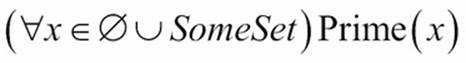
Clearly, ![]() . If we union an empty set, we get the original set. The empty set can be called the union identify element. This parallels the way 0 is the additive identity element:
. If we union an empty set, we get the original set. The empty set can be called the union identify element. This parallels the way 0 is the additive identity element: ![]() .
.
Similarly, any(()) must be the or identity element, which is False. If we think of the multiplicative identify element, 1, where ![]() , then all(()) must be True.
, then all(()) must be True.
We can demonstrate that Python follows these rules:
>>> all(())
True
>>> any(())
False
Python gives us some very nice tools to perform processing that involves logic. We have the built-in and, or, and not operators. However, we also have these collection-oriented any() and all() functions.
Using len() and sum()
The len() and sum() functions provide two simple reductions: a count of the elements and the sum of the elements in a sequence. These two functions are mathematically similar, but their Python implementation is quite different.
Mathematically, we can observe this cool parallelism. The len() function returns the sum of 1's for each value in a collection, X:![]() .
.
The sum() function returns the sum of x for each value in a collection, X:![]() .
.
The sum() function works for any iterable. The len() function doesn't apply to iterables; it only applies to sequences. This little asymmetry in the implementation of these functions is a little awkward around the edges of statistical algorithms.
For empty sequences, both of these functions return a proper additive identity element of 0.
>>> sum(())
0
Of course, sum(()) returns an integer 0. When other numeric types are used, the integer 0 will be coerced to the proper type for the available data.
Using sums and counts for statistics
The definitions of the arithmetic mean have an appealingly trivial definition based on sum() and len(), which is as follows:
def mean( iterable ):
return sum(iterable)/len(iterable)
While elegant, this doesn't actually work for iterables. This definition only works for sequences.
Indeed, we have a hard time performing a simple computation of mean or standard deviation based on iterables. In Python, we must either materialize a sequence object, or resort to somewhat more complex operations.
We have a fairly elegant expression of mean and standard deviation in the following definitions:
import math
s0= len(data) # sum(1 for x in data) # x**0
s1= sum(data) # sum(x for x in data) # x**1
s2= sum(x*x for x in data)
mean= s1/s0
stdev= math.sqrt(s2/s0 - (s1/s0)**2)
These three sums, s0, s1, and s2, have a tidy, parallel structure. We can easily compute the mean from two of the sums. The standard deviation is a bit more complex, but it's still based on the three sums.
This kind of pleasant symmetry also works for more complex statistical functions such as correlation and even least-squares linear regression.
The moment of correlation between two sets of samples can be computed from their standardized value. The following is a function to compute the standardized value:
def z( x, μ_x, σ_x ):
return (x-μ_x)/σ_x
The calculation is simply to subtract the mean, μ_x, from each sample, x, and divide by the standard deviation, σ_x. This gives as a value measured in units of sigma, σ. A value ±1 σ is expected about two-thirds of the time. Larger values should be less common. A value outside ±3 σ should happen less than 1 percent of the time.
We can use this scalar function as follows:
>>> d = [2, 4, 4, 4, 5, 5, 7, 9]
>>> list(z(x, mean(d), stdev(d)) for x in d)
[-1.5, -0.5, -0.5, -0.5, 0.0, 0.0, 1.0, 2.0]
We've materialized list that consists of normalized scores based on some raw data in the variable, d. We used a generator expression to apply the scalar function, z(), to the sequence object.
The mean() and stdev() functions are simply based on the examples shown above:
def mean(x):
return s1(x)/s0(x)
def stdev(x):
return math.sqrt(s2(x)/s0(x) - (s1(x)/s0(x))**2)
The three sum functions, similarly, are based on the examples above:
def s0(data):
return sum(1 for x in data) # or len(data)
def s1(data):
return sum(x for x in data) # or sum(data)
def s2(data):
return sum(x*x for x in data)
While this is very expressive and succinct, it's a little frustrating because we can't simply use an iterable here. We're computing a mean, which requires a sum of the iterable, plus a count. We're also computing a standard deviation that requires two sums and a count from the iterable. For this kind of statistical processing, we must materialize a sequence object so that we can examine the data multiple times.
The following is how we can compute the correlation between two sets of samples:
def corr( sample1, sample2 ):
μ_1, σ_1 = mean(sample1), stdev(sample1)
μ_2, σ_2 = mean(sample2), stdev(sample2)
z_1 = (z(x, μ_1, σ_1) for x in sample1)
z_2 = (z(x, μ_2, σ_2) for x in sample2)
r = sum(zx1*zx2 for zx1, zx2 in zip(z_1, z_2) )/s0(sample1)
return r
This correlation function gathers basic statistical summaries of the two sets of samples: the mean and standard deviation. Given these summaries, we defined two generator functions that will create normalized values for each set of samples. We can then use thezip() function (see the next example) to pair up items from the two sequences of normalized values and compute the product of those two normalized values. The average of the product of the normalized scores is the correlation.
The following is an example of gathering the correlation between two sets of samples:
>>> xi= [1.47, 1.50, 1.52, 1.55, 1.57, 1.60, 1.63, 1.65,... 1.68, 1.70, 1.73, 1.75, 1.78, 1.80, 1.83,] # Height (m)
>>> yi= [52.21, 53.12, 54.48, 55.84, 57.20, 58.57, 59.93, 61.29,... 63.11, 64.47, 66.28, 68.10, 69.92, 72.19, 74.46,] # ... Mass (kg)
>>> round(corr( xi, yi ), 5)
0.99458
We've shown two sequences of data points, xi and yi. The correlation is over .99, which shows a very strong relationship between the two sequences.
This shows one of the strengths of functional programming. We've created a handy statistical module using a half-dozen functions with definitions that are single expressions. The counterexample is the corr() function that can be reduced to a single very long expression. Each internal variable in this function is used just once; a local variable can be replaced with a copy-and-paste of the expression that created it. This shows us that the corr() function has a functional design even though it's written out in six separate lines of Python.
Using zip() to structure and flatten sequences
The zip() function interleaves values from several iterators or sequences. It will create n tuples from the values in each of the n input iterables or sequences. We used it in the previous section to interleave data points from two sets of samples, creating two tuples.
Note
The zip() function is a generator. It does not materialize a resulting collection.
The following is an example that shows what the zip() function does:
>>> xi= [1.47, 1.50, 1.52, 1.55, 1.57, 1.60, 1.63, 1.65,... 1.68, 1.70, 1.73, 1.75, 1.78, 1.80, 1.83,]
>>> yi= [52.21, 53.12, 54.48, 55.84, 57.20, 58.57, 59.93, 61.29,... 63.11, 64.47, 66.28, 68.10, 69.92, 72.19, 74.46,]
>>> zip( xi, yi )
<zip object at 0x101d62ab8>
>>> list(zip( xi, yi ))
[(1.47, 52.21), (1.5, 53.12), (1.52, 54.48), (1.55, 55.84), (1.57, 57.2), (1.6, 58.57), (1.63, 59.93), (1.65, 61.29), (1.68, 63.11), (1.7, 64.47), (1.73, 66.28), (1.75, 68.1), (1.78, 69.92), (1.8, 72.19), (1.83, 74.46)]
There are a number of edge cases for the zip() function. We must ask the following questions about its 'margin-left:18.0pt;text-indent:-18.0pt;line-height: normal'>· What happens where then are no arguments at all?
· What happens where there's only one argument?
· What happens when the sequences are different lengths?
For reductions (any(), all(), len(), sum()), we want an identity element from reducing an empty sequence.
Clearly, each of these edge cases must produce some kind of iterable output. Here are some examples to clarify the behaviors. First, the empty argument list:
>>> zip()
<zip object at 0x101d62ab8>
>>> list(_)
[]
We can see that the zip() function with no arguments is a generator function, but there won't be any items. This fits the requirement that the output is iterable.
Next, we'll try a single iterable:
>>> zip( (1,2,3) )
<zip object at 0x101d62ab8>
>>> list(_)
[(1,), (2,), (3,)]
In this case, the zip() function emitted one tuple from each input value. This too makes considerable sense.
Finally, we'll look at the different-length list approach used by the zip() function:
>>> list(zip((1, 2, 3), ('a', 'b')))
[(1, 'a'), (2, 'b')]
This result is debatable. Why truncate? Why not pad the shorter list with None values? This alternate definition of zip() function is available in the itertools module as the zip_longest() function. We'll look at this in Chapter 8, The Itertools Module.
Unzipping a zipped sequence
zip() mapping can be inverted. We'll look at several ways to unzip a collection of tuples.
Note
We can't fully unzip an iterable of tuples, since we might want to make multiple passes over the data. Depending on our needs, we might need to materialize the iterable to extract multiple values.
The first way is something we've seen many times; we can use a generator function to unzip a sequence of tuples. For example, assume that the following pairs are a sequence object with two tuples:
p0= (x[0] for x in pairs)
p1= (x[1] for x in pairs)
This will create two sequences. The p0 sequence has the first element of each two tuple; the p1 sequence has the second element of each two tuple.
Under some circumstances, we can use the multiple ssignment of a for loop to decompose the tuples. The following is an example that computes the sum of products:
sum(p0*p1 for for p0, p1 in pairs)
We used the for statement to decompose each two tuple into p0 and p1.
Flattening sequences
Sometimes, we'll have zipped data that needs to be flattened. For example, our input might be a file that looks like this:
2 3 5 7 11 13 17 19 23 29
31 37 41 43 47 53 59 61 67 71
...
We can easily use ((line.split() for line in file) to create a sequence of ten tuples.
We might heave data in blocks that looks as follows:
blocked = [['2', '3', '5', '7', '11', '13', '17', '19', '23', '29'], ['31', '37', '41', '43', '47', '53', '59', '61', '67', '71'],...
This isn't really what we want, though. We want to get the numbers into a single, flat sequence. Each item in the input is a ten tuple; we'd rather not wrangle with decomposing this one item at a time.
We can use a two-level generator expression, as shown in the following code snippet, for this kind of flattening:
>>> (x for line in blocked for x in line)
<generator object <genexpr> at 0x101cead70>
>>> list(_)
['2', '3', '5', '7', '11', '13', '17', '19', '23', '29', '31', '37', '41', '43', '47', '53', '59', '61', '67', '71', … ]
The two-level generator is confusing at first. We can understand this through a simple rewrite as follows:
for line in data:
for x in line:
yield x
This transformation shows us how the generator expression works. The first for clause (for line in data) steps through each ten tuple in the data. The second for clause (for x in line) steps through each item in the first for clause.
This expression flattens a sequence-of-sequence structure into a single sequence.
Structuring flat sequences
Sometimes, we'll have raw data that is a flat list of values that we'd like to bunch up into subgroups. This is a bit more complex. We can use the itertools module's groupby() function to implement this. This will have to wait until Chapter 8, The Iterools Module.
Let's say we have a simple flat list as follows:
flat= ['2', '3', '5', '7', '11', '13', '17', '19', '23', '29', '31', '37', '41', '43', '47', '53', '59', '61', '67', '71', ... ]
We can write nested generator functions to build a sequence-of-sequence structure from flat data. In order to do this, we'll need a single iterator that we can use multiple times. The expression looks like the following code snippet:
>>> flat_iter=iter(flat)
>>> (tuple(next(flat_iter) for i in range(5)) for row in range(len(flat)//5))
<generator object <genexpr> at 0x101cead70>
>>> list(_)
[('2', '3', '5', '7', '11'), ('13', '17', '19', '23', '29'), ('31', '37', '41', '43', '47'), ('53', '59', '61', '67', '71'), ('73', '79', '83', '89', '97'), ('101', '103', '107', '109', '113'), ('127', '131', '137', '139', '149'), ('151', '157', '163', '167', '173'), ('179', '181', '191', '193', '197'), ('199', '211', '223', '227', '229')]
First, we created an iterator that exists outside either of the two loops that we'll use to create our sequence-of-sequences. The generator expression uses tuple(next(flat_iter) for i in range(5)) to create five tuples from the iterable values in the flat_iter variable. This expression is nested inside another generator that repeats the inner loop the proper number of times to create the required sequence of values.
This works only when the flat list is divided evenly. If the last row has partial elements, we'll need to process them separately.
We can use this kind of function to group data into same-sized tuples, with an odd sized tuple at the end using the following definitions:
def group_by_seq(n, sequence):
flat_iter=iter(sequence)
full_sized_items = list( tuple(next(flat_iter)
for i in range(n))
for row in range(len(sequence)//n))
trailer = tuple(flat_iter)
if trailer:
return full_sized_items + [trailer]
else:
return full_sized_items
We've created an initial list where each tuple is of the size n. If there are leftovers, we'll have a trailer tuple with a non-zero length that we can append to the list of full-sized items. If the trailer tuple is of the length 0, we'll ignore it.
This isn't as delightfully simple and functional-looking as other algorithms we've looked at. We can rework this into a pleasant-enough generator function. The following code uses a while loop as part of tail-recursion optimization:
def group_by_iter( n, iterable ):
row= tuple(next(iterable) for i in range(n))
while row:
yield row
row= tuple(next(iterable) for i in range(n))
We've created a row of the required length from the input iterable. When we get to the end of the input iterable, the value of tuple(next(iterable) for i in range(n)) will be a zero-length tuple. This is the base case of a recursion, which we've written as the terminating condition for a while loop.
Structuring flat sequences—an alternative approach
Let's say we have a simple, flat list and we want to create pairs from this list. The following is the required data:
flat= ['2', '3', '5', '7', '11', '13', '17', '19', '23', '29', '31', '37', '41', '43', '47', '53', '59', '61', '67', '71',... ]
We can create pairs using list slices as follows:
zip(flat[0::2], flat[1::2])
The slice flat[0::2] is all of the even positions. The slice flat[1::2] is all of the odd positions. If we zip these together, we get a two tuple of (0), the value from the first even position, and (1), the value from the first odd position. If the number of elements is even, this will produce pairs nicely.
This has the advantage of being quite short. The functions shown in the previous section are longer ways to solve the same problem.
This approach can be generalized. We can use the *(args) approach to generate a sequence-of-sequences that must be zipped together. It looks like the following:
zip(*(flat[i::n] for i in range(n)))
This will generate n slices: flat[0::n], flat[1::n], flat[2::n], …, flat[n-1::n]. This collection of slices becomes the arguments to zip(), which then interleaves values from each slice.
Recall that zip() truncates the sequence at the shortest list. This means that, if the list is not an even multiple of the grouping factor n, (len(flat)%n != 0), which is the final slice, won't be the same length as the others and the others will all be truncated. This is rarely what we want.
If we use the itertools.zip_longest() method, then we'll see that the final tuple will be padded with enough None values to make it have a length of n. In some cases, this padding is acceptable. In other cases, the extra values are undesirable.
The list slicing approach to grouping data is another way to approach the problem of structuring a flat sequence of data into blocks. As it is a general solution, it doesn't seem to offer too many advantages over the functions in the previous section. As a solution specialized for making two tuples from a flat last, it's elegantly simple.
Using reversed() to change the order
There are times when we need a sequence reversed. Python offers us two approaches to this: the reversed() function and slices with reversed indices.
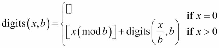
For an example, consider performing a base conversion to hexadecimal or binary. The following is a simple conversion function:
def digits(x, b):
if x == 0: return
yield x % b
for d in to_base(x//b, b):
yield d
This function uses a recursion to yield the digits from the least significant to the most significant. The value of x%b will be the least significant digits of x in the base b.
We can formalize it as following:
In many cases, we'd prefer the digits to be yielded in the reverse order. We can wrap this function with the reversed() function to swap the order of the digits:
def to_base(x, b):
return reversed(tuple(digits(x, b)))
Note
The reversed() function produces an iterable, but the argument value must be a sequence object. The function then yields the items from that object in the reverse order.
We can do a similar kind of thing also with a slice such as tuple(digits(x, b))[::-1]. The slice, however, is not an iterator. A slice is a materialized object built from another materialized object. In this case, for such small collections of values, the distinction is minor. As the reversed() function uses less memory, it might be advantageous for larger collections.
Using enumerate() to include a sequence number
Python offers the enumerate() function to apply index information to values in a sequence or iterable. It performs a specialized kind of wrap that can be used as part of an unwrap(process(wrap(data))) design pattern.
It looks like the following code snippet:
>>> xi
[1.47, 1.5, 1.52, 1.55, 1.57, 1.6, 1.63, 1.65, 1.68, 1.7, 1.73, 1.75, 1.78, 1.8, 1.83]
>>> list(enumerate(xi))
[(0, 1.47), (1, 1.5), (2, 1.52), (3, 1.55), (4, 1.57), (5, 1.6), (6, 1.63), (7, 1.65), (8, 1.68), (9, 1.7), (10, 1.73), (11, 1.75), (12, 1.78), (13, 1.8), (14, 1.83)]
The enumerate() function transformed each input item into a pair with a sequence number and the original item. It's vaguely similar to something as follows:
zip(range(len(source)), source)
An important feature of enumerate() is that the result is an iterable and it works with any iterable input.
When looking at statistical processing, for example, the enumerate() function comes in handy to transform a single sequence of values into a more proper time series by prefixing each sample with a number.
Summary
In this chapter, we saw detailed ways to use a number of built-in reductions.
We've used any() and all() to do essential logic processing. These are tidy examples of reductions using a simple operator such as or or and.
We've also looked at numeric reductions such as len() and sum(). We've applied these functions to create some higher-order statistical processing. We'll return to these reductions in Chapter 6, Recursions and Reductions.
We've also looked at some of the built-in mappings.
The zip() function merges multiple sequences. This leads us to look at using this in the context of structuring and flattening more complex data structures. As we'll see in examples in later chapters, nested data is helpful in some situations and flat data is helpful in others.
The enumerate() function maps an iterable to a sequence of two tuples. Each two tuple has (0) as the sequence number and (1) as the original item.
The reversed() function iterates over the items in a sequence object with their original order reversed. Some algorithms are more efficient at producing results in one order, but we'd like to present these results in the opposite order.
In the next chapter, we'll look at the mapping and reduction functions that use an additional function as an argument to customize their processing. Functions that accept a function as an argument are our first examples of higher-order functions. We'll also touch on functions that return functions as a result.
All materials on the site are licensed Creative Commons Attribution-Sharealike 3.0 Unported CC BY-SA 3.0 & GNU Free Documentation License (GFDL)
If you are the copyright holder of any material contained on our site and intend to remove it, please contact our site administrator for approval.
© 2016-2026 All site design rights belong to S.Y.A.