DOING MATH WITH PYTHON Use Programming to Explore Algebra, Statistics, Calculus, and More! (2015)

In this chapter, we’ll use Python to explore statistics so we can study, describe, and better understand sets of data. After looking at some basic statistical measures—the mean, median, mode, and range—we’ll move on to some more advanced measures, such as variance and standard deviation. Then, we’ll see how to calculate the correlation coefficient, which allows you to quantify the relationship between two sets of data. We’ll end the chapter by learning about scatter plots. Along the way, we’ll learn more about the Python language and standard library modules. Let’s get started with one of the most commonly used statistical measures—the mean.

NOTE

In statistics, some statistical measures are calculated slightly differently depending on whether you have data for an entire population or just a sample. To keep things simple, we’ll stick with the calculation methods for a population in this chapter.

Finding the Mean

The mean is a common and intuitive way to summarize a set of numbers. It’s what we might simply call the “average” in everyday use, although as we’ll see, there are other kinds of averages as well. Let’s take a sample set of numbers and calculate the mean.

Say there’s a school charity that’s been taking donations over a period of time spanning the last 12 days (we’ll refer to this as period A). In that time, the following 12 numbers represent the total dollar amount of donations received for each day: 100, 60, 70, 900, 100, 200, 500, 500, 503, 600, 1000, and 1200. We can calculate the mean by summing these totals and then dividing the sum by the number of days. In this case, the sum of the numbers is 5733. If we divide this number by 12 (the number of days), we get 477.75, which is the mean donation per day. This number gives us a general idea of how much money was donated on any given day.

In a moment, we’ll write a program that calculates and prints the mean for a collection of numbers. As we just saw, to calculate the mean, we’ll need to take the sum of the list of numbers and divide it by the number of items in the list. Let’s look at two Python functions that make both of these operations very easy: sum() and len().

When you use the sum() function on a list of numbers, it adds up all the numbers in the list and returns the result:

>>> shortlist = [1, 2, 3]
>>> sum(shortlist)
6

We can use the len() function to give us the length of a list:

>>> len(shortlist)
3

When we use the len() function on the list, it returns 3 because there are three items in shortlist. Now we’re ready to write a program that will calculate the mean of the list of donations.

'''
Calculating the mean
'''

def calculate_mean(numbers):
➊ s = sum(numbers)
➋ N = len(numbers)
# Calculate the mean
➌ mean = s/N

return mean

if __name__ == '__main__':
➍ donations = [100, 60, 70, 900, 100, 200, 500, 500, 503, 600, 1000, 1200]
➎ mean = calculate_mean(donations)
N = len(donations)
➏ print('Mean donation over the last {0} days is {1}'.format(N, mean))

First, we define a function, calculate_mean(), that accepts the argument numbers, which is a list of numbers. At ➊, we use the sum() function to add up the numbers in the list and create a label, s, to refer to the total. Similarly, at ➋, we use the len() function to get the length of the list and create a label, N, to refer to it. Then, as you can see at ➌, we calculate the mean by simply dividing the sum (s) by the number of members (N). At ➍, we create a list, donations, with the values of the donations listed earlier. We then call the calculate_mean() function, passing this list as an argument at ➎. Finally, we print the mean that was calculated at ➏.

When you run the program, you should see the following:

Mean donation over the last 12 days is 477.75

The calculate_mean() function will calculate the sum and length of any list, so we can reuse it to calculate the mean for other sets of numbers, too.

We calculated that the mean donation per day was 477.75. It’s worth noting that the donations during the first few days were much lower than the mean donation we calculated and that the donations during the last couple of days were much higher. The mean gives us one way to summarize the data, but it doesn’t give us a full picture. There are other statistical measurements, however, that can tell us more about the data when compared with the mean.

Finding the Median

The median of a collection of numbers is another kind of average. To find the median, we sort the numbers in ascending order. If the length of the list of numbers is odd, the number in the middle of the list is the median. If the length of the list of numbers is even, we get the median by taking the mean of the two middle numbers. Let’s find the median of the previous list of donations: 100, 60, 70, 900, 100, 200, 500, 500, 503, 600, 1000, and 1200.

After sorting from smallest to largest, the list of numbers becomes 60, 70, 100, 100, 200, 500, 500, 503, 600, 900, 1000, and 1200. We have an even number of items in the list (12), so to get the median, we need to take the mean of the two middle numbers. In this case, the middle numbers are the sixth and the seventh numbers—500 and 500—and the mean of these two numbers is (500 + 500)/2, which comes out to 500. That means the median is 500.

Now assume—just for this example—that we have another donation total for the 13th day so that the list now looks like this: 100, 60, 70, 900, 100, 200, 500, 500, 503, 600, 1000, 1200, and 800.

Once again, we have to sort the list, which becomes 60, 70, 100, 100, 200, 500, 500, 503, 600, 800, 900, 1000, and 1200. There are 13 numbers in this list (an odd number), so the median for this list is simply the middle number. In this case, that’s the seventh number, which is 500.

Before we write a program to find the median of a list of numbers, let’s think about how we could automatically calculate the middle elements of a list in either case. If the length of a list (N) is odd, the middle number is the one in position (N + 1)/2. If N is even, the two middle elements are N/2 and (N/2) + 1. For our first example in this section, N = 12, so the two middle elements were the 12/2 (sixth) and 12/2 + 1 (seventh) elements. In the second example, N = 13, so the seventh element, (N + 1)/2, was the middle element.

In order to write a function that calculates the median, we’ll also need to sort a list in ascending order. Luckily, the sort() method does just that:

>>> samplelist = [4, 1, 3]
>>> samplelist.sort()
>>> samplelist
[1, 3, 4]

Now we can write our next program, which finds the median of a list of numbers:

'''
Calculating the median
'''

def calculate_median(numbers):
➊ N = len(numbers)
➋ numbers.sort()

# Find the median
if N % 2 == 0:
# if N is even
m1 = N/2
m2 = (N/2) + 1
# Convert to integer, match position
➌ m1 = int(m1) - 1
➍ m2 = int(m2) - 1
➎ median = (numbers[m1] + numbers[m2])/2
else:
➏ m = (N+1)/2
# Convert to integer, match position
m = int(m) - 1
median = numbers[m]

return median

if __name__ == '__main__':
donations = [100, 60, 70, 900, 100, 200, 500, 500, 503, 600, 1000, 1200]

median = calculate_median(donations)
N = len(donations)
print('Median donation over the last {0} days is {1}'.format(N, median))

The overall structure of the program is similar to that of the earlier program that calculates the mean. The calculate_median() function accepts a list of numbers and returns the median. At ➊, we calculate the length of the list and create a label, N, to refer to it. Next, at ➋, we sort the list using the sort() method.

Then, we check to see whether N is even. If so, we find the middle elements, m1 and m2, which are the numbers at positions N/2 and (N/2) + 1 in the sorted list. The next two statements (➌ and ➍) adjust m1 and m2 in two ways. First, we use the int() function to convert m1 and m2 into integer form. This is because results of the division operator are always returned as floating point numbers, even when the result is equivalent to an integer. For example:

>>> 6/2
3.0

We cannot use a floating point number as an index in a list, so we use int() to convert that result to an integer. We also subtract 1 from both m1 and m2 because positions in a list begin with 0 in Python. This means that to get the sixth and seventh numbers from the list, we have to ask for the numbers at index 5 and index 6. At ➎, we calculate the median by taking the mean of the two numbers in the middle positions.

Starting at ➏, the program finds the median if there’s an odd number of items in the list, once again using int() and subtracting 1 to find the proper index. Finally, the program calculates the median for the list of donations and returns it. When you execute the program, it calculates that the median is 500:

Median donation over the last 12 days is 500.0

As you can see, the mean (477.75) and the median (500) are pretty close in this particular list, but the median is a little higher.

Finding the Mode and Creating a Frequency Table

Instead of finding the mean value or the median value of a set of numbers, what if you wanted to find the number that occurs most frequently? This number is called the mode. For example, consider the test scores of a math test (out of 10 points) in a class of 20 students: 7, 8, 9, 2, 10, 9, 9, 9, 9, 4, 5, 6, 1, 5, 6, 7, 8, 6, 1, and 10. The mode of this list would tell you which score was the most common in the class. From the list, you can see that the score of 9 occurs most frequently, so 9 is the mode for this list of numbers. There’s no symbolic formula for calculating the mode—you simply count how many times each unique number occurs and find the one that occurs the most.

To write a program to calculate the mode, we’ll need to have Python count how many times each number occurs within a list and print the one that occurs most frequently. The Counter class from the collections module, which is part of the standard library, makes this really simple for us.

Finding the Most Common Elements

Finding the most common number in a data set can be thought of as a subproblem of finding an arbitrary number of most common numbers. For instance, instead of the most common score, what if you wanted to know the five most common scores? The most_common() method of the Counterclass allows us to answer such questions easily. Let’s see an example:

>>> simplelist = [4, 2, 1, 3, 4]
>>> from collections import Counter
>>> c = Counter(simplelist)
>>> c.most_common()
[(4, 2), (1, 1), (2, 1), (3, 1)]

Here, we start off with a list of five numbers and import Counter from the collections module. Then, we create a Counter object, using c to refer to the object. We then call the most_common() method, which returns a list ordered by the most common elements.

Each member of the list is a tuple. The first element of the first tuple is the number that occurs most frequently, and the second element is the number of times it occurs. The second, third, and fourth tuples contain the other numbers along with the count of the number of times they appear. This result tells us that 4 occurs the most (twice), while the others appear only once. Note that numbers that occur an equal number of times are returned by the most_common() method in an arbitrary order.

When you call the most_common() method, you can also provide an argument telling it the number of most common elements you want it to return. For example, if we just wanted to find the most common element, we would call it with the argument 1:

>>> c.most_common(1)
[(4, 2)]

If you call the method again with 2 as an argument, you’ll see this:

>>> c.most_common(2)
[(4, 2), (1, 1)]

Now the result returned by the most_common method is a list with two tuples. The first is the most common element, followed by the second most common. Of course, in this case, there are several elements tied for most common, so the fact that the function returns 1 here (and not 2 or 3) is arbitrary, as noted earlier.

The most_common() method returns both the numbers and the number of times they occur. What if we want only the numbers and we don’t care about the number of times they occur? Here’s how we can retrieve that information:

➊ >>> mode = c.most_common(1)
>>> mode
[(4, 2)]
➋ >>> mode[0]
(4, 2)
➌ >>> mode[0][0]
4

At ➊, we use the label mode to refer to the result returned by the most_common() method. We retrieve the first (and the only) element of this list with mode[0] ➋, which gives us a tuple. Because we just want the first element of the tuple, we can retrieve that using mode[0][0] ➌. This returns 4— the most common element, or the mode.

Now that we know how the most_common() method works, we’ll apply it to solve the next two problems.

Finding the Mode

We’re ready to write a program that finds the mode for a list of numbers:

'''
Calculating the mode
'''

from collections import Counter

def calculate_mode(numbers):
➊ c = Counter(numbers)
➋ mode = c.most_common(1)
➌ return mode[0][0]

if __name__=='__main__':
scores = [7,8,9,2,10,9,9,9,9,4,5,6,1,5,6,7,8,6,1,10]
mode = calculate_mode(scores)

print('The mode of the list of numbers is: {0}'.format(mode))

The calculate_mode() function finds and returns the mode of the numbers passed to it as a parameter. To calculate the mode, we first import the class Counter from the collections module and use it to create a Counter object at ➊. Then, at ➋, we use the most_common() method, which, as we saw earlier, gives us a list that contains a tuple with the most common number and the number of times it occurs. We assign that list the label mode. Finally, we use mode[0][0] ➌ to access the number we want: the most frequent number from the list, which is the mode.

The rest of the program applies the calculate_mode function to the list of test scores we saw earlier. When you run the program, you should see the following output:

The mode of the list of numbers is: 9

What if you have a set of data where two or more numbers occur the same maximum number of times? For example, in the list of numbers 5, 5, 5, 4, 4, 4, 9, 1, and 3, both 4 and 5 are present three times. In such cases, the list of numbers is said to have multiple modes, and our program should find and print all the modes. The modified program follows:

'''
Calculating the mode when the list of numbers may
have multiple modes
'''


from collections import Counter


def calculate_mode(numbers):

c = Counter(numbers)
➊ numbers_freq = c.most_common()
➋ max_count = numbers_freq[0][1]

modes = []
for num in numbers_freq:
➌ if num[1] == max_count:
modes.append(num[0])
return modes

if __name__ == '__main__':
scores = [5, 5, 5, 4, 4, 4, 9, 1, 3]
modes = calculate_mode(scores)
print('The mode(s) of the list of numbers are:')
➍ for mode in modes:
print(mode)

At ➊, instead of finding only the most common element, we retrieve all the numbers and the number of times each appears. Next, at ➋, we find the value of the maximum count—that is, the maximum number of times any number occurs. Then, for each of the numbers, we check whether the number of times it appears is equal to the maximum count ➌. Each number that fulfills this condition is a mode, and we add it to the list modes and return the list.

At ➍, we iterate over the list returned from the calculate_mode() function and print each of the numbers.

When you execute the preceding program, you should see the following output:

The mode(s) of the list of numbers are:
4
5

What if you wanted to find the number of times every number occurs instead of just the mode? A frequency table, as the name indicates, is a table that shows how many times each number occurs within a collection of numbers.

Creating a Frequency Table

Let’s consider the list of test scores again: 7, 8, 9, 2, 10, 9, 9, 9, 9, 4, 5, 6, 1, 5, 6, 7, 8, 6, 1, and 10. The frequency table for this list is shown in Table 3-1. For each number, we list the number of times it occurs in the second column.

Table 3-1: Frequency Table

Note that the sum of the individual frequencies in the second column adds up to the total number of scores (in this case, 20).

We’ll use the most_common() method once again to print the frequency table for a given set of numbers. Recall that when we don’t supply an argument to the most_common() method, it returns a list of tuples with all the numbers and the number of times they appear. We can simply print each number and its frequency from this list to display a frequency table.

Here’s the program:

'''
Frequency table for a list of numbers
'''

from collections import Counter

def frequency_table(numbers):
➊ table = Counter(numbers)
print('Number\tFrequency')
➋ for number in table.most_common():
print('{0}\t{1}'.format(number[0], number[1]))

if __name__=='__main__':
scores = [7,8,9,2,10,9,9,9,9,4,5,6,1,5,6,7,8,6,1,10]
frequency_table(scores)

The function frequency_table() prints the frequency table of the list of numbers passed to it. At ➊, we first create a Counter object and create the label table to refer to it. Next, using a for loop ➋, we go through each of the tuples, printing the first member (the number itself) and the second member (the frequency of the corresponding number). We use \t to print a tab between each value to space the table. When you run the program, you’ll see the following output:

Number Frequency
9 5
6 3
1 2
5 2
7 2
8 2
10 2
2 1
4 1

Here, you can see that the numbers are listed in decreasing order of frequency because the most_common() function returns the numbers in this order. If, instead, you want your program to print the frequency table sorted by value from lowest to highest, as shown in Table 3-1, you’ll have to re-sort the list of tuples.

The sort() method is all we need to modify our earlier frequency table program:

'''
Frequency table for a list of numbers
Enhanced to display the table sorted by the numbers
'''

from collections import Counter

def frequency_table(numbers):
table = Counter(numbers)
➊ numbers_freq = table.most_common()
➋ numbers_freq.sort()

print('Number\tFrequency')
➌ for number in numbers_freq:
print('{0}\t{1}'.format(number[0], number[1]))

if __name__ == '__main__':
scores = [7,8,9,2,10,9,9,9,9,4,5,6,1,5,6,7,8,6,1,10]
frequency_table(scores)

Here, we store the list returned by the most_common() method in numbers_freq at ➊, and then we sort it by calling the sort() method ➋. Finally, we use the for loop to go over the sorted tuples and print each number and its frequency ➌. Now when you run the program, you’ll see the following table, which is identical to Table 3-1:

Number Frequency
1 2
2 1
4 1
5 2
6 3
7 2
8 2
9 5
10 2

In this section, we’ve covered mean, median, and mode, which are three common measures for describing a list of numbers. Each of these can be useful, but they can also hide other aspects of the data when considered in isolation. Next, we’ll look at other, more advanced statistical measures that can help us draw more conclusions about a collection of numbers.

Measuring the Dispersion

The next statistical calculations we’ll look at measure the dispersion, which tells us how far away the numbers in a set of data are from the mean of the data set. We’ll learn to calculate three different measurements of dispersion: range, variance, and standard deviation.

Finding the Range of a Set of Numbers

Once again, consider the list of donations during period A: 100, 60, 70, 900, 100, 200, 500, 500, 503, 600, 1000, and 1200. We found that the mean donation per day is 477.75. But just looking at the mean, we have no idea whether all the donations fell into a narrow range—say between 400 and 500—or whether they varied much more than that—say between 60 and 1200, as in this case. For a list of numbers, the range is the difference between the highest number and the lowest number. You could have two groups of numbers with the exact same mean but with vastly different ranges, so knowing the range fills in more information about a set of numbers beyond what we can learn from just looking at the mean, median, and mode.

The next program finds the range of the preceding list of donations:

'''
Find the range
'''

def find_range(numbers):

➊ lowest = min(numbers)
➋ highest = max(numbers)
# Find the range
r = highest-lowest

➌ return lowest, highest, r

if __name__ == '__main__':
donations = [100, 60, 70, 900, 100, 200, 500, 500, 503, 600, 1000, 1200]
➍ lowest, highest, r = find_range(donations)
print('Lowest: {0} Highest: {1} Range: {2}'.format(lowest, highest, r))

The function find_range() accepts a list as a parameter and finds the range. First, it calculates the lowest and the highest numbers using the min() and the max() functions at ➊ and ➋. As the function names indicate, they find the minimum and the maximum values in a list of numbers.

We then calculate the range by taking the difference between the highest and the lowest numbers, using the label r to refer to this difference. At ➌, we return all three numbers—the lowest number, the highest number, and the range. This is the first time in the book that we’re returning multiple values from a function—instead of just returning one value, this function returns three. At ➍, we use three labels to receive the three values being returned from the find_range() function. Finally, we print the values. When you run the program, you should see the following output:

Lowest: 60 Highest: 1200 Range: 1140

This tells us that the days’ total donations were fairly spread out, with a range of 1140, because we had daily totals as small as 60 and as large as 1200.

Finding the Variance and Standard Deviation

The range tells us the difference between the two extremes in a set of numbers, but what if we want to know more about how all of the individual numbers vary from the mean? Were they all similar, clustered near the mean, or were they all different, closer to the extremes? There are two related measures of dispersion that tell us more about a list of numbers along these lines: the variance and the standard deviation. To calculate either of these, we first need to find the difference of each of the numbers from the mean. The variance is the average of the squares of those differences. A high variance means that values are far from the mean; a low variance means that the values are clustered close to the mean. We calculate the variance using the formula

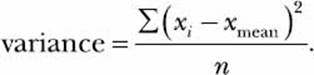
In the formula, x_i stands for individual numbers (in this case, daily total donations), x_mean stands for the mean of these numbers (the mean daily donation), and n is the number of values in the list (the number of days on which donations were received). For each value in the list, we take the difference between that number and the mean and square it. Then, we add all those squared differences together and, finally, divide the whole sum by n to find the variance.

If we want to calculate the standard deviation as well, all we have to do is take the square root of the variance. Values that are within one standard deviation of the mean can be thought of as fairly typical, whereas values that are three or more standard deviations away from the mean can be considered much more atypical—we call such values outliers.

Why do we have these two measures of dispersion—variance and standard deviation? In short, the two measures are useful in different situations. Going back to the formula we used to calculate the variance, you can see that the variance is expressed in square units because it’s the average of the squared difference from the mean. For some mathematical formulas, it’s nicer to work with those square units instead of taking the square root to find the standard deviation. On the other hand, the standard deviation is expressed in the same units as the population data. For example, if you calculate the variance for our list of donations (as we will in a moment), the result is expressed in dollars squared, which doesn’t make a lot of sense. Meanwhile, the standard deviation is simply expressed in dollars, the same unit as each of the donations.

The following program finds the variance and standard deviation for a list of numbers:

'''
Find the variance and standard deviation of a list of numbers
'''

def calculate_mean(numbers):
s = sum(numbers)
N = len(numbers)
# Calculate the mean
mean = s/N

return mean

def find_differences(numbers):
# Find the mean
mean = calculate_mean(numbers)
# Find the differences from the mean
diff = []
for num in numbers:
diff.append(num-mean)

return diff

def calculate_variance(numbers):

# Find the list of differences
➊ diff = find_differences(numbers)
# Find the squared differences
squared_diff = []
➋ for d in diff:
squared_diff.append(d**2)
# Find the variance
sum_squared_diff = sum(squared_diff)
➌ variance = sum_squared_diff/len(numbers)
return variance

if __name__ == '__main__':
donations = [100, 60, 70, 900, 100, 200, 500, 500, 503, 600, 1000, 1200]
variance = calculate_variance(donations)
print('The variance of the list of numbers is {0}'.format(variance))

➍ std = variance**0.5
print('The standard deviation of the list of numbers is {0}'.format(std))

The function calculate_variance() calculates the variance of the list of numbers passed to it. First, it calls the find_differences() function at ➊ to calculate the difference of each of the numbers from the mean. The find_differences() function returns the difference of each donation from the mean value as a list. In this function, we use the calculate_mean() function we wrote earlier to find the mean donation. Then, starting at ➋, the squares of these differences are calculated and saved in a list labeled squared_diff. Next, we use the sum() function to find the sum of the squared differences and, finally, calculate the variance at ➌. At ➍, we calculate the standard deviation by taking the square root of the variance.

When you run the preceding program, you should see the following output:

The variance of the list of numbers is 141047.35416666666
The standard deviation of the list of numbers is 375.5627166887931

The variance and the standard deviation are both very large, meaning that the individual daily total donations vary greatly from the mean. Now, let’s compare the variance and the standard deviation for a different set of donations that have the same mean: 382, 389, 377, 397, 396, 368, 369, 392, 398, 367, 393, and 396. In this case, the variance and the standard deviation turn out to be 135.38888888888889 and 11.63567311713804, respectively. Lower values for variance and standard deviation tell us that the individual numbers are closer to the mean. Figure 3-1 illustrates this point visually.

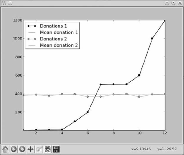
Figure 3-1: Variation of the donations around the average donation

The mean donations for both lists of donations are similar, so the two lines overlap, appearing as a single line in the figure. However, the donations from the first list vary widely from the mean, whereas the donations from the second list are very close to the mean, which confirms what we inferred from the lower variance value.

Calculating the Correlation Between Two Data Sets

In this section, we’ll learn how to calculate a statistical measure that tells us the nature and strength of the relationship between two sets of numbers: the Pearson correlation coefficient, which I’ll call simply the correlation coefficient. Note that this coefficient measures the strength of thelinear relationship. We’d have to use other measures (which we won’t be discussing here) to find out the coefficient when two sets have a nonlinear relationship. The coefficient can be either positive or negative, and its magnitude can range between -1 and 1 (inclusive).

A correlation coefficient of 0 indicates that there’s no linear correlation between the two quantities. (Note that this doesn’t mean the two quantities are independent of each other. There could still be a nonlinear relationship between them, for example). A coefficient of 1 or close to 1 indicates that there’s a strong positive linear correlation; a coefficient of exactly 1 is referred to as perfect positive correlation. Similarly, a correlation coefficient of -1 or close to -1 indicates a strong negative correlation, where 1 indicates a perfect negative correlation.

CORRELATION AND CAUSATION

In statistics, you’ll often come across the statement “correlation doesn’t imply causation.” This is a reminder that even if two sets of observations are strongly correlated with each other, that doesn’t mean one variable causes the other. When two variables are strongly correlated, sometimes there’s a third factor that influences both variables and explains the correlation. A classic example is the correlation between ice cream sales and crime rates—if you track both of these variables in a typical city, you’re likely to find a correlation, but this doesn’t mean that ice cream sales cause crime (or vice versa). Ice cream sales and crime are correlated because they both go up as the weather gets hotter during the summer. Of course, this doesn’t mean that hot weather directly causes crime to go up either; there are more complicated causes behind that correlation as well.

Calculating the Correlation Coefficient

The correlation coefficient is calculated using the formula

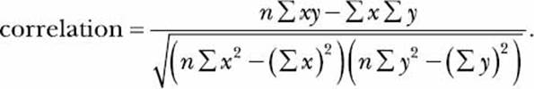
In the above formula, n is the total number of values present in each set of numbers (the sets have to be of equal length). The two sets of numbers are denoted by x and y (it doesn’t matter which one you denote as which). The other terms are described as follows:

Once we’ve calculated these terms, you can combine them according to the preceding formula to find the correlation coefficient. For small lists, it’s possible to do this by hand without too much effort, but it certainly gets complicated as the size of each set of numbers increases.

In a moment, we’ll write a program that calculates the correlation coefficient for us. In this program, we’ll use the zip() function, which will help us calculate the sum of products from the two sets of numbers. Here’s an example of how the zip() function works:

>>> simple_list1 = [1, 2, 3]
>>> simple_list2 = [4, 5, 6]
>>> for x, y in zip(simple_list1, simple_list2):
print(x, y)

1 4
2 5
3 6

The zip() function returns pairs of the corresponding elements in x and y, which you can then use in a loop to perform other operations (like printing, as shown in the preceding code). If the two lists are unequal in length, the function terminates when all the elements of the smaller list have been read.

Now we’re ready to write a program that will calculate the correlation coefficient for us:

def find_corr_x_y(x,y):
n = len(x)

# Find the sum of the products
prod = []
➊ for xi,yi in zip(x,y):
prod.append(xi*yi)

➋ sum_prod_x_y = sum(prod)
➌ sum_x = sum(x)
➍ sum_y = sum(y)
squared_sum_x = sum_x**2
squared_sum_y = sum_y**2

x_square = []
➎ for xi in x:
x_square.append(xi**2)
# Find the sum
x_square_sum = sum(x_square)

y_square=[]
for yi in y:
y_square.append(yi**2)
# Find the sum
y_square_sum = sum(y_square)

# Use formula to calculate correlation
➏ numerator = n*sum_prod_x_y - sum_x*sum_y
denominator_term1 = n*x_square_sum - squared_sum_x
denominator_term2 = n*y_square_sum - squared_sum_y
➐ denominator = (denominator_term1*denominator_term2)**0.5
➑ correlation = numerator/denominator

return correlation

The find_corr_x_y() function accepts two arguments, x and y, which are the two sets of numbers we want to calculate the correlation for. At the beginning of this function, we find the length of the lists and create a label, n, to refer to it. Next, at ➊, we have a for loop that uses the zip()function to calculate the product of the corresponding values from each list (multiplying together the first item of each list, then the second item of each list, and so on). We use the append() method to add these products to the list labeled prod.

At ➋, we calculate the sum of the products stored in prod using the sum() function. In the statements at ➌ and ➍, we calculate the sum of the numbers in x and y, respectively (once again, using the sum() function). Then, we calculate the squares of the sum of the elements in x and y, creating the labels squared_sum_x and squared_sum_y to refer to them, respectively.

In the loop starting at ➎, we calculate the square of each of the elements in x and find the sum of these squares. Then, we do the same for the elements in y. We now have all the terms we need to calculate the correlation, and we do this in the statements at ➏, ➐, and ➑. Finally, we return the correlation. Correlation is an oft-cited measure in statistical studies—in popular media and scientific articles alike. Sometimes we know ahead of time that there’s a correlation, and we just want to find the strength of that correlation. We’ll see an example of this in “Reading Data from a CSV File” on page 86, when we calculate the correlation between data read from a file. Other times, we might only suspect that there might be a correlation, and we must investigate the data to verify whether there actually is one (as in the following example).

High School Grades and Performance on College Admission Tests

In this section, we’ll consider a fictional group of 10 students in high school and investigate whether there’s a relationship between their grades in school and how they fared on their college admission tests. Table 3-2 lists the data we’re going to assume for our study and base our experiments on. The “High school grades” column lists the percentile scores of the students’ grades in high school, and the “College admission test scores” column shows their percentile scores on the college admission test.

Table 3-2: High School Grades and College Admission Test Performance

To analyze this data, let’s look at a scatter plot. Figure 3-2 shows the scatter plot of the preceding data set, with the x-axis representing high school grades and the y-axis representing the corresponding college admission test performance.

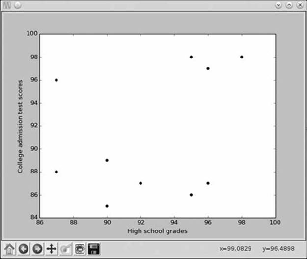
Figure 3-2: Scatter plot of high school grades and college admission test scores

The plot of the data indicates that the students with the highest grades in high school didn’t necessarily perform better on the college admission tests and vice versa. Some students with poor high school grades did very well on the college entrance exam, while others had excellent grades but did relatively poorly on the college exam. If we calculate the correlation coefficient of the two data sets (using our program from earlier), we see that it’s approximately 0.32. This means that there’s some correlation, but not a very strong one. If the correlation were closer to 1, we’d see this reflected in the scatter plot as well—the points would conform more closely to a straight, diagonal line.

Let’s assume that the high school grades shown in Table 3-2 are an average of individual grades in math, science, English, and social science. Let’s also imagine that the college exam places a high emphasis on math—much more so than on other subjects. Instead of looking at students’ overall high school grades, let’s look at just their grades in math to see whether that’s a better predictor of how they did on their college exam. Table 3-3 now shows only the math scores (as percentiles) and the college admission tests. The corresponding scatter plot is shown in Figure 3-3.

Table 3-3: High School Math Grades and College Admission Test Performance

Now, the scatter plot (Figure 3-3) shows the data points lying almost perfectly along a straight line. This is an indication of a high correlation between the high school math scores and performance on the college admission test. The correlation coefficient, in this case, turns out to be approximately 1. With the help of the scatter plot and correlation coefficient, we can conclude that there is indeed a strong relationship in this data set between grades in high school math and performance on college admission tests.

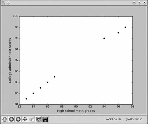
Figure 3-3: Scatter plot of high school math grades and college admission test scores

Scatter Plots

In the previous section, we saw an example of how a scatter plot can give us a first indication of the existence of any correlation between two sets of numbers. In this section, we’ll see the importance of analyzing scatter plots by looking at a set of four data sets. For these data sets, conventional statistical measures all turn out to be the same, but the scatter plots of each data set reveal important differences.

First, let’s go over how to create a scatter plot in Python:

>>> x = [1, 2, 3, 4]
>>> y = [2, 4, 6, 8]
>>> import matplotlib.pyplot as plt
➊ >>> plt.scatter(x, y)
<matplotlib.collections.PathCollection object at 0x7f351825d550>
>>> plt.show()

The scatter() function is used to create a scatter plot between two lists of numbers, x and y ➊. The only difference between this plot and the plots we created in Chapter 2 is that here we use the scatter() function instead of the plot() function. Once again, we have to call show() to display the plot.

To learn more about scatter plots, let’s look at an important statistical study: “Graphs in Statistical Analysis” by the statistician Francis Anscombe.¹ The study considers four different data sets—referred to as Anscombe’s quartet—with identical statistical properties: mean, variance, and correlation coefficient.

The data sets are as shown in Table 3-4 (reproduced from the original study).

Table 3-4: Anscombe’s Quartet—Four Different Data Sets with Almost Identical Statistical Measures

We’ll refer to the pairs (X1, Y1), (X2, Y2), (X3, Y3), and (X4, Y4) as data sets A, B, C, and D, respectively. Table 3-5 presents the statistical measures of the data sets rounded off to two decimal digits.

Table 3-5: Anscombe’s Quartet—Statistical Measures

The scatter plots for each data set are shown in Figure 3-4.

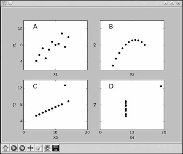
Figure 3-4: Scatter plots of Anscombe’s quartet

If we look at just the traditional statistical measures (see Table 3-5)— like the mean, standard deviation, and correlation coefficient—these data sets seem nearly identical. But the scatter plots show that these data sets are actually quite different from each other. Thus, scatter plots can be an important tool and should be used alongside other statistical measures before drawing any conclusions about a data set.

Reading Data from Files

In all our programs in this chapter, the lists of numbers we used in our calculations were all explicitly written, or hardcoded, into the programs themselves. If you wanted to find the measures for a different data set, you’d have to enter the entire new data set in the program itself. You also know how to make programs that allow the user to enter the data as input, but with large data sets, it isn’t very convenient to make the user enter long lists of numbers each time he or she uses the program.

A better alternative is to read the user data from a file. Let’s see a simple example of how we can read numbers from a file and perform mathematical operations on them. First, I’ll show how to read data from a simple text file with each line of the file containing a new data element. Then, I’ll show you how to read from a file where the data is stored in the well-known CSV format, which will open up a lot of possibilities as there are loads of useful data sets you can download from the Internet in CSV format. (If you aren’t familiar with file handling in Python, see Appendix Bfor a brief introduction.)

Reading Data from a Text File

Let’s take a file, mydata.txt, with the list of donations (one per line) during period A that we considered at the beginning of this chapter:

100
60
70
900
100
200
500
500
503
600
1000
1200

The following program will read this file and print the sum of the numbers stored in the file:

# Find the sum of numbers stored in a file
def sum_data(filename):
s = 0
➊ with open(filename) as f:
for line in f:
➋ s = s + float(line)
print('Sum of the numbers: {0}'.format(s))

if __name__ == '__main__':
sum_data('mydata.txt')

The sum_data() function opens the file specified by the argument filename at ➊ and reads it line by line (f is referred to as the file object, and you can think of it as pointing to an opened file). At ➋, we convert each number to a floating point number using the float() function and then keep adding until we’ve read all the numbers. The final number, labeled s, holds the sum of the numbers, which is printed at the end of the function.

Before you run the program, you must first create a file called mydata.txt with the appropriate data and save it in the same directory as your program. You can create this file from IDLE itself by clicking File▸New Window, typing the numbers (one per line) in the new window, and then saving the file as mydata.txt in the same directory as your program. Now, if you run the program, you’ll see the following output:

Sum of the numbers: 5733.0

All our programs in this chapter have assumed that the input data is available in lists. To use our earlier programs on the data from a file, we need to first create a list from that data. Once we have a list, we can use the functions we wrote earlier to calculate the corresponding statistic. The following program calculates the mean of the numbers stored in the file mydata.txt:

'''
Calculating the mean of numbers stored in a file
'''
def read_data(filename):

numbers = []
with open(filename) as f:
for line in f:
➊ numbers.append(float(line))

return numbers

def calculate_mean(numbers):
s = sum(numbers)
N = len(numbers)
mean = s/N

return mean

if __name__ == '__main__':
➋ data = read_data('mydata.txt')
mean = calculate_mean(data)
print('Mean: {0}'.format(mean))

Before we can call the calculate_mean() function, we need to read the numbers stored in the file and convert them into a list. To do this, use the read_data() function, which reads the file line by line. Instead of summing the numbers, this function converts them into floating point numbers and adds them to the list numbers ➊. The list is returned, and we refer to it by the label data ➋. We then invoke the calculate_mean() function, which returns the mean of the data. Finally, we print it.

When you run the program, you should see the following output:

Mean: 477.75

Of course, you’ll see a different value for the mean if the numbers in your file are different from those in this example.

See Appendix B for hints on how you can ask the user to input the filename and then modify your program accordingly. This will allow your program’s user to specify any data file.

Reading Data from a CSV File

A comma-separated value (CSV) file consists of rows and columns with the columns separated from each other by commas. You can view a CSV file using a text editor on your operating system or specialized software, such as Microsoft Excel, OpenOffice Calc, or LibreOffice Calc.

Here’s a sample CSV file containing a few numbers and their squares:

Number,Squared
10,100
9,81
22,484

The first line is referred to as the header. In this case, it tells us that the entries in the first column of this file are numbers and those in the second column are the corresponding squares. The next three lines, or rows, contain a number and its square separated by a comma. It’s possible to read the data from this file using an approach similar to what I showed for the .txt file. However, Python’s standard library has a dedicated module (csv) for reading (and writing) CSV files, which makes things a little easier.

Save the numbers and their squares into a file, numbers.csv, in the same directory as your programs. The following program shows how to read this file and then create a scatter plot displaying the numbers against their squares:

import csv
import matplotlib.pyplot as plt

def scatter_plot(x, y):
plt.scatter(x, y)
plt.xlabel('Number')
plt.ylabel('Square')
plt.show()

def read_csv(filename):

numbers = []
squared = []
with open(filename) as f:
➊ reader = csv.reader(f)
next(reader)
➋ for row in reader:
numbers.append(int(row[0]))
squared.append(int(row[1]))
return numbers, squared

if __name__ == '__main__':
numbers, squared = read_csv('numbers.csv')
scatter_plot(numbers, squared)

The read_csv() function reads the CSV file using the reader() function defined in the csv module (which is imported at the beginning of the program). This function is called with the file object f passed to it as an argument ➊. This function then returns a pointer to the first line of the CSV file. We know that the first line of the file is the header, which we want to skip, so we move the pointer to the next line using the next() function. We then read every line of the file with each line referred to by the label row ➋, with row[0] referring to the first column of the data and row[1]referring to the second. For this specific file, we know that both these numbers are integers, so we use the int() function to convert these from strings to integers and to store them in two lists. The lists are then returned—one containing the numbers and the other containing the squares.

We then call the scatter_plot() function with these two lists to create the scatter plot. The find_corr_x_y() function we wrote earlier can also easily be used to find the correlation coefficient between the two sets of numbers.

Now let’s try dealing with a more complex CSV file. Open https://www.google.com/trends/correlate/ in your browser, enter any search query you wish to (for example, summer), and click the Search correlations button. You’ll see that a number of results are returned under the heading “Correlated with summer,” and the first result is the one with the highest correlation (the number on the immediate left of each result). Click the Scatter plot option above the graph to see a scatter plot with the x-axis labeled summer and the y-axis labeled with the top result. Ignore the exact numbers plotted on both axes as we’re interested only in the correlation and the scatter plot.

A little above the scatterplot, click Export data as CSV and a file download will start. Save this file in the same directory as your programs.

This CSV file is slightly different from the one we saw earlier. At the beginning of the file, you’ll see a number of blank lines and lines with a '#' symbol until finally you’ll see the header and the data. These lines aren’t useful to us—go ahead and delete them by hand using whatever software you opened the file with so that the first line of the file is the header. Also delete any blank lines at the end of the file. Now save the file. This step— where we cleaned up the file to make it easier to process with Python—is usually called preprocessing the data.

The header has several columns. The first contains the date of the data in each row (each row has data corresponding to the week that started on the date in this column). The second column is the search query you entered, the third column shows the search query with the highestcorrelation with your search query, and the other columns include a number of other search queries arranged in decreasing order of correlation with your entered search query. The numbers in these columns are the z-scores of the corresponding search queries. The z-score indicates the difference between the number of times a term was searched for during a specific week and the overall mean number of searches per week for that term. A positive z-score indicates that the number of searches was higher than the mean for that week, and a negative z-score indicates it was lower.

For now, let’s just work with the second and the third columns. You could use the following read_csv() function to read these columns:

def read_csv(filename):

with open(filename) as f:
reader = csv.reader(f)
next(reader)

summer = []
highest_correlated = []
➊ for row in reader:
summer.append(float(row[1]))
highest_correlated.append(float(row[2]))

return summer, highest_correlated

This is pretty much like the earlier version of the read_csv function; the main change here is how we append the values to each list starting at ➊: we’re now reading the second and the third members of each row, and we’re storing them as floating point numbers.

The following program uses this function to calculate the correlation between the values for the search query you provided and the values for the query with the highest correlation with it. It also creates a scatter plot of these values:

import matplotlib.pyplot as plt
import csv

if __name__ == '__main__':
➊ summer, highest_correlated = read_csv('correlate-summer.csv')
corr = find_corr_x_y(summer, highest_correlated)
print('Highest correlation: {0}'.format(corr))
scatter_plot(summer, highest_correlated)

Assuming that the CSV file was saved as correlate-summer.csv, we call the read_csv() function to read the data in the second and third columns ➊. Then, we call the find_corr_x_y() function we wrote earlier with the two lists summer and highest_correlated. It returns the correlation coefficient, which we then print. Now, we call the scatter_plot() function we wrote earlier with these two lists again. Before you can run this program, you’ll need to include the definitions of the read_csv(), find_corr_x_y(), and scatter_plot() functions.

On running, you’ll see that it prints the correlation coefficient and also creates a scatter plot. Both of these should be very similar to the data shown on the Google correlate website.

What You Learned

In this chapter, you learned to calculate statistical measures to describe a set of numbers and the relationships between sets of numbers. You also used graphs to aid your understanding of these measures. You learned a number of new programming tools and concepts while writing programs to calculate these measures.

Programming Challenges

Next, apply what you’ve learned to complete the following programming challenges.

#1: Better Correlation Coefficient-Finding Program

The find_corr_x_y() function we wrote earlier to find the correlation co efficient between two sets of numbers assumes that the two sets of numbers are the same length. Improve the function so that it first checks the length of the lists. If they’re equal, only then should the function proceed with the remaining calculations; otherwise, it should print an error message that the correlation can’t be found.

#2: Statistics Calculator

Implement a statistics calculator that takes a list of numbers in the file mydata.txt and then calculates and prints their mean, median, mode, variance, and standard deviation using the functions we wrote earlier in this chapter.

#3: Experiment with Other CSV Data

You can experiment with numerous interesting data sources freely available on the Internet. The website http://www.quandl.com/ is one such source. For this challenge, download the following data as a CVS file from http://www.quandl.com/WORLDBANK/USA_SP_POP_TOTL/: the total population of the United States at the end of each year for the years 1960 to 2012. Then, calculate the mean, median, variance, and standard deviation of the difference in population over the years and create a graph showing these differences.

#4: Finding the Percentile

The percentile is a commonly used statistic that conveys the value below which a given percentage of observations falls. For example, if a student obtained a 95 percentile score on an exam, this means that 95 percent of the students scored less than or equal to the student’s score. For another example, in the list of numbers 5, 1, 9, 3, 14, 9, and 7, the 50th percentile is 7 and the 25th percentile is 3.5, a number that is not present in the list.

There are a number of ways to find the observation corresponding to a given percentile, but here’s one approach.²

Let’s say we want to calculate the observation at percentile p:

1. In ascending order, sort the given list of numbers, which we might call data.

2. Calculate

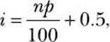
where n is the number of items in data.

3. If i is an integer, data[i] is the number corresponding to percentile p.

4. If i is not an integer, set k equal to the integral part of i and f equal to the fractional part of i. The number (1-f)*data[k] + f*data[k+1] is the number at percentile p.

Using this approach, write a program that will take a set of numbers in a file and display the number that corresponds to a specific percentile supplied as an input to the program.

#5: Creating a Grouped Frequency Table

For this challenge, your task is to write a program that creates a grouped frequency table from a set of numbers. A grouped frequency table displays the frequency of data classified into different classes. For example, let’s consider the scores we discussed in “Creating a Frequency Table” onpage 69: 7, 8, 9, 2, 10, 9, 9, 9, 9, 4, 5, 6, 1, 5, 6, 7, 8, 6, 1, and 10. A grouped frequency table would display this data as follows:

The table classifies the grades into two classes: 1-6 (which includes 1 but not 6) and 6-11 (which includes 6 but not 11). It displays against them the number of grades that belong to each category. Determining the number of classes and the range of numbers in each class are two key steps involved in creating this table. In this example, I’ve demonstrated two classes with the range of numbers in each class equally divided between the two.

Here’s one simple approach to creating classes, which assumes the number of classes can be arbitrarily chosen:

def create_classes(numbers, n):
low = min(numbers)
high = max(numbers)

# Width of each class
width = (high - low)/n
classes = []
a = low
b = low + width
classes = []
while a < (high-width):
classes.append((a, b))
a = b
b = a + width
# The last class may be of a size that is less than width
classes.append((a, high+1))
return classes

The create_classes() function accepts two arguments: a list of numbers, numbers, and n, the number of classes to create. It’ll return a list of tuples with each tuple representing a class. For example, if it’s called with numbers 7, 8, 9, 2, 10, 9, 9, 9, 9, 4, 5, 6, 1, 5, 6, 7, 8, 6, 1, 10, and n = 4, it returns the following list: [(1, 3.25), (3.25, 5.5), (5.5, 7.75), (7.75, 11)]. Once you have the list, the next step is to go over each of the numbers and find out which of the returned classes it belongs to.

Your challenge is to write a program to read a list of numbers from a file and then to print the grouped frequency table, making use of the create_classes() function.