DOING MATH WITH PYTHON Use Programming to Explore Algebra, Statistics, Calculus, and More! (2015)
6
Drawing Geometric Shapes and Fractals

In this chapter, we’ll start by learning about patches in matplotlib that allow us to draw geometric shapes, such as circles, triangles, and polygons. We’ll then learn about matplotlib’s animation support and write a program to animate a projectile’s trajectory. In the final section, we’ll learn how to draw fractals—complex geometric shapes created by the repeated applications of simple geometric transformations. Let’s get started!
Drawing Geometric Shapes with Matplotlib’s Patches
In matplotlib, patches allow us to draw geometric shapes, each of which we refer to as a patch. You can specify, for example, a circle’s radius and center in order to add the corresponding circle to your plot. This is quite different from how we’ve used matplotlib so far, which has been to supply the x- and y-coordinates of the points to plot. Before we can write a program to make use of the patches feature, however, we’ll need to understand a little bit more about how a matplotlib plot is created. Consider the following program, which plots the points (1, 1), (2, 2), and (3, 3) using matplotlib:
>>> import matplotlib.pyplot as plt
>>> x = [1, 2, 3]
>>> y = [1, 2, 3]
>>> plt.plot(x, y)
[<matplotlib.lines.Line2D object at 0x7fe822d67a20>]
>>> plt.show()
This program creates a matplotlib window that shows a line passing through the given points. Under the hood, when the plt.plot() function is called, a Figure object is created, within which the axes are created, and finally the data is plotted within the axes (see Figure 6-1).1
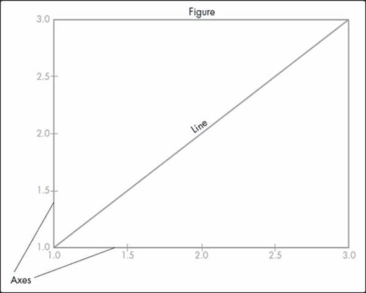
Figure 6-1: Architecture of a matplotlib plot
The following program re-creates this plot, but we’ll also explicitly create the Figure object and add axes to it, instead of just calling the plot() function and relying on it to create those:
>>> import matplotlib.pyplot as plt
>>> x = [1, 2, 3]
>>> y = [1, 2, 3]
➊ >>> fig = plt.figure()
➋ >>> ax = plt.axes()
>>> plt.plot(x, y)
[<matplotlib.lines.Line2D object at 0x7f9bad1dcc18>]
>>> plt.show()
>>>
Here, we create the Figure object using the figure() function at ➊, and then we create the axes using the axes() function at ➋. The axes() function also adds the axes to the Figure object. The last two lines are the same as in the earlier program. This time, when we call the plot() function, it sees that a Figure object with an Axes object already exists and directly proceeds to plot the data supplied to it.
Besides manually creating Figure and Axes objects, you can use two different functions in the pyplot module to get a reference to the current Figure and Axes objects. When you call the gcf() function, it returns a reference to the current Figure, and when you call the gca() function, it returns a reference to the current Axes. An interesting feature of these functions is that each will create the respective object if it doesn’t already exist. How these functions work will become clearer as we make use of them later in this chapter.
Drawing a Circle
To draw a circle, you can add the Circle patch to the current Axes object, as demonstrated by the following example:
'''
Example of using matplotlib's Circle patch
'''
import matplotlib.pyplot as plt
def create_circle():
➊ circle = plt.Circle((0, 0), radius = 0.5)
return circle
def show_shape(patch):
➋ ax = plt.gca()
ax.add_patch(patch)
plt.axis('scaled')
plt.show()
if __name__ == '__main__':
➌ c = create_circle()
show_shape(c)
In this program, we’ve separated the creation of the Circle patch object and the addition of the patch to the figure into two functions: create_circle() and show_shape(). In create_circle(), we make a circle with a center at (0, 0) and a radius of 0.5 by creating a Circle object with the coordinates of the center (0, 0) passed as a tuple and with the radius of 0.5 passed using the keyword argument of the same name at ➊. The function returns the created Circle object.
The show_shape() function is written such that it will work with any matplotlib patch. It first gets a reference to the current Axes object using the gca() function at ➋. Then, it adds the patch passed to it using the add_patch() function and, finally, calls the show() function to display the figure. We call the axis() function here with the scaled parameter, which basically tells matplotlib to automatically adjust the axis limits. We’ll need to have this statement in all programs that use patches to automatically scale the axes. You can, of course, also specify fixed values for the limits, as we saw in Chapter 2.
At ➌, we call the create_circle() function using the label c to refer to the returned Circle object. Then, we call the show_shape() function, passing c as an argument. When you run the program, you’ll see a matplotlib window showing the circle (see Figure 6-2).
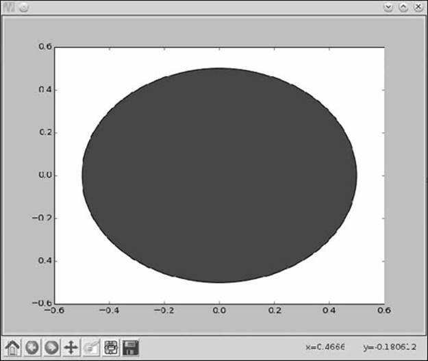
Figure 6-2: A circle with a center of (0, 0) and radius of 0.5
The circle doesn’t quite look like a circle here, as you can see. This is due to the automatic aspect ratio, which determines the ratio of the length of the x- and y-axes. If you insert the statement ax.set_aspect('equal') after ➋, you will see that the circle does indeed look like a circle. Theset_aspect() function is used to set the aspect ratio of the graph; using the equal argument, we ask matplotlib to set the ratio of the length of the x- and y-axes to 1:1.
Both the edge color and the face color (fill color) of the patch can be changed using the ec and fc keyword arguments. For example, passing fc='g' and ec='r' will create a circle with a green face color and red edge color.
Matplotlib supports a number of other patches, such as Ellipse, Polygon, and Rectangle.
Creating Animated Figures
Sometimes we may want to create figures with moving shapes. Matplotlib’s animation support will help us achieve this. At the end of this section, we’ll create an animated version of the projectile trajectory-drawing program.
First, let’s see a simpler example. We’ll draw a matplotlib figure with a circle that starts off small and grows to a certain radius indefinitely (unless the matplotlib window is closed):
'''
A growing circle
'''
from matplotlib import pyplot as plt
from matplotlib import animation
def create_circle():
circle = plt.Circle((0, 0), 0.05)
return circle
def update_radius(i, circle):
circle.radius = i*0.5
return circle,
def create_animation():
➊ fig = plt.gcf()
ax = plt.axes(xlim=(-10, 10), ylim=(-10, 10))
ax.set_aspect('equal')
circle = create_circle()
➋ ax.add_patch(circle)
➌ anim = animation.FuncAnimation(
fig, update_radius, fargs = (circle,), frames=30, interval=50)
plt.title('Simple Circle Animation')
plt.show()
if __name__ == '__main__':
create_animation()
We start by importing the animation module from the matplotlib package. The create_animation() function carries out the core functionality here. It gets a reference to the current Figure object using the gcf() function at ➊ and then creates the axes with limits of -10 and 10 for both the x- and y-axes. After that, it creates a Circle object that represents a circle with a radius of 0.05 and a center at (0, 0) and adds this circle to the current axes at ➋. Then, we create a FuncAnimation object ➌, which passes the following data about the animation we want to create:
fig This is the current Figure object.
update_radius This function will be responsible for drawing every frame. It takes two arguments—a frame number that is automatically passed to it when called and the patch object that we want to update every frame. This function also must return the object.
fargs This tuple consists of all the arguments to be passed to the update_radius() function other than the frame number. If there are no such arguments to pass, this keyword argument need not be specified.
frames This is the number of frames in the animation. Our function update_radius() is called this many times. Here, we’ve arbitrarily chosen 30 frames.
interval This is the time interval in milliseconds between two frames. If your animation seems too slow, decrease this value; if it seems too fast, increase this value.
We then set a title using the title() function and, finally, show the figure using the show() function.
As mentioned earlier, the update_radius() function is responsible for updating the property of the circle that will change each frame. Here, we set the radius to i*0.5, where i is the frame number. As a result, you see a circle that grows every frame for 30 frames—thus, the radius of the largest circle is 15. Because the axes’ limits are set at -10 and 10, this gives the effect of the circle exceeding the figure’s dimensions. When you run the program, you’ll see your first animated figure, as shown in Figure 6-3.
You’ll notice that the animation continues until you close the matplotlib window. This is the default behavior, which you can change by setting the keyword argument to repeat=False when you create the FuncAnimation object.
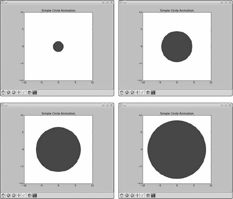
Figure 6-3: Simple circle animation
FUNCANIMATION OBJECT AND PERSISTENCE
You probably noted in the animated circle program that we assigned the created FuncAnimation object to the label anim even though we don’t use it again elsewhere. This is because of an issue with matplotlib’s current behavior—it doesn’t store any reference to the FuncAnimation object, making it subject to garbage collection by Python. This means the animation will not be created. Creating a label referring to the object prevents this from happening.
Animating a Projectile’s Trajectory
In Chapter 2, we drew the trajectory for a ball in projectile motion. Here, we’ll build upon this drawing, making use of matplotlib’s animation support to animate the trajectory so that it will come closer to demonstrating how you’d see a ball travel in real life:
'''
Animate the trajectory of an object in projectile motion
'''
from matplotlib import pyplot as plt
from matplotlib import animation
import math
g = 9.8
def get_intervals(u, theta):
t_flight = 2*u*math.sin(theta)/g
intervals = []
start = 0
interval = 0.005
while start < t_flight:
intervals.append(start)
start = start + interval
return intervals
def update_position(i, circle, intervals, u, theta):
t = intervals[i]
x = u*math.cos(theta)*t
y = u*math.sin(theta)*t - 0.5*g*t*t
circle.center = x, y
return circle,
def create_animation(u, theta):
intervals = get_intervals(u, theta)
xmin = 0
xmax = u*math.cos(theta)*intervals[-1]
ymin = 0
t_max = u*math.sin(theta)/g
➊ ymax = u*math.sin(theta)*t_max - 0.5*g*t_max**2
fig = plt.gcf()
➋ ax = plt.axes(xlim=(xmin, xmax), ylim=(ymin, ymax))
circle = plt.Circle((xmin, ymin), 1.0)
ax.add_patch(circle)
➌ anim = animation.FuncAnimation(fig, update_position,
fargs=(circle, intervals, u, theta),
frames=len(intervals), interval=1,
repeat=False)
plt.title('Projectile Motion')
plt.xlabel('X')
plt.ylabel('Y')
plt.show()
if __name__ == '__main__':
try:
u = float(input('Enter the initial velocity (m/s): '))
theta = float(input('Enter the angle of projection (degrees): '))
except ValueError:
print('You entered an invalid input')
else:
theta = math.radians(theta)
create_animation(u, theta)
The create_animation() function accepts two arguments: u and theta. These arguments correspond to the initial velocity and the angle of projection (θ), which were supplied as input to the program. The get_intervals() function is used to find the time intervals at which to calculate the x- and y-coordinates. This function is implemented by making use of the same logic we used in Chapter 2, when we implemented a separate function, frange(), to help us.
To set up the axis limits for the animation, we’ll need to find the minimum and maximum values of x and y. The minimum value for each is 0, which is the initial value for each. The maximum value of the x-coordinate is the value of the coordinate at the end of the flight of the ball, which is the last time interval in the list intervals. The maximum value of the y-coordinate is when the ball is at its highest point—that is, at ➊, where we calculate that point using the formula
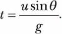
Once we have the values, we create the axes at ➋, passing the appropriate axis limits. In the next two statements, we create a representation of the ball and add it to the figure’s Axes object by creating a circle of radius 1.0 at (xmin, ymin)—the minimum coordinates of the x- and y-axes, respectively.
We then create the FuncAnimation object ➌, supplying it with the current figure object and the following arguments:
update_position This function will change the center of the circle in each frame. The idea here is that a new frame is created for every time interval, so we set the number of frames to the size of the time intervals (see the description of frames in this list). We calculate the x-and y-coordinates of the ball at the time instant at the ith time interval, and we set the center of the circle to these values.
fargs The update_position() function needs to access the list of time intervals, intervals, initial velocity, and theta, which are specified using this keyword argument.
frames Because we’ll draw one frame per time interval, we set the number of frames to the size of the intervals list.
repeat As we discussed in the first animation example, animation repeats indefinitely by default. We don’t want that to happen in this case, so we set this keyword to False.
When you run the program, it asks for the initial inputs and then creates the animation, as shown in Figure 6-4.
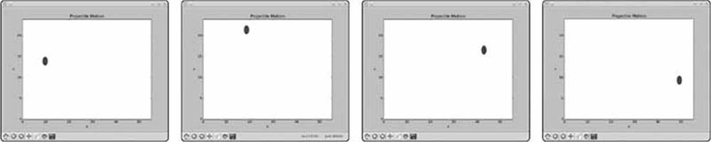
Figure 6-4: Animation of the trajectory of a projectile
Drawing Fractals
Fractals are complex geometric patterns or shapes arising out of surprisingly simple mathematical formulas. Compared to geometric shapes, such as circles and rectangles, a fractal seems irregular and without any obvious pattern or description, but if you look closely, you see that patterns emerge and the entire shape is composed of numerous copies of itself. Because fractals involve the repetitive application of the same geometric transformation of points in a plane, computer programs are well-suited to create them. In this chapter, we’ll learn how to draw the Barnsley fern, the Sierpiński triangle, and the Mandelbrot set (the latter two in the challenges)— popular examples of fractals studied in the field. Fractals abound in nature, too—popular examples include coastlines, trees, and snowflakes.
Transformations of Points in a Plane
A basic idea in creating fractals is that of the transformation of a point. Given a point, P(x, y), in an x-y plane, an example of a transformation is P (x, y) → Q (x + 1, y + 1), which means that after applying the transformation, a new point, Q, which is one unit above and one unit to the right ofP, is created. If you then consider Q as the starting point, you’ll get another point, R, that’s one unit above and one unit to the right of Q. Consider the starting point, P, to be (1, 1). Figure 6-5 shows what the points would look like.
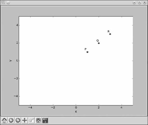
Figure 6-5: The points Q and R have been obtained by applying a transformation to the point P for two iterations.
This transformation is, thus, a rule describing how a point moves around in the x-y plane, starting from an initial position and moving to a different point at each iteration. We can think of a transformation as the point’s trajectory in the plane. Now, consider that instead of one transformation rule, there are two such rules and one of these transformations is picked at random at every step. Let’s consider these rules:
Rule 1: P 1 (x, y) → P 2 (x + 1, y - 1)
Rule 2: P 1 (x, y) → P 2 (x + 1, y + 1)
Consider P1(1, 1) to be the starting point. If we carry out four iterations, we could have the following sequence of points:
P 1 (1, 1) → P 2 (2, 0) (Rule 1)
P 2 (2, 0) → P 3 (3, 1) (Rule 2)
P 3 (3, 1) → P 4 (4, 2) (Rule 2)
P 4 (4, 2) → P 5 (5, 1) (Rule 1)
... and so on.
The transformation rule is picked at random, with each rule having an equal probability of being selected. No matter which one is picked, the points will advance toward the right because we increase the x-coordinate in both cases. As the points go to the right, they move either up or down, thus creating a zigzag path. The following program charts out the path of a point when subjected to one of these transformations for a specified number of iterations:
'''
Example of selecting a transformation from two equally probable
transformations
'''
import matplotlib.pyplot as plt
import random
def transformation_1(p):
x = p[0]
y = p[1]
return x + 1, y - 1
def transformation_2(p):
x = p[0]
y = p[1]
return x + 1, y + 1
def transform(p):
➊ # List of transformation functions
transformations = [transformation_1, transformation_2]
# Pick a random transformation function and call it
➋ t = random.choice(transformations)
➌ x, y = t(p)
return x, y
def build_trajectory(p, n):
x = [p[0]]
y = [p[1]]
for i in range(n):
p = transform(p)
x.append(p[0])
y.append(p[1])
return x, y
if __name__ == '__main__':
# Initial point
p = (1, 1)
n = int(input('Enter the number of iterations: '))
➍ x, y = build_trajectory(p, n)
# Plot
➎ plt.plot(x, y)
plt.xlabel('X')
plt.ylabel('Y')
plt.show()
We define two functions, transformation_1() and transformation_2(), corresponding to the two preceding transformations. In the transform() function, we create a list with these two function names at ➊ and use the random.choice() function to pick one of the transformations from the list at ➋. Now that we’ve picked the transformation to apply, we call it with the point, P, and store the coordinates of the transformed point in the labels x, y ➌ and return them.
SELECTING A RANDOM ELEMENT FROM A LIST
The random.choice() function we saw in our first fractal program can be used to select a random element from a list. Each element has an equal chance of being returned. Here’s an example:
>>> import random
>>> l = [1, 2, 3]
>>> random.choice(l)
3
>>> random.choice(l)
1
>>> random.choice(l)
1
>>> random.choice(l)
3
>>> random.choice(l)
3
>>> random.choice(l)
2
The function also works with tuples and strings. In the latter case, it returns a random character from the string.
When you run the program, it asks you for the number of iterations, n—that is, the number of times the transformation would be applied. Then, it calls the build_trajectory() function with n and the initial point, P, which is set to (1, 1) ➍. The build_trajectory() function repeatedly calls the transform() function n times, using two lists, x and y, to store the x-coordinate and y-coordinate of all the transformed points. Finally, it returns the two lists, which are then plotted ➎.
Figures 6-6 and 6-7 show the trajectory of the point for 100 and 10,000 iterations, respectively. The zigzag motion is quite apparent in both figures. This zigzag path is usually referred to as a random walk on a line.
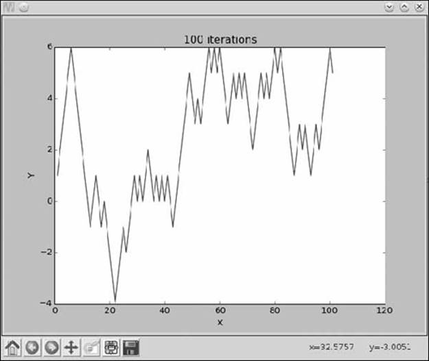
Figure 6-6: The zigzag path traced by the point (1, 1) when subjected to one or the other of the two transformations randomly for 100 iterations
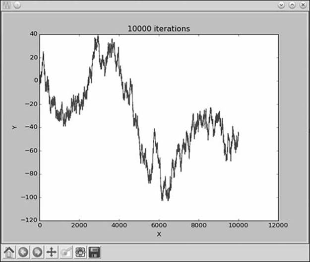
Figure 6-7: The zigzag path traced by the point (1, 1) when subjected to one or the other of the two transformations randomly for 10,000 iterations.
This example demonstrates a basic idea in creating fractals—starting from an initial point and applying a transformation to that point repeatedly. Next, we’ll see an example of applying the same ideas to draw the Barnsley fern.
Drawing the Barnsley Fern
The British mathematician Michael Barnsley described how to create fern-like structures using repeated applications of a simple transformation on a point (see Figure 6-8).
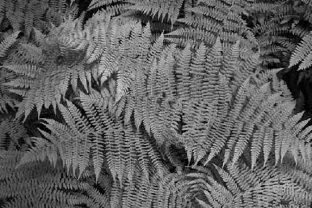
Figure 6-8: Lady ferns2
He proposed the following steps to create fern-like structures: start with the point (0, 0) and randomly select one of the following transformations with the assigned probability:
Transformation 1 (0.85 probability):
xn+1 = 0.85xn + 0.04yn
yn+1 = -0.04yn + 0.85yn + 1.6
Transformation 2 (0.07 probability):
xn+1 = 0.2xn - 0.26yn
yn+1 = 0.23yn + 0.22yn + 1.6
Transformation 3 (0.07 probability):
xn+1 = -0.15xn - 0.28xn
yn+1 = 0.26yn + 0.24yn + 0.44
Transformation 4 (0.01 probability):
xn+1 = 0
yn+1 = 0.16yn
Each of these transformations is responsible for creating a part of the fern. The first transformation selected with the highest probability—and hence the maximum number of times—creates the stem and the bottom fronds of the fern. The second and third transformations create the bottom frond on the left and the right, respectively, and the fourth transformation creates the stem of the fern.
This is an example of nonuniform probabilistic selection, which we first learned about in Chapter 5. The following program draws the Barnsley fern for the specified number of points:
'''
Draw a Barnsley Fern
'''
import random
import matplotlib.pyplot as plt
def transformation_1(p):
x = p[0]
y = p[1]
x1 = 0.85*x + 0.04*y
y1 = -0.04*x + 0.85*y + 1.6
return x1, y1
def transformation_2(p):
x = p[0]
y = p[1]
x1 = 0.2*x - 0.26*y
y1 = 0.23*x + 0.22*y + 1.6
return x1, y1
def transformation_3(p):
x = p[0]
y = p[1]
x1 = -0.15*x + 0.28*y
y1 = 0.26*x + 0.24*y + 0.44
return x1, y1
def transformation_4(p):
x = p[0]
y = p[1]
x1 = 0
y1 = 0.16*y
return x1, y1
def get_index(probability):
r = random.random()
c_probability = 0
sum_probability = []
for p in probability:
c_probability += p
sum_probability.append(c_probability)
for item, sp in enumerate(sum_probability):
if r <= sp:
return item
return len(probability)-1
def transform(p):
# List of transformation functions
transformations = [transformation_1, transformation_2,
transformation_3, transformation_4]
➊ probability = [0.85, 0.07, 0.07, 0.01]
# Pick a random transformation function and call it
tindex = get_index(probability)
➋ t = transformations[tindex]
x, y = t(p)
return x, y
def draw_fern(n):
# We start with (0, 0)
x = [0]
y = [0]
x1, y1 = 0, 0
for i in range(n):
x1, y1 = transform((x1, y1))
x.append(x1)
y.append(y1)
return x, y
if __name__ == '__main__':
n = int(input('Enter the number of points in the Fern: '))
x, y = draw_fern(n)
# Plot the points
plt.plot(x, y, 'o')
plt.title('Fern with {0} points'.format(n))
plt.show()
When you run this program, it asks for the number of points in the fern to be specified and then creates the fern. Figures 6-9 and 6-10 show ferns with 1,000 and 10,000 points, respectively.
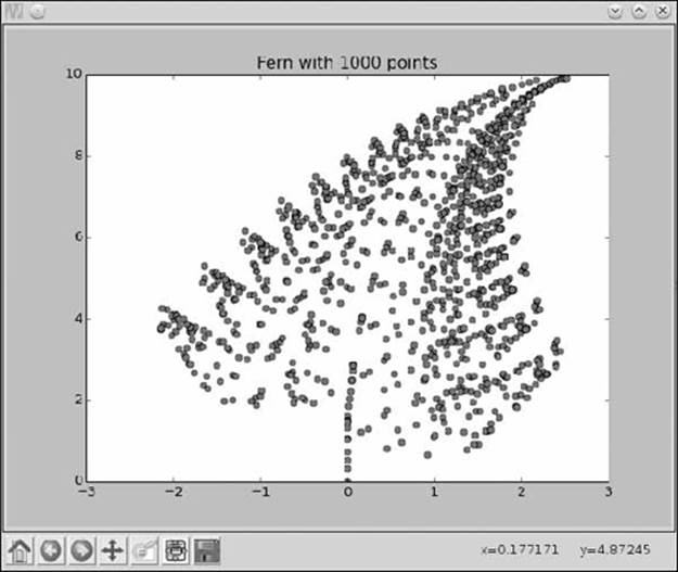
Figure 6-9: A fern with 1,000 points
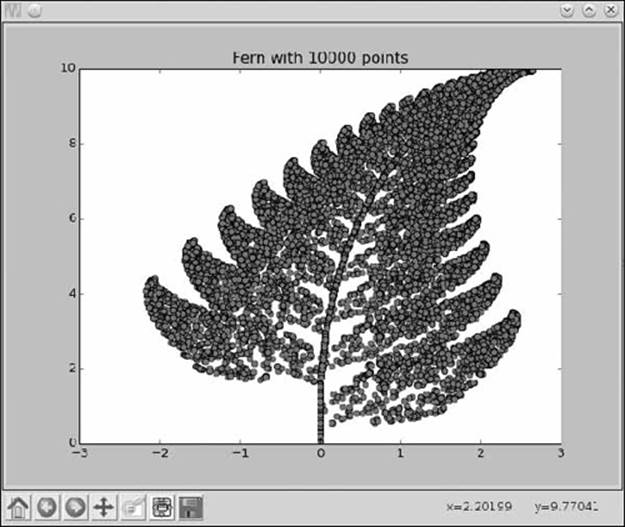
Figure 6-10: A fern with 10,000 points
The four transformation rules are defined in the transformation_1(), transformation_2(), transformation_3(), and transformation_4() functions. The probability of each being selected is declared in a list at ➊, and then one of them is selected ➋ to be applied every time the transform()function is called by the draw_fern() function.
The number of times the initial point (0, 0) is transformed is the same as the number of points in the fern specified as input to the program.
What You Learned
In this chapter, you started by learning how to draw basic geometric shapes and how to animate them. This process introduced you to a number of new matplotlib features. You then learned about geometric transformations and saw how repetitive simple transformations help you draw complex geometric shapes called fractals.
Programming Challenges
Here are a few programming challenges that should help you further apply what you’ve learned. You can find sample solutions at http://www.nostarch.com/doingmathwithpython/.
#1: Packing Circles into a Square
I mentioned earlier that matplotlib supports the creation of other geometric shapes. The Polygon patch is especially interesting, as it allows you to draw polygons with different numbers of sides. Here’s how we can draw a square (each side of length 4):
'''
Draw a square
'''
from matplotlib import pyplot as plt
def draw_square():
ax = plt.axes(xlim = (0, 6), ylim = (0, 6))
square = plt.Polygon([(1, 1), (5, 1), (5, 5), (1, 5)], closed = True)
ax.add_patch(square)
plt.show()
if __name__ == '__main__':
draw_square()
The Polygon object is created by passing the list of the vertices’ coordinates as the first argument. Because we’re drawing a square, we pass the coordinates of the four vertices: (1, 1), (5, 1), (5, 5), and (1, 5). Passing closed=True tells matplotlib that we want to draw a closed polygon, where the starting and the ending vertices are the same.
In this challenge, you’ll attempt a very simplified version of the “circles packed into a square” problem. How many circles of radius 0.5 will fit in the square produced by this code? Draw and find out! Figure 6-11 shows how the final image will look.
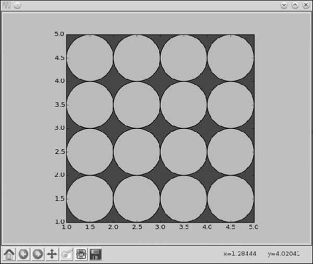
Figure 6-11: Circles packed into a square
The trick here is to start from the lower-left corner of the square— that is, (1, 1)—and then continue adding circles until the entire square is filled. The following snippet shows how you can create the circles and add them to the figure:
y = 1.5
while y < 5:
x = 1.5
while x < 5:
c = draw_circle(x, y)
ax.add_patch(c)
x += 1.0
y += 1.0
A point worth noting here is that this is not the most optimal or, for that matter, the only way to pack circles into a square, and finding different ways of solving this problem is popular among mathematics enthusiasts.
#2: Drawing the Sierpiński Triangle
The Sierpiński triangle, named after the Polish mathematician Wacław Sierpiński, is a fractal that is an equilateral triangle composed of smaller equilateral triangles embedded inside it. Figure 6-12 shows a Sierpiński triangle composed of 10,000 points.
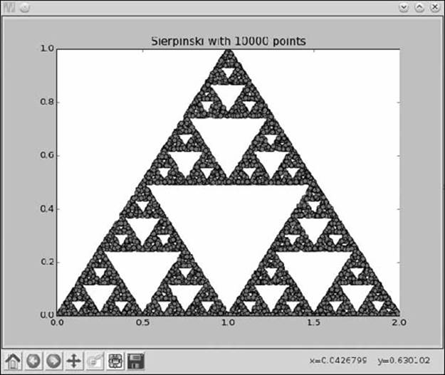
Figure 6-12: Sierpiński triangle with 10,000 points
The interesting thing here is that the same process that we used to draw a fern will also draw the Sierpiński triangle—only the transformation rules and their probability will change. Here’s how you can draw the Sierpiński triangle: start with the point (0, 0) and apply one of the following transformations:
Transformation 1:
xn+1 = 0.5xn
yn+1 = 0.5yn
Transformation 2:
xn+1 = 0.5xn + 0.5
yn+1 = 0.5yn + 0.5
Transformation 3:
xn+1 = 0.5xn + 1
yn+1 = 0.5yn
Each of the transformations has an equal probability of being selected—1/3. Your challenge here is to write a program that draws the Sierpiński triangle composed of a certain number of points specified as input.
#3: Exploring Hénon’s Function
In 1976, Michel Hénon introduced the Hénon function, which describes a transformation rule for a point P(x, y) as follows:
P (x, y) → Q (y + 1 - 1.4x2, 0.3x)
Irrespective of the initial point (provided it’s not very far from the origin), you’ll see that as you create more points, they start lying along curved lines, as shown in Figure 6-13.
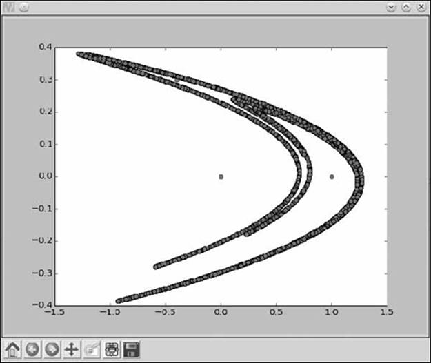
Figure 6-13: Hénon function with 10,000 points
Your challenge here is to write a program to create a graph showing 20,000 iterations of this transformation, starting with the point (1, 1).
This is an example of a dynamical system, and the curved lines that all the points seem attracted to are referred to as attractors. To learn more about this function, dynamical systems, and fractals in general, you may want to refer to Fractals: A Very Short Introduction by Kenneth Falconer (Oxford University Press, 2013).
#4: Drawing the Mandelbrot Set
Your challenge here is to write a program to draw the Mandelbrot set—another example of the application of simple rules leading to a complicated-looking shape (see Figure 6-14). Before I lay down the steps to do that, however, we’ll first learn about matplotlib’s imshow() function.
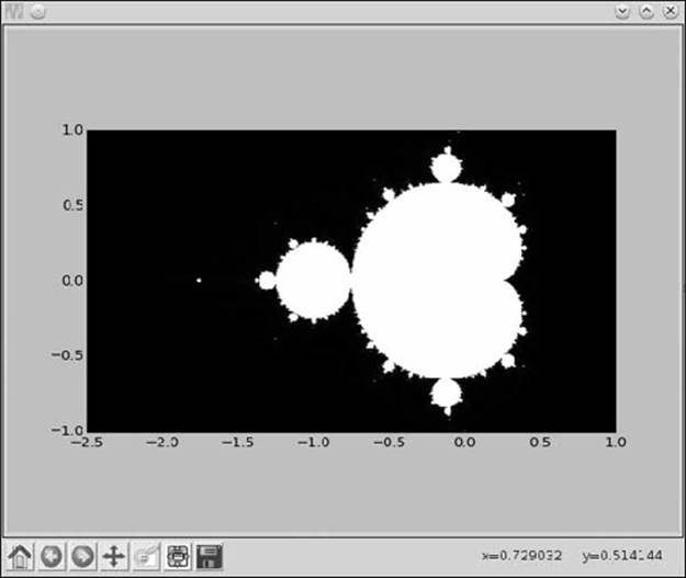
Figure 6-14: Mandelbrot set in the plane between (-2.5, -1.0) and (1.0, 1.0)
The imshow() Function
The imshow() function is usually used to display an external image, such as a JPEG or PNG image. You can see an example at http://matplotlib.org/users/image_tutorial.html. Here, however, we’ll use the function to draw a new image of our own creation via matplotlib.
Consider the part of the Cartesian plane where x and y both range from 0 to 5. Now, consider six equidistant points along each axis: (0, 1, 2, 3, 4, 5) along the x-axis and the same set of points along the y-axis. If we take the Cartesian product of these points, we get 36 equally spaced points in the x-y plane with the coordinates (0, 0), (0, 1) ... (0, 5), (1, 0), (1, 1) ... (1, 5) ... (5, 5). Let’s now say that we want to color each of these points with a shade of gray—that is, some of these points will be black, some will be white, and others will be colored with a shade in between, randomly chosen. Figure 6-15 illustrates the scenario.
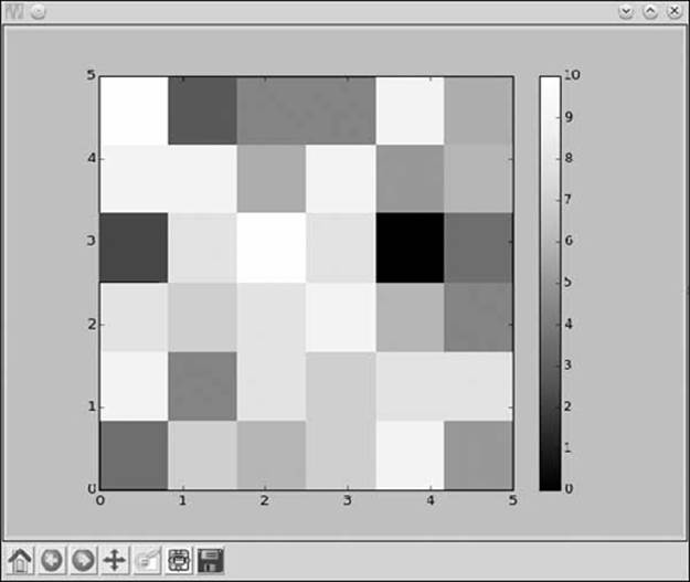
Figure 6-15: Part of the x-y plane with x and y both ranging from 0 to 5. We’ve considered 36 points in the region equidistant from each other and colored each with a shade of gray.
To create this figure, we have to make a list of six lists. Each of these six lists will in turn consist of six integers ranging from 0 to 10. Each number will correspond to the color for each point, 0 standing for black and 10 standing for white. We’ll then pass this list to the imshow() function along with other necessary arguments.
Creating a List of Lists
A list can also contain lists as its members:
>>> l1 = [1, 2, 3]
>>> l2 = [4, 5, 6]
>>> l = [l1, l2]
Here, we created a list, l, consisting of two lists, l1 and l2. The first element of the list, l[0], is thus the same as the l1 list and the second element of the list, l[1], is the same as the l2 list:
>>> l[0]
[1, 2, 3]
>>> l[1]
[4, 5, 6]
To refer to an individual element within one of the member lists, we have to specify two indices—l[0][1] refers to the second element of the first list, l[1][2] refers to the third element of the second list, and so on.
Now that we know how to work with a list of lists, we can write the program to create a figure similar to Figure 6-15:
import matplotlib.pyplot as plt
import matplotlib.cm as cm
import random
➊ def initialize_image(x_p, y_p):
image = []
for i in range(y_p):
x_colors = []
for j in range(x_p):
x_colors.append(0)
image.append(x_colors)
return image
def color_points():
x_p = 6
y_p = 6
image = initialize_image(x_p, y_p)
for i in range(y_p):
for j in range(x_p):
➋ image[i][j] = random.randint(0, 10)
➌ plt.imshow(image, origin='lower', extent=(0, 5, 0, 5),
cmap=cm.Greys_r, interpolation='nearest')
plt.colorbar()
plt.show()
if __name__ == '__main__':
color_points()
The initialize_image() function at ➊ creates a list of lists with each of the elements initialized to 0. It accepts two arguments, x_p and y_p, which correspond to the number of points along the x-axis and y-axis, respectively. This effectively means that the initialized list image will consist of x_p lists with each list containing y_p zeros.
In the color_points() function, once you have the image list back from initialize_image(), assign a random integer between 0 and 10 to the element image[i][j] at ➋. When we assign this random integer to the element, we are assigning a color to the point in the Cartesian plane that’s isteps along the y-axis and j steps along the x-axis from the origin. It’s important to note that the imshow() function automatically deduces the color of a point from its position in the image list and doesn’t care about its specific x- and y-coordinates.
Then, call the imshow() function at ➌, passing image as the first argument. The keyword argument origin='lower' specifies that the number in image[0][0] corresponds to the color of the point (0, 0). The keyword argument extent=(0, 5, 0, 5) sets the lower-left and upper-right corners of the image to (0, 0) and (5, 5), respectively. The keyword argument cmap=cm.Greys_r specifies that we’re going to create a grayscale image.
The last keyword argument, interpolation='nearest', specifies that matplotlib should color a point for which the color wasn’t specified with the same color as the one nearest to it. What does this mean? Note that we consider and specify the color for only 36 points in the region (0, 5) and (5, 5). Because there is an infinite number of points in this region, we tell matplotlib to set the color of an unspecified point to that of its nearest point. This is the reason you see color “boxes” around each point in the figure.
Call the colorbar() function to display a color bar in the figure showing which integer corresponds to which color. Finally, call show() to display the image. Note that due to the use of the random.randint() function, your image will be colored differently than the one in Figure 6-15.
If you increase the number of points along each axis by setting x_p and y_p to, let’s say, 20 in color_points(), you’ll see a figure similar to the one shown in Figure 6-16. Note that the color boxes grow smaller in size. If you increase the number of points even more, you’ll see the size of the boxes shrink further, giving the illusion that each point has a different color.
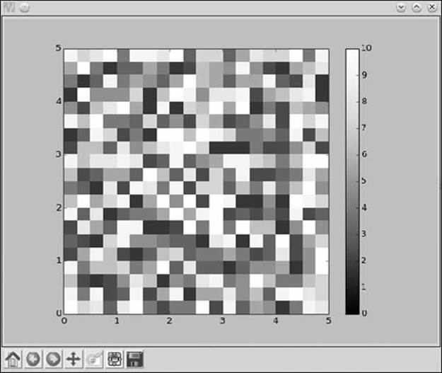
Figure 6-16: Part of the x-y plane with x and y both ranging from 0 to 5. We’ve considered 400 points in the region equidistant from each other and colored each with a shade of gray.
Drawing the Mandelbrot Set
We’ll consider the area of the x-y plane between (-2.5, -1.0) and (1.0, 1.0) and divide each axis into 400 equally spaced points. The Cartesian product of these points will give us 1,600 equally spaced points in this region. We’ll refer to these points as (x1, y1), (x1, y2) ... (x400, y400).
Create a list, image, by calling the initialize_image() function we saw earlier with both x_p and y_p set to 400. Then, follow these steps for each of the generated points (xi, yk):
1. First, create two complex numbers, z1 = 0 + 0j and c = xi + yk j. (Recall that we use j for ![]() .)
.)
2. Create a label iteration and set it to 0—that is, iteration=0.
3. Create a complex number, ![]() .
.
4. Increment the value stored in iteration by 1—that is, iteration = iteration + 1.
5. If abs(z1) < 2 and iteration < max_iteration, then go back to step 3; otherwise, go to step 6. The larger the value of max_iteration, the more detailed the image, but the longer it’ll take to create the image. Set max_iteration to 1,000 here.
6. Set the color of the point (xi, yk) to the value in iteration—that is, image[k][i] = iteration.
Once you have the complete image list, call the imshow() function with the extent keyword argument changed to indicate the region bounded by (-2.5, -1.0) and (1.0, 1.0).
This algorithm is usually referred to as the escape-time algorithm. When the maximum number of iterations is reached before a point’s magnitude exceeds 2, that point belongs to the Mandelbrot set and is colored white. The points that exceed the magnitude within fewer iterations are said to “escape”; they don’t belong to the Mandelbrot set and are colored black. You can experiment by decreasing and increasing the number of points along each axis. Decreasing the number of points will lead to a grainy image, while increasing them will result in a more detailed image.
All materials on the site are licensed Creative Commons Attribution-Sharealike 3.0 Unported CC BY-SA 3.0 & GNU Free Documentation License (GFDL)
If you are the copyright holder of any material contained on our site and intend to remove it, please contact our site administrator for approval.
© 2016-2026 All site design rights belong to S.Y.A.