Python in Practice: Create Better Programs Using Concurrency, Libraries, and Patterns (2014)
Chapter 3. Behavioral Design Patterns in Python
The behavioral patterns are concerned with how things get done; that is, with algorithms and object interactions. They provide powerful ways of thinking about and organizing computations, and like a few of the patterns seen in the previous two chapters, some of them are supported directly by built-in Python syntax.
The Perl programming language’s well-known motto is, “there’s more than one way to do it”; whereas in Tim Peters’ Zen of Python, “there should be one—and preferably only one—obvious way to do it”.* Yet, like any programming language, there are sometimes two or more ways to do things in Python, especially since the introduction of comprehensions (use a comprehension or a for loop) and generators (use a generator expression or a function with a yield statement). And as we will see in this chapter, Python’s support for coroutines adds a new way to do certain things.
*To see the Zen of Python, enter import this at an interactive Python prompt.
3.1. Chain of Responsibility Pattern
The Chain of Responsibility Pattern is designed to decouple the sender of a request from the recipient that processes the request. So, instead of one function directly calling another, the first function sends a request to a chain of receivers. The first receiver in the chain either can handle the request and stop the chain (by not passing the request on) or can pass on the request to the next receiver in the chain. The second receiver has the same choices, and so on, until the last one is reached (which could choose to throw the request away or to raise an exception).
Let’s imagine that we have a user interface that receives events to be handled. Some of the events come from the user (e.g., mouse and key events), and some come from the system (e.g., timer events). In the following two subsections we will look at a conventional approach to creating an event-handling chain, and then at a pipeline-based approach using coroutines.
3.1.1. A Conventional Chain
In this subsection we will review a conventional event-handling chain where each event has a corresponding event-handling class.
handler1 = TimerHandler(KeyHandler(MouseHandler(NullHandler())))
Here is how the chain might be set up using four separate handler classes. The chain is illustrated in Figure 3.1. Since we throw away unhandled events, we could have just passed None—or nothing—as the MouseHandler’s argument.
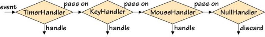
Figure 3.1 An event-handling chain
The order in which we create the handlers should not matter since each one handles events only of the type it is designed for.
while True:
event = Event.next()
if event.kind == Event.TERMINATE:
break
handler1.handle(event)
Events are normally handled in a loop. Here, we exit the loop and terminate the application if there is a TERMINATE event; otherwise, we pass the event to the event-handling chain.
handler2 = DebugHandler(handler1)
Here we have created a new handler (although we could just as easily have assigned back to handler1). This handler must be first in the chain, since it is used to eavesdrop on the events passing into the chain and to report them, but not to handle them (so it passes on every event it receives).
We can now call handler2.handle(event) in our loop, and in addition to the normal event handlers we will now have some debugging output to see the events that are received.
class NullHandler:
def __init__(self, successor=None):
self.__successor = successor
def handle(self, event):
if self.__successor is not None:
self.__successor.handle(event)
This class serves as the base class for our event handlers and provides the infrastructure for handling events. If an instance is created with a successor handler, then when this instance is given an event, it simply passes the event down the chain to the successor. However, if there is no successor, we have decided to simply discard the event. This is the standard approach in GUI (graphical user interface) programming, although we could easily log or raise an exception for unhandled events (e.g., if our program was a server).
class MouseHandler(NullHandler):
def handle(self, event):
if event.kind == Event.MOUSE:
print("Click: {}".format(event))
else:
super().handle(event)
Since we haven’t reimplemented the __init__() method, the base class one will be used, so the self.__successor variable will be correctly created.
This handler class handles only those events that it is interested in (i.e., of type Event.MOUSE) and passes any other kind of event on to its successor in the chain (if there is one).
The KeyHandler and TimerHandler classes (neither of which is shown) have exactly the same structure as the MouseHandler. These other classes only differ in which kind of event they respond to (e.g., Event.KEYPRESS and Event.TIMER) and the handling they perform (i.e., they print out different messages).
class DebugHandler(NullHandler):
def __init__(self, successor=None, file=sys.stdout):
super().__init__(successor)
self.__file = file
def handle(self, event):
self.__file.write("*DEBUG*: {}\n".format(event))
super().handle(event)
The DebugHandler class is different from the other handlers in that it never handles any events, and it must be first in the chain. It takes a file or file-like object to direct its reports to, and when an event occurs, it reports the event and then passes it on.
3.1.2. A Coroutine-Based Chain
A generator is a function or method that has one or more yield expressions instead of returns. Whenever a yield is reached, the value yielded is produced, and the function or method is suspended with all its state intact. At this point the function has yielded the processor (to the receiver of the value it has produced), so although suspended, the function does not block. Then, when the function or method is used again, execution resumes from the statement following the yield. So, values are pulled from a generator by iterating over it (e.g., using for value ingenerator:) or by calling next() on it.
A coroutine uses the same yield expression as a generator but has different behavior. A coroutine executes an infinite loop and starts out suspended at its first (or only) yield expression, waiting for a value to be sent to it. If and when a value is sent, the coroutine receives this as the value of its yield expression. The coroutine can then do any processing it wants and when it has finished, it loops and again becomes suspended waiting for a value to arrive at its next yield expression. So, values are pushed into a coroutine by calling the coroutine’s send() or throw()methods.
In Python, any function or method that contains a yield is a generator. However, by using a @coroutine decorator, and by using an infinite loop, we can turn a generator into a coroutine. (We discussed decorators and the @functools.wraps decorator in the previous chapter; §2.4, 48![]() .)
.)
def coroutine(function):
@functools.wraps(function)
def wrapper(*args, **kwargs):
generator = function(*args, **kwargs)
next(generator)
return generator
return wrapper
The wrapper calls the generator function just once and captures the generator it produces in the generator variable. This generator is really the original function with its arguments and any local variables captured as its state. Next, the wrapper advances the generator—just once, using the built-in next() function—to execute it up to its first yield expression. The generator—with its captured state—is then returned. This returned generator function is a coroutine, ready to receive a value at its first (or only) yield expression.
If we call a generator, it will resume execution where it left off (i.e., continue after the last—or only—yield expression it executed). However, if we send a value into a coroutine (using Python’s generator.send(value) syntax), this value will be received inside the coroutine as the currentyield expression’s result, and execution will resume from that point.
Since we can both receive values from and send values to coroutines, they can be used to create pipelines, including event-handling chains. Furthermore, we don’t need to provide a successor infrastructure, since we can use Python’s generator syntax instead.
pipeline = key_handler(mouse_handler(timer_handler()))
Here, we create our chain (pipeline) using a bunch of nested function calls. Every function called is a coroutine, and each one executes up to its first (or only) yield expression, here suspending execution, ready to be used again or sent a value. So, the pipeline is created immediately, with no blocking.
Instead of having a null handler, we pass nothing to the last handler in the chain. We will see how this works when we look at a typical handler coroutine (key_handler()).
while True:
event = Event.next()
if event.kind == Event.TERMINATE:
break
pipeline.send(event)
Just as with the conventional approach, once the chain is ready to handle events, we handle them in a loop. Because each handler function is a coroutine (a generator function), it has a send() method. So, here, each time we have an event to handle, we send it into the pipeline. In this example, the value will first be sent to the key_handler() coroutine, which will either handle the event or pass it on. As before, the order of the handlers often doesn’t matter.
pipeline = debug_handler(pipeline)
This is the one case where it does matter which order we use for a handler. Since the debug_handler() coroutine is intended to spy on the events and simply pass them on, it must be the first handler in the chain. With this new pipeline in place, we can once again loop over events, sending each one to the pipeline in turn using pipeline.send(event).
@coroutine
def key_handler(successor=None):
while True:
event = (yield)
if event.kind == Event.KEYPRESS:
print("Press: {}".format(event))
elif successor is not None:
successor.send(event)
This coroutine accepts a successor coroutine to send to (or None) and begins executing an infinite loop. The @coroutine decorator ensures that the key_handler() is executed up to its yield expression, so when the pipeline chain is created, this function has reached its yieldexpression and is blocked, waiting for the yield to produce a (sent) value. (Of course, it is only the coroutine that is blocked, not the program as a whole.)
Once a value is sent to this coroutine—either directly, or from another coroutine in the pipeline—it is received as the event value. If the event is of a kind that this coroutine handles (i.e., of type Event.KEYPRESS), it is handled—in this example, just printed—and not sent any further. However, if the event is not of the right type for this coroutine, and providing that there is a successor coroutine, it is sent on to its successor to handle. If there is no successor, and the event isn’t handled here, it is simply discarded.
After handling, sending, or discarding an event, the coroutine returns to the top of the while loop, and then, once again, waits for the yield to produce a value sent into the pipeline.
The mouse_handler() and timer_handler() coroutines (neither of which is shown), have exactly the same structure as the key_handler(); the only differences being the type of event they handle and the messages they print.
@coroutine
def debug_handler(successor, file=sys.stdout):
while True:
event = (yield)
file.write("*DEBUG*: {}\n".format(event))
successor.send(event)
The debug_handler() waits to receive an event, prints the event’s details, and then sends it on to the next coroutine to be handled.
Although coroutines use the same machinery as generators, they work in a very different way. With a normal generator, we pull values out one at a time (e.g., for x in range(10):). But with coroutines, we push values in one at a time using send(). This versatility means that Python can express many different kinds of algorithm in a very clean and natural way. For example, the coroutine-based chain shown in this subsection was implemented using far less code than the conventional chain shown in the previous subsection.
We will see coroutines in action again when we look at the Mediator Pattern (§3.5, ![]() 100).
100).
The Chain of Responsibility Pattern can, of course, be applied in many other contexts than those illustrated in this section. For example, we could use the pattern to handle requests coming into a server.
3.2. Command Pattern
The Command Pattern is used to encapsulate commands as objects. This makes it possible, for example, to build up a sequence of commands for deferred execution or to create undoable commands. We have already seen a basic use of the Command Pattern in the ImageProxy example (§2.7, 67 ![]() ), and in this section we will go a step further and create classes for undoable individual commands and for undoable macros (i.e., undoable sequences of commands).
), and in this section we will go a step further and create classes for undoable individual commands and for undoable macros (i.e., undoable sequences of commands).
Let’s begin by seeing some code that uses the Command Pattern, and then we will look at the classes it uses (UndoableGrid and Grid) and the Command module that provides the do–undo and macro infrastructure.
grid = UndoableGrid(8, 3) # (1) Empty
redLeft = grid.create_cell_command(2, 1, "red")
redRight = grid.create_cell_command(5, 0, "red")
redLeft() # (2) Do Red Cells
redRight.do() # OR: redRight()
greenLeft = grid.create_cell_command(2, 1, "lightgreen")
greenLeft() # (3) Do Green Cell
rectangleLeft = grid.create_rectangle_macro(1, 1, 2, 2, "lightblue")
rectangleRight = grid.create_rectangle_macro(5, 0, 6, 1, "lightblue")
rectangleLeft() # (4) Do Blue Squares
rectangleRight.do() # OR: rectangleRight()
rectangleLeft.undo() # (5) Undo Left Blue Square
greenLeft.undo() # (6) Undo Left Green Cell
rectangleRight.undo() # (7) Undo Right Blue Square
redLeft.undo() # (8) Undo Red Cells
redRight.undo()
Figure 3.2 shows the grid rendered as HTML eight different times. The first one shows the grid after it has been created in the first place (i.e., when it is empty). Then, each subsequent one shows the state of things after each command or macro is created and then called (either directly or using its do() method) and after every undo() call.
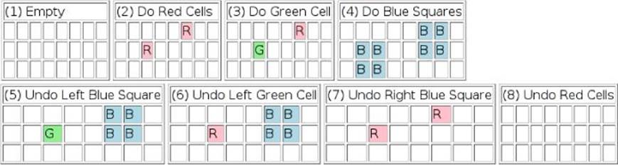
Figure 3.2 A grid being done and undone
class Grid:
def __init__(self, width, height):
self.__cells = [["white" for _ in range(height)]
for _ in range(width)]
def cell(self, x, y, color=None):
if color is None:
return self.__cells[x][y]
self.__cells[x][y] = color
@property
def rows(self):
return len(self.__cells[0])
@property
def columns(self):
return len(self.__cells)
This Grid class is a simple image-like class that holds a list of lists of color names.
The cell() method serves as both a getter (when the color argument is None) and a setter (when a color is given). The rows and columns read-only properties return the grid’s dimensions.
class UndoableGrid(Grid):
def create_cell_command(self, x, y, color):
def undo():
self.cell(x, y, undo.color)
def do():
undo.color = self.cell(x, y) # Subtle!
self.cell(x, y, color)
return Command.Command(do, undo, "Cell")
To make the Grid support undoable commands, we have created a subclass that adds two additional methods, the first of which is shown here.
Every command must be of type Command.Command or Command.Macro. The former takes do and undo callables and an optional description. The latter has an optional description and can have any number of Command.Commands added to it.
In the create_cell_command() method, we accept the position and color of the cell to set and then create the two functions required to create a Command.Command. Both commands simply set the given cell’s color.
Of course, at the time the do() and undo() functions are created, we cannot know what the color of the cell will be immediately before the do() command is applied, so we don’t know what color to undo it to. We have solved this problem by retrieving the cell’s color inside the do()function—at the time the function is called—and setting it as an attribute of the undo() function. Only then do we set the new color. Note that this works because the do() function is a closure that not only captures the x, y, and color parameters as part of its state, but also the undo()function that has just been created.
Once the do() and undo() functions have been created, we create a new Command.Command that incorporates them, plus a simple description, and return the command to the caller.
def create_rectangle_macro(self, x0, y0, x1, y1, color):
macro = Command.Macro("Rectangle")
for x in range(x0, x1 + 1):
for y in range(y0, y1 + 1):
macro.add(self.create_cell_command(x, y, color))
return macro
This is the second UndoableGrid method for creating doable–undoable commands. This method creates a macro that will create a rectangle spanning the given coordinates. For each cell to be colored, a cell command is created using the class’s other method (create_cell_command()), and this command is added to the macro. Once all the commands have been added, the macro is returned.
As we will see, both commands and macros support do() and undo() methods. Since commands and macros support the same methods, and macros contain commands, their relationship to each other is a variation of the Composite Pattern (§2.3, 40 ![]() ).
).
class Command:
def __init__(self, do, undo, description=""):
assert callable(do) and callable(undo)
self.do = do
self.undo = undo
self.description = description
def __call__(self):
self.do()
A Command.Command expects two callables: the first is the “do” command, and the second is the “undo” command. (The callable() function is a Python 3.3 built-in; for earlier versions an equivalent function can be created with: def callable(function): return isinstance(function, collections.Callable).)
A Command.Command can be executed simply by calling it (thanks to our implementation of the __call__() special method) or equivalently by calling its do() method. The command can be undone by calling its undo() method.
class Macro:
def __init__(self, description=""):
self.description = description
self.__commands = []
def add(self, command):
if not isinstance(command, Command):
raise TypeError("Expected object of type Command, got {}".
format(type(command).__name__))
self.__commands.append(command)
def __call__(self):
for command in self.__commands:
command()
do = __call__
def undo(self):
for command in reversed(self.__commands):
command.undo()
The Command.Macro class is used to encapsulate a sequence of commands that should all be done—or undone—as a single operation.* The Command.Macro offers the same interface as Command.Commands: do() and undo() methods, and the ability to be called directly. In addition, macros provide an add() method through which Command.Commands can be added.
*Although we speak of macros executing in a single operation, this operation is not atomic from a concurrency point of view, although it could be made atomic if we used appropriate locks.
For macros, commands must be undone in reverse order. For example, suppose we created a macro and added the commands A, B, and C. When we executed the macro (i.e., called it or called its do() method), it would execute A, then B, and then C. So when we call undo(), we must execute the undo() methods for C, then B, and then A.
In Python, functions, bound methods, and other callables are first-class objects that can be passed around and stored in data structures such as lists and dicts. This makes Python an ideal language for implementations of the Command Pattern. And the pattern itself can be used to great effect, as we have seen here, in providing do–undo functionality, as well as being able to support macros and deferred execution.
3.3. Interpreter Pattern
The Interpreter Pattern formalizes two common requirements: providing some means by which users can enter nonstring values into applications, and allowing users to program applications.
At the most basic level, an application will receive strings from the user—or from other programs—that must be interpreted (and perhaps executed) appropriately. Suppose, for example, we receive a string from the user that is supposed to represent an integer. An easy—and unwise—way to get the integer’s value is like this: i = eval(userCount). This is dangerous, because although we hope the string is something innocent like "1234", it could be "os.system('rmdir /s /q C:\\\\')".
In general, if we are given a string that is supposed to represent the value of a specific data type, we can use Python to obtain the value directly and safely.
try:
count = int(userCount)
when = datetime.datetime.strptime(userDate, "%Y/%m/%d").date()
except ValueError as err:
print(err)
In this snippet, we get Python to safely try to parse two strings, one into an int and the other into a datetime.date.
Sometimes, of course, we need to go beyond interpreting single strings into values. For example, we might want to provide an application with a calculator facility or allow users to create their own code snippets to be applied to application data. One popular approach to these kinds of requirements is to create a DSL (Domain Specific Language). Such languages can be created with Python out of the box—for example, by writing a recursive descent parser. However, it is much simpler to use a third-party parsing library such as PLY (www.dabeaz.com/ply), PyParsing (pyparsing.wikispaces.com), or one of the many other libraries that are available.*
*Parsing, including using PLY and PyParsing, is introduced in this author’s book, Programming in Python 3, Second Edition; see the Selected Bibliography for details (![]() 287).
287).
If we are in an environment where we can trust our applications’ users, we can give them access to the Python interpreter itself. The IDLE IDE (Integrated Development Environment) that is included with Python does exactly this, although IDLE is smart enough to execute user code in a separate process, so that if it crashes IDLE isn’t affected.
3.3.1. Expression Evaluation with eval()
The built-in eval() function evaluates a single string as an expression (with access to any global or local context we give it) and returns the result. This is sufficient to build the simple calculator.py application that we will review in this subsection. Let’s begin by looking at some interaction.
$ ./calculator.py
Enter an expression (Ctrl+D to quit): 65
A=65
ANS=65
Enter an expression (Ctrl+D to quit): 72
A=65, B=72
ANS=72
Enter an expression (Ctrl+D to quit): hypotenuse(A, B)
name 'hypotenuse' is not defined
Enter an expression (Ctrl+D to quit): hypot(A, B)
A=65, B=72, C=97.0
ANS=97.0
Enter an expression (Ctrl+D to quit): ^D
The user entered two sides of a right-angled triangle and then used the math.hypot() function (after making a mistake) to calculate the hypotenuse. After each expression is entered, the calculator.py program prints the variables it has created so far (and that are accessible to the user) and the answer to the current expression. (We have indicated user-entered text using bold—with Enter or Return at the end of each line implied—and Ctrl+D with ^D.)
To make the calculator as convenient as possible, the result of each expression entered is stored in a variable, starting with A, then B, and so on, and restarting at A if Z is reached. Furthermore, we have imported all the math module’s functions and constants (e.g., hypot(), e, pi, sin(), etc.) into the calculator’s namespace so that the user can access them without qualifying them (e.g., cos() rather than math.cos()).
If the user enters a string that cannot be evaluated, the calculator prints an error message and then repeats the prompt, and all the existing context is kept intact.
def main():
quit = "Ctrl+Z,Enter" if sys.platform.startswith("win") else "Ctrl+D"
prompt = "Enter an expression ({} to quit): ".format(quit)
current = types.SimpleNamespace(letter="A")
globalContext = global_context()
localContext = collections.OrderedDict()
while True:
try:
expression = input(prompt)
if expression:
calculate(expression, globalContext, localContext, current)
except EOFError:
print()
break
We have used EOF (End Of File) to signify that the user has finished. This means that the calculator can be used in a shell pipeline, accepting input redirected from a file, as well as for interactive user input.
We need to keep track of the name of the current variable (A or B or ...) so that we can update it each time a calculation is done. However, we can’t simply pass it as a string, since strings are copied and cannot be changed. A poor solution is to use a global variable. A better and much more common solution is to create a one-item list; for example, current = ["A"]. This list can be passed as current and its string can be read or changed by accessing it as current[0].
For this example, we have taken a more modern approach and created a tiny namespace with a single attribute (letter) whose value is "A". We can freely pass the current simple namespace instance around, and since it has a letter attribute, we can read or change the attribute’s value using the nice current.letter syntax.
The types.SimpleNamespace class was introduced in Python 3.3. For earlier versions an equivalent effect can be achieved by writing current = type("_", (), dict(letter="A"))(). This creates a new class called _ with a single attribute called letter with an initial value of "A". The built-in type() function returns the type of an object if called with one argument, or creates a new class if given a class name, a tuple of base classes, and a dictionary of attributes. If we pass an empty tuple, the base class will be object. Since we don’t need the class but only an instance, having called type(), we immediately call the class itself—hence the extra parentheses—to return the instance of it that we assign to current.
Python can supply the current global context using the built-in globals() function; this returns a dict that we can modify (e.g., add to, as we saw earlier; 23 ![]() ). Python can also supply the local context using the built-in locals() function, although the dict returned by this function must not be modified.
). Python can also supply the local context using the built-in locals() function, although the dict returned by this function must not be modified.
We want to provide a global context supplemented with the math module’s constants and functions and an initially empty local context. Although the global context must be a dict, the local context can be supplied as a dict—or as any other mapping object. Here, we have chosen to use acollections.OrderedDict—an insertion-ordered dictionary—as the locals context.
Since the calculator can be used interactively, we have created an event loop that is terminated when EOF is encountered. Inside the loop we prompt the user for input (also telling them how to quit), and if they enter any text, we call our calculate() function to perform the calculation and to print the results.
import math
def global_context():
globalContext = globals().copy()
for name in dir(math):
if not name.startswith("_"):
globalContext[name] = getattr(math, name)
return globalContext
This helper function starts by creating a local (shallow-copied) dict of the program’s global modules, functions, and variables. Then it iterates over all the public constants and functions in the math module and, for each one, adds its unqualified name to the globalContext dict and sets its value to be the actual math module constant or function it refers to. So, for example, when the name is "factorial", this name is added as a key in the globalContext, and its value is set to be the (i.e., a reference to the) math.factorial() function. This is what allows the calculator’s users to use unqualified names.
A simpler approach would have been to do from math import * and then use globals() directly, with no need for the globalContext dict. Such an approach is probably okay for the math module, but the way we have done it here provides finer control that might be more appropriate for other modules.
def calculate(expression, globalContext, localContext, current):
try:
result = eval(expression, globalContext, localContext)
update(localContext, result, current)
print(", ".join(["{}={}".format(variable, value)
for variable, value in localContext.items()]))
print("ANS={}".format(result))
except Exception as err:
print(err)
This is the function where we ask Python to evaluate the string expression using the global and local context dictionaries that we have created. If the eval() succeeds, we update the local context with the result and print the variables and the result. And if an exception occurs, we safely print it. Since we used a collections.OrderedDict for the local context, the items() method returns the items in insertion order without the need for an explicit sort. (Had we used a plain dict we would have needed to write sorted(localContext.items()).)
Although it is usually poor practice to use the Exception catch-all exception, it seems reasonable in this case, because the user’s expression could raise any kind of exception at all.
def update(localContext, result, current):
localContext[current.letter] = result
current.letter = chr(ord(current.letter) + 1)
if current.letter > "Z": # We only support 26 variables
current.letter = "A"
This function assigns the result to the next variable in the cyclic sequence A ... Z A ... Z .... This means that after the user has entered 26 expressions, the result of the last one is set as Z’s value, and the result of the next one will overwrite A’s value, and so on.
The eval() function will evaluate any Python expression. This is potentially dangerous if the expression is received from an untrusted source. An alternative is to use the standard library’s more restrictive—and safe—ast.literal_eval() function.
3.3.2. Code Evaluation with exec()
The built-in exec() function can be used to execute arbitrary pieces of Python code. Unlike eval(), exec() is not restricted to a single expression and always returns None. Context can be passed to exec() in the same way as for eval(), via globals and locals dictionaries. Results can be retrieved from exec() through the local context it is passed.
In this subsection, we will review the genome1.py program. This program creates a genome variable (a string of random A, C, G, and T letters) and executes eight pieces of user code with the genome in the code’s context.
context = dict(genome=genome, target="G[AC]{2}TT", replace="TCGA")
execute(code, context)
This code snippet shows the creation of the context dictionary with some data for the user’s code to work on and the execution of a user’s Code object (code) with the given context.
TRANSFORM, SUMMARIZE = ("TRANSFORM", "SUMMARIZE")
Code = collections.namedtuple("Code", "name code kind")
We expect user code to be provided in the form of Code named tuples, with a descriptive name, the code itself (as a string), and a kind—either TRANSFORM or SUMMARIZE. When executed, the user code should create either a result object or an error object. If their code’s kind isTRANSFORM, the result is expected to be a new genome string, and if the kind is SUMMARIZE, result is expected to be a number. Naturally, we will try to make our code robust enough to cope with user code that doesn’t meet these requirements.
def execute(code, context):
try:
exec(code.code, globals(), context)
result = context.get("result")
error = context.get("error")
handle_result(code, result, error)
except Exception as err:
print("'{}' raised an exception: {}\n".format(code.name, err))
This function performs the exec() call on the user’s code, using the program’s own global context and the provided local context. It then tries to retrieve the result and error objects, one of which the user code should have created, and passes them on to the customhandle_result() function.
Just as with the previous subsection’s eval() example, we have used the (normally to be avoided) Exception exception, since the user code could raise any kind of exception.
def handle_result(code, result, error):
if error is not None:
print("'{}' error: {}".format(code.name, error))
elif result is None:
print("'{}' produced no result".format(code.name))
elif code.kind == TRANSFORM:
genome = result
try:
print("'{}' produced a genome of length {}".format(code.name,
len(genome)))
except TypeError as err:
print("'{}' error: expected a sequence result: {}".format(
code.name, err))
elif code.kind == SUMMARIZE:
print("'{}' produced a result of {}".format(code.name, result))
print()
If the error object is not None, it is printed. Otherwise, if the result is None, we print a “produced no result” message. If we have a result and the user code’s kind is TRANSFORM, we assign result to genome, and in this case we simply print the genome’s new length. The try... except block is designed to protect our program from a user code error (e.g., returning a single value rather than a string or other sequence for a TRANSFORM). If the result’s kind is SUMMARIZE, we just print a summary line containing the result.
The genome1.py program has eight Code items: the first two (which we will see shortly) produce legitimate results, the third has a syntax error, the fourth reports an error, the fifth does nothing, the sixth has the wrong kind set, the seventh calls sys.exit(), and the eighth is never reached because the seventh terminates the program. Here is the program’s output.
$ ./genome1.py
'Count' produced a result of 12
'Replace' produced a genome of length 2394
'Exception Test' raised an exception: invalid syntax (<string>, line 4)
'Error Test' error: 'G[AC]{2}TT' not found
'No Result Test' produced no result
'Wrong Kind Test' error: expected a sequence result: object of type 'int' has
no len()
As the output makes clear, because the user code is executing in the same interpreter as the program itself, the user code can terminate or crash the program. (Note that the last line has been wrapped to fit on the page.)
Code("Count",
"""
import re
matches = re.findall(target, genome)
if matches:
result = len(matches)
else:
error = "'{}' not found".format(target)
""", SUMMARIZE)
This is the “Count” Code item. The item’s code does much more than is possible in a single expression of the kind that eval() could handle. The target and genome strings are taken from the context object that is passed as the exec()’s local context—and it is this same contextobject that any new variables (such as result and error) are implicitly stored in.
Code("Replace",
"""
import re
result, count = re.subn(target, replace, genome)
if not count:
error = "no '{}' replacements made".format(target)
""", TRANSFORM)
The “Replace” Code item’s code performs a simple transformation on the genome string, replacing nonoverlapping substrings that match the target regex with the replace string.
The re.subn() function (and regex.subn() method) performs substitutions exactly the same as re.sub() (and regex.sub()). However, whereas the sub() function (and method) returns a string where all the replacements have been made, the subn() function (and method) returns both the string and a count of how many replacements were made.
Although the genome1.py program’s execute() and handle_result() functions are easy to use and understand, in one respect the program is fragile: if the user code crashes—or simply calls sys.exit()—our program will terminate. In the next subsection we will explore a solution to this problem.
3.3.3. Code Evaluation Using a Subprocess
One possible answer to executing user code without compromising our application is to execute it in a separate process. This subsection’s genome2.py and genome3.py programs show how we can execute a Python interpreter in a subprocess, feed the interpreter with a program to execute through its standard input, and retrieve its results by reading its standard output.
We have given the genome2.py and genome3.py programs exactly the same eight Code items as the genome1.py program. Here is genome2.py’s output (genome3.py’s is identical):
$ ./genome2.py
'Count' produced a result of 12
'Replace' produced a genome of length 2394
'Exception Test' has an error on line 3
if genome[i] = "A":
^
SyntaxError: invalid syntax
'Error Test' error: 'G[AC]{2}TT' not found
'No Result Test' produced no result
'Wrong Kind Test' error: expected a sequence result: object of type 'int' has
no len()
'Termination Test' produced no result
'Length' produced a result of 2406
Notice that even though the seventh Code item calls sys.exit(), the genome2.py program continues afterward, merely reporting “produced no result” for that piece of code, and then going on to execute the “Length” code. (The genome1.py program was terminated by thesys.exit() call, so its last line of output was “...error: expected a sequence...”.) Another point to note is that genome2.py produces much better error reporting (e.g., the “Exception Test” code’s syntax error).
context = dict(genome=genome, target="G[AC]{2}TT", replace="TCGA")
execute(code, context)
The creation of the context and the execution of the user’s code with the context is exactly the same as for the genome1.py program.
def execute(code, context):
module, offset = create_module(code.code, context)
with subprocess.Popen([sys.executable, "-"], stdin=subprocess.PIPE,
stdout=subprocess.PIPE, stderr=subprocess.PIPE) as process:
communicate(process, code, module, offset)
This function begins by creating a string of code (module) containing the user’s code plus some supporting code that we will see in a moment. The offset is the number of lines we have added before the user’s code—this will help us to provide accurate line numbers in error messages. The function then starts a subprocess in which it executes a new instance of the Python interpreter, whose name is in sys.executable, and whose - (hyphen) argument means that the interpreter will expect to execute Python code sent to its sys.stdin.* The interaction with the process—including sending it the module code—is handled by our custom communicate() function.
*The subprocess.Popen() function added support for context managers (i.e., the with statement) in Python 3.2.
def create_module(code, context):
lines = ["import json", "result = error = None"]
for key, value in context.items():
lines.append("{} = {!r}".format(key, value))
offset = len(lines) + 1
outputLine = "\nprint(json.dumps((result, error)))"
return "\n".join(lines) + "\n" + code + outputLine, offset
This function creates a list of lines that will form a new Python module to be executed by a Python interpreter in a subprocess. The first line imports the json module that we will use to return results to the initiating process (i.e., to the genome2.py program). The second line initializes theresult and error variables to ensure that they exist. Then, we add a line for each of the context variables. Finally, we store the result and error (which the user’s code might have changed) inside a string using JSON (JavaScript Object Notation) that will be printed to sys.stdoutafter the user’s code has been executed.
UTF8 = "utf-8"
def communicate(process, code, module, offset):
stdout, stderr = process.communicate(module.encode(UTF8))
if stderr:
stderr = stderr.decode(UTF8).lstrip().replace(", in <module>", ":")
stderr = re.sub(", line (\d+)",
lambda match: str(int(match.group(1)) - offset), stderr)
print(re.sub(r'File."[^"]+?"', "'{}' has an error on line "
.format(code.name), stderr))
return
if stdout:
result, error = json.loads(stdout.decode(UTF8))
handle_result(code, result, error)
return
print("'{}' produced no result\n".format(code.name))
The communicate() function begins by sending the module code we created earlier to the subprocess’s Python interpreter to execute, and then blocks waiting for results to be produced. Once the interpreter finishes execution, its standard output and standard error output are collected in our local stdout and stderr variables. Note that all communication takes place using raw bytes—hence our need to encode the module string into UTF-8-encoded bytes.
If there is any error output (i.e., if an exception was raised, or if anything is written to sys.stderr), we replace the reported line number (which includes the lines we added before the user’s code) with the actual line number in the user’s code, and we replace the “File "<stdin>"” text with the Code object’s name. Then, we print the error text as a string.
The re.sub() call matches—and captures—the line number’s digits with (\d+) and replaces them with the result of the call to the lambda function given as its second argument. (More commonly, we give a string as second argument, but here we need to do some computation.) Thelambda function converts the digits into an integer and subtracts the offset, then returns the new line number as a string to replace the original. This ensures that the error message’s line number is correct for the user’s code, regardless of how many lines we put in front of it when creating the module we sent to be interpreted.
If there was no error output, but there was standard output, we decode the output’s bytes into a string (which we expect to be in JSON format) and parse this into Python objects—in this case a 2-tuple of a result and an error. Then we call our custom handle_result() function. (This function is identical in genome1.py, genome2.py, and genome3.py, and was shown earlier; 89 ![]() .)
.)
The genome2.py program’s user code is identical to genome1.py’s, although for genome2.py we provide some additional supporting code before and after the user code. Using JSON format to return results is safe and convenient but limits the data types we can return (e.g., result’s type) to dict, list, str, int, float, bool, or None, and where a dict or list may only contain objects of these types.
The genome3.py program is almost the same as genome2.py but returns its results in a pickle. This means that most Python types can be used.
def create_module(code, context):
lines = ["import pickle", "import sys", "result = error = None"]
for key, value in context.items():
lines.append("{} = {!r}".format(key, value))
offset = len(lines) + 1
outputLine = "\nsys.stdout.buffer.write(pickle.dumps((result, error)))"
return "\n".join(lines) + "\n" + code + outputLine, offset
This function is very similar to the genome2.py version. A minor difference is that we must import sys. The major difference is that whereas the json module’s loads() and dumps() methods work on strs, the pickle module’s equivalent functions work on bytes. So, here, we must write the raw bytes directly to sys.stdout’s underlying buffer to avoid the bytes being erroneously encoded.
def communicate(process, code, module, offset):
stdout, stderr = process.communicate(module.encode(UTF8))
...
if stdout:
result, error = pickle.loads(stdout)
handle_result(code, result, error)
return
The genome3.py program’s communicate() method is the same as for genome2.py (93 ![]() ) except for the line that has the loads() method call. For the JSON data we had to decode the bytes into a UTF-8-encoded str, but here we work directly on the raw bytes.
) except for the line that has the loads() method call. For the JSON data we had to decode the bytes into a UTF-8-encoded str, but here we work directly on the raw bytes.
Using exec() to execute arbitrary pieces of Python code received from the user or from other programs gives that code access to the full power of the Python interpreter—and to its entire standard library. And by executing the user code in a separate Python interpreter in a subprocess, we can protect our program from being crashed or terminated by it. However, we cannot really stop the user code from doing anything malicious. To execute untrusted code we would need to use some kind of sandbox; for example, the one provided by the PyPy Python interpreter (pypy.org).
For some programs, blocking while waiting for user code to finish execution might be acceptable, but it does run the risk of waiting “forever” if the user code has a bug (e.g., an infinite loop). One possible solution would be to create the subprocess in a separate thread and use a timer in the main thread. If the timer times out, we could then forcibly terminate the subprocess and report the problem to the user. Concurrent programming is introduced in the next chapter.
3.4. Iterator Pattern
The Iterator Pattern provides a way of sequentially accessing the items inside a collection or an aggregate object without exposing any of the internals of the collection or aggregate’s implementation. This pattern is so useful that Python provides built-in support for it, as well as providing special methods that we can implement in our own classes to make them seamlessly support iteration.
Iteration can be supported by satisfying the sequence protocol, or by using the two-argument form of the built-in iter() function, or by satisfying the iterator protocol. We will see examples of all these in the following subsections.
3.4.1. Sequence Protocol Iterators
One way to provide iterator support for our own classes is to make them support the sequence protocol. This means that we must implement a __getitem__() special method that can accept an integer index argument that starts from 0 and that raises an IndexError exception if no further iteration is possible.
for letter in AtoZ():
print(letter, end="")
print()
for letter in iter(AtoZ()):
print(letter, end="")
print()
ABCDEFGHIJKLMNOPQRSTUVWXYZ
ABCDEFGHIJKLMNOPQRSTUVWXYZ
These two code snippets create an AtoZ() object and then iterate over it. The object first returns the single character string "A", then "B", and so on, up to "Z". The object could have been made iterable in a number of ways, although in this case we’ve provided a __getitem__()method, as we will see in a moment.
In the second loop we have used the built-in iter() function to obtain an iterator to an instance of the AtoZ class. Clearly, this isn’t necessary in this case, but as we will see in a moment (and elsewhere in the book), iter() does have its uses.
class AtoZ:
def __getitem__(self, index):
if 0 <= index < 26:
return chr(index + ord("A"))
raise IndexError()
This is the complete AtoZ class. We have provided it with a __getitem__() method that satisfies the sequence protocol. When an object of this class is iterated, on the twenty-seventh iteration it will raise an IndexError. If this occurs inside a for loop, the exception is discarded, the loop is cleanly terminated, and execution resumes from the first statement after the loop.
3.4.2. Two-Argument iter() Function Iterators
Another way to provide iteration support is to use the built-in iter() function, but passing it two arguments instead of one. When this form is used, the first argument must be a callable (a function, a bound method, or any other callable object), and the second argument must be a sentinel value. When this form is used the callable is called at each iteration—with no arguments—and iteration will stop only if the callable raises a StopIteration exception or if it returns the sentinel value.
for president in iter(Presidents("George Bush"), None):
print(president, end=" * ")
print()
for president in iter(Presidents("George Bush"), "George W. Bush"):
print(president, end=" * ")
print()
George Bush * Bill Clinton * George W. Bush * Barack Obama *
George Bush * Bill Clinton *
The Presidents() call creates an instance of the Presidents class, and—thanks to the implementation of the __call__() special method—such instances are callable. So, here, we create a Presidents object that is a callable (as required by the two-argument form of the built-initer() function), and we provide a sentinel of None. A sentinel must be provided, even if it is None, so that Python knows to use the two-argument iter() function rather than the one-argument version.
The Presidents constructor creates a callable that will return each president in turn, starting with George Washington or, optionally, from the president we give it. In this case we told it to start from George Bush. Here, the first time we iterate, we have used a sentinel of None to signify “go to the end”, which, at the time of this writing, is Barack Obama. The second time we iterate we have provided the name of a president as the sentinel; this means that the callable will output each president from the first up to the one before the sentinel.
class Presidents:
__names = ("George Washington", "John Adams", "Thomas Jefferson",
...
"Bill Clinton", "George W. Bush", "Barack Obama")
def __init__(self, first=None):
self.index = (-1 if first is None else
Presidents.__names.index(first) - 1)
def __call__(self):
self.index += 1
if self.index < len(Presidents.__names):
return Presidents.__names[self.index]
raise StopIteration()
The Presidents class keeps a static (that is, class-wide) __names list with the names of all the U.S. presidents. The __init__() method sets the initial index to one less than either the first president in the list or the president the user has specified.
The instances of any class that implements the __call__() special method are callable. And when such an instance is called, it is this __call__() method that is actually executed.*
*In languages that don’t support functions as first-class objects, callable instances are called functors.
In this class’s __call__() special method, we either return the name of the next president in the list, or we raise a StopIteration exception. In the first iteration where the sentinel was None, the sentinel was never reached (since __call__() never returns None), but iteration still stopped cleanly because once we ran out of presidents, we raised the StopIteration exception. But in the second iteration, as soon as the sentinel president was returned to the built-in iter() function, the function itself raised StopIteration to terminate the loop.
3.4.3. Iterator Protocol Iterators
Probably the easiest way to provide iterator support in our own classes is to make them support the iterator protocol. This protocol requires that a class implements the __iter__() special method and that this method returns an iterator object. The iterator object must have its own__iter__() method that returns the iterator itself and a __next__() method that returns the next item—or that raises a StopIteration exception if there are no more items. Python’s for loop and in statement make use of this protocol under the hood. One simple way to implement an __iter__() method is to make it a generator—or to make it return a generator, since generators satisfy the iterator protocol. (See §3.1.2, 76 ![]() for more about generators.)
for more about generators.)
In this subsection we will create a simple bag class (also called a multiset). A bag is a collection class that is like a set but which allows duplicate items. An example bag is illustrated in Figure 3.3. Naturally, we will make the bag iterable and show three ways to do so. All the code is quoted from Bag1.py except where stated otherwise.
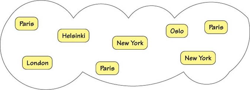
Figure 3.3 A bag is an unsorted collection of values with duplicates allowed
class Bag:
def __init__(self, items=None):
self.__bag = {}
if items is not None:
for item in items:
self.add(item)
The bag’s data is stored in the private self.__bag dictionary. The dictionary’s keys are anything hashable (i.e., they are the bag’s items), and the values are counts (i.e., how many of the item are in the bag). Users can add some initial items to a newly created bag if they wish.
def add(self, item):
self.__bag[item] = self.__bag.get(item, 0) + 1
Since self.__bag is not a collections.defaultdict, we must be careful to only increment an item that already exists; otherwise, we would get a KeyError exception. We use the dict.get() method to retrieve an existing item’s count, or 0 if there isn’t such an item, and set the dictionary to have an item with this number plus 1, creating the item if necessary.
def __delitem__(self, item):
if self.__bag.get(item) is not None:
self.__bag[item] -= 1
if self.__bag[item] <= 0:
del self.__bag[item]
else:
raise KeyError(str(item))
If an attempt is made to delete an item that isn’t in the bag, we raise a KeyError exception containing the item in string form. On the other hand, if the item is in the bag, we begin by reducing its count. If this drops to zero or less, we delete it from the bag.
We have not implemented the __getitem__() or __setitem__() special methods, because neither of them make sense for bags (since bags are unordered). Instead, we use bag.add() to add items, del bag[item] to delete items, and bag.count(item) to check how many of a particular item are in the bag.
def count(self, item):
return self.__bag.get(item, 0)
This method simply returns how many occurrences of the given item are in the bag—or zero if the item isn’t in the bag. A perfectly reasonable alternative would be to raise a KeyError for attempts to count an item that isn’t in the bag. This could be done simply by changing the method’s body to return self.__bag[item].
def __len__(self):
return sum(count for count in self.__bag.values())
This method is subtle since we must count all the duplicate items in the bag separately. To do this, we iterate over all the bag’s values (i.e., its item counts) and sum them using the built-in sum() function.
def __contains__(self, item):
return item in self.__bag
This method returns True if the bag contains at least one of the given item (since if an item is in the bag at all, its count is at least 1); otherwise, it returns False.
We have now seen all of the bag’s methods except for its iteration support. First, we’ll look at the Bag1.py module’s Bag.__iter__() method.
def __iter__(self): # This needlessly creates a list of items!
items = []
for item, count in self.__bag.items():
for _ in range(count):
items.append(item)
return iter(items)
This method is a first attempt. It builds up a list of items—as many of each as its count indicates—and then returns an iterator for the list. For a large bag, this could result in the creation of a very large list, which is rather inefficient, so we will look at two better approaches.
def __iter__(self):
for item, count in self.__bag.items():
for _ in range(count):
yield item
This code is from the Bag2.py module and is the only method that is different from Bag1.py’s Bag class.
Here, we iterate over the bag’s items, retrieving each item and its count, and yielding each item count times. There is a tiny fixed overhead for making the method a generator, but this is independent of the number of items, and of course, no separate list needs to be created, so this method is much more efficient than the Bag1.py version.
def __iter__(self):
return (item for item, count in self.__bag.items()
for _ in range(count))
Here is the Bag3.py module’s version of the Bag.__iter__() method. It is effectively the same as the Bag2.py module’s version, only instead of making the method into a generator, it returns a generator expression.
Although the book’s bag implementations work perfectly well, keep in mind that the standard library has its own bag implementation: collections.Counter.
3.5. Mediator Pattern
The Mediator Pattern provides a means of creating an object—the mediator—that can encapsulate the interactions between other objects. This makes it possible to achieve interactions between objects that have no direct knowledge of each other. For example, if a button object is clicked, it need only tell the mediator; then, it is up to the mediator to notify any objects that are interested in the button click. A mediator for a form with some text and button widgets, and a couple of associated methods, is illustrated in Figure 3.4.
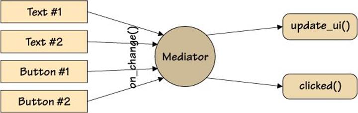
Figure 3.4 A form’s widget mediator
This pattern is clearly of great utility in GUI programming. In fact, all of the GUI toolkits available for Python (e.g., Tkinter, PyQt/PySide, PyGObject, wxPython) provide some equivalent facility. We will see Tkinter examples of this in Chapter 7 (![]() 231).
231).
In this section’s two subsections, we will look at two approaches to implementing a mediator. The first is quite conventional; the second uses coroutines. Both make use of Form, Button, and Text classes (whose implementations we will see) for a fictitious user interface toolkit.
3.5.1. A Conventional Mediator
In this subsection we will create a conventional mediator—a class that will orchestrate interactions—in this case, for a form. All the code shown here is from the mediator1.py program.
class Form:
def __init__(self):
self.create_widgets()
self.create_mediator()
Like most functions and methods shown in this book, this method has been ruthlessly refactored, in this case to the point where it passes on all its work.
def create_widgets(self):
self.nameText = Text()
self.emailText = Text()
self.okButton = Button("OK")
self.cancelButton = Button("Cancel")
This form has two text entry widgets for a user’s name and email address, and two buttons, OK and Cancel. Naturally, in a real user interface we would have to include label widgets, and then lay out the widgets, but here our example is purely to show the Mediator Pattern, so we don’t do any of that. We will see the Text and Button classes shortly.
def create_mediator(self):
self.mediator = Mediator(((self.nameText, self.update_ui),
(self.emailText, self.update_ui),
(self.okButton, self.clicked),
(self.cancelButton, self.clicked)))
self.update_ui()
We create a single mediator object for the entire form. This object takes one or more widget–callable pairs, which describe the relationships the mediator must support. In this case all the callables are bound methods. (See the “Bound and Unbound Methods” sidebar, 63 ![]() .) Here, we are saying that if the text of one of the text entry widgets changes, the Form.update_ui() method should be called; and that if one of the buttons is clicked, the Form.clicked() method should be called. After creating the mediator, we call the update_ui() method to initialize the form.
.) Here, we are saying that if the text of one of the text entry widgets changes, the Form.update_ui() method should be called; and that if one of the buttons is clicked, the Form.clicked() method should be called. After creating the mediator, we call the update_ui() method to initialize the form.
def update_ui(self, widget=None):
self.okButton.enabled = (bool(self.nameText.text) and
bool(self.emailText.text))
This method enables the OK button if both the text entry widgets have some text in them; otherwise it disables the button. Clearly, this method should be called whenever the text of one of the text entry widgets is changed.
def clicked(self, widget):
if widget == self.okButton:
print("OK")
elif widget == self.cancelButton:
print("Cancel")
This method is designed to be called whenever a button is clicked. In a real application it would do something more interesting than printing the button’s text.
class Mediator:
def __init__(self, widgetCallablePairs):
self.callablesForWidget = collections.defaultdict(list)
for widget, caller in widgetCallablePairs:
self.callablesForWidget[widget].append(caller)
widget.mediator = self
This is the first of the Mediator class’s two methods. We want to create a dictionary whose keys are widgets and whose values are lists of one or more callables. This is achieved by using a default dictionary. When we access an item in a default dictionary, if the item is not present, it is created and added with the value being created by the callable given to the dictionary in the first place. In this case, we gave the dictionary a list object, which when called returns a new empty list. So, the first time a particular widget is looked up in the dictionary, a new item is inserted with the widget as the key and an empty list as the value, and we immediately append the caller to the list. And whenever a widget is looked up subsequently, the caller is appended to the item’s existing list. We also set the widget’s mediator attribute (creating it if necessary) to this mediator (self).
The method adds the bound methods in the order they appear in the pairs; if we didn’t care about the order we could pass set instead of list when creating the default dictionary, and use set.add() instead of list.append() to add the bound methods.
def on_change(self, widget):
callables = self.callablesForWidget.get(widget)
if callables is not None:
for caller in callables:
caller(widget)
else:
raise AttributeError("No on_change() method registered for {}"
.format(widget))
Whenever a mediated object—that is, any widget passed to a Mediator—has a change of state, it is expected to call its mediator’s on_change() method. This method then retrieves and calls every bound method associated with the widget.
class Mediated:
def __init__(self):
self.mediator = None
def on_change(self):
if self.mediator is not None:
self.mediator.on_change(self)
This is a convenience class designed to be inherited by mediated classes. It keeps a reference to the mediator object, and if its on_change() method is called, it calls the mediator’s on_change() method, parameterized by this widget (i.e., self, the widget that has had a change of state).
Since this base class’s method is never modified in any of its subclasses, we could replace the base class with a class decorator, as we saw earlier (§2.4.2.2, 58 ![]() ).
).
class Button(Mediated):
def __init__(self, text=""):
super().__init__()
self.enabled = True
self.text = text
def click(self):
if self.enabled:
self.on_change()
This Button class inherits Mediated. This gives the button a self.mediator attribute and an on_change() method that it is expected to call when it experiences a change of state; for example, when it is clicked.
So, in this example, a call to Button.click() will result in a call to Button.on_change() (inherited from Mediated), which will result in a call to the media-tor’s on_change() method, which will then call whatever method or methods are associated with this button—in this case, the Form.clicked() method, with the button as the widget argument.
class Text(Mediated):
def __init__(self, text=""):
super().__init__()
self.__text = text
@property
def text(self):
return self.__text
@text.setter
def text(self, text):
if self.text != text:
self.__text = text
self.on_change()
Structurally, the Text class is the same as the Button class and also inherits Mediated.
For any widget (button, text entry, and so on), so long as we make them a Mediated subclass and call on_change() whenever they have a change of state, we can leave it to the Mediator to take care of the interactions. Of course, when we create the Mediator, we must also register the widgets and the associated methods we want called. This means that all of a form’s widgets are loosely coupled, thereby avoiding direct—and potentially fragile—relationships.
3.5.2. A Coroutine-Based Mediator
A mediator can be viewed as a pipeline that receives messages (on_change() calls) and passes these on to interested objects. As we have already seen (§3.1.2, 76 ![]() ), coroutines can be used to provide such facilities. All the code shown here is from the mediator2.py program, and all the code not shown is identical to that shown in the previous subsection from the mediator1.py program.
), coroutines can be used to provide such facilities. All the code shown here is from the mediator2.py program, and all the code not shown is identical to that shown in the previous subsection from the mediator1.py program.
The approach used in this subsection is different from that taken in the previous subsection. There, we associated pairs of widgets and methods, and whenever the widget notified it had changed, the mediator called the associated methods.
Here, every widget is given a mediator that is actually a pipeline of coroutines. Whenever a widget has a change of state, it sends itself into the pipeline, and it is up to the pipeline components (i.e., the coroutines) to decide whether they want to perform any action in response to a change in the widget they are sent.
def create_mediator(self):
self.mediator = self._update_ui_mediator(self._clicked_mediator())
for widget in (self.nameText, self.emailText, self.okButton,
self.cancelButton):
widget.mediator = self.mediator
self.mediator.send(None)
For the coroutine version we don’t need a separate mediator class. Instead, we create a pipeline of coroutines; in this case, one with two components, self._update_ui_mediator() and self._clicked_mediator(). (These are all Form methods.)
Once the pipeline is in place, we set each widget’s mediator attribute to the pipeline. And at the end, we send None down the pipeline. Since no widget is None, no widget-specific actions will be triggered, but any form-level actions (such as enabling or disabling the OK button in_update_ui_mediator()) will be performed.
@coroutine
def _update_ui_mediator(self, successor=None):
while True:
widget = (yield)
self.okButton.enabled = (bool(self.nameText.text) and
bool(self.emailText.text))
if successor is not None:
successor.send(widget)
This coroutine is part of the pipeline. (The @coroutine decorator was shown and discussed earlier; 77 ![]() .)
.)
Whenever a widget reports a change, the widget is passed into the pipeline and is returned by the yield expression into the widget variable. When it comes to enabling or disabling the OK button, we do this regardless of which widget has changed. (After all, it may be that no widget has changed, that widget is None, and so the form is simply being initialized.) After dealing with the button the coroutine passes on the changed widget to the next coroutine in the chain (if there is one).
@coroutine
def _clicked_mediator(self, successor=None):
while True:
widget = (yield)
if widget == self.okButton:
print("OK")
elif widget == self.cancelButton:
print("Cancel")
elif successor is not None:
successor.send(widget)
This pipeline coroutine is only concerned with OK and Cancel button clicks. If either of these buttons is the changed widget, this coroutine handles it; otherwise, it passes on the widget to the next coroutine, if any.
class Mediated:
def __init__(self):
self.mediator = None
def on_change(self):
if self.mediator is not None:
self.mediator.send(self)
The Button and Text classes are the same as for mediator1.py, but the Mediated class has one tiny change: if its on_change() method is called, it sends the changed widget (self) into the mediator pipeline.
As we mentioned in the previous subsection, the Mediated class could be replaced with a class decorator. The book’s examples include a mediator2d.py version of this example where this is done. (See §2.4.2.2, 58 ![]() .)
.)
The Mediator Pattern can also be varied to provide multiplexing; that is, many-to-many communications between objects. See, also, the Observer Pattern (§3.7, ![]() 107) and the State Pattern (§3.8,
107) and the State Pattern (§3.8, ![]() 111).
111).
3.6. Memento Pattern
The Memento Pattern is a means of saving and restoring an object’s state without violating encapsulation.
Python has support for this pattern out of the box: we can use the pickle module to pickle and unpickle arbitrary Python objects (with a few constraints; e.g., we cannot pickle a file object). In fact, Python can pickle None, bools, bytearrays, bytes, complexes, floats, ints, andstrs, as well as dicts, lists, and tuples that contain only pickleable objects (including collections), top-level functions, top-level classes, and instances of custom top-level classes whose __dict__ is pickleable; that is, objects of most custom classes. It is also possible to achieve the same effect using the json module, although this only supports Python’s basic types along with dictionaries and lists. (We saw examples of json and pickle use in §3.3.3, 91 ![]() ).
).
Even in the quite rare cases where we hit a limitation in what can be pickled, we can always add our own custom pickling support; for example, by implementing the __getstate__() and __setstate__() special methods, and possibly the __getnewargs__() method. Similarly, if we want to use JSON format with our own custom classes, we can extend the json module’s encoder and decoder.
We could also create our own format and protocols, but there is little point in doing so, given Python’s rich support for this pattern.
Unpickling essentially involves executing arbitrary Python code, so it is poor practice to unpickle pickles that are received from untrusted sources such as physical media or over a network connection. In such cases JSON is safer, or we can use checksums and encryption with pickling to ensure that the pickle hasn’t been meddled with.
3.7. Observer Pattern
The Observer Pattern supports many-to-many dependency relationships between objects, such that when one object changes state, all its related objects are notified. Nowadays, probably the most common expression of this pattern and its variants is the model/view/controller (MVC) paradigm. In this paradigm, a model represents data, one or more views visualize that data, and one or more controllers mediate between input (e.g., user interaction) and the model. And any changes to the model are automatically reflected in the associated views.
One popular simplification of the MVC approach is to use a model/view where the views both visualize the data and mediate input to the model; that is, the views and controllers are combined. In terms of the Observer Pattern, this means that the views are observers of the model, and the model is the subject being observed.
In this section we will create a model that represents a value with a minimum and a maximum (such as a scrollbar or slider widget or a temperature monitor). And we will create two separate observers (views) for the model: one to output the model’s value whenever it changes (as a kind of progress bar using HTML), and another to keep a history of the changes (their values and timestamps). Here is a sample run of the observer.py program.
$ ./observer.py > /tmp/observer.html
0 2013-04-09 14:12:01.043437
7 2013-04-09 14:12:01.043527
23 2013-04-09 14:12:01.043587
37 2013-04-09 14:12:01.043647
The history data is sent to sys.stderr and the HTML to sys.stdout, which we have redirected into an HTML file. The HTML page is shown in Figure 3.5. The program outputs four one-row HTML tables, the first when the (empty) model is first observed, and then each time the model is changed. Figure 3.6 illustrates the example’s model/view architecture.
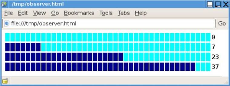
Figure 3.5 The observer example’s HTML output as the model changes
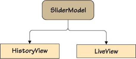
Figure 3.6 A model and two views
This section’s example, observer.py, uses an Observed base class to provide the functionality for adding, removing, and notifying observers. The SliderModel class provides a value with a minimum and maximum, and inherits the Observed class so that it can support being observed. And then we have two views that observe the model, HistoryView and LiveView. Naturally, we will review all of these classes, but first we will look at the program’s main() function to see how they are used and how the output shown earlier and in Figure 3.5 was obtained.
def main():
historyView = HistoryView()
liveView = LiveView()
model = SliderModel(0, 0, 40) # minimum, value, maximum
model.observers_add(historyView, liveView) # liveView produces output
for value in (7, 23, 37):
model.value = value # liveView produces output
for value, timestamp in historyView.data:
print("{:3} {}".format(value, datetime.datetime.fromtimestamp(
timestamp)), file=sys.stderr)
We begin by creating the two views. Next we create a model with a minimum of 0, a current value of 0, and a maximum of 40. Then we add the two views as observers of the model. As soon as the LiveView is added as an observer it produces its first output, and as soon as theHistoryView is added it records its first value and timestamp. We then update the model’s value three times, and at each update the LiveView outputs a new one-row HTML table and the HistoryView records the value and the timestamp.
At the end we print out the entire history to sys.stderr (i.e., to the console). The datetime.datetime.fromtimestamp() function accepts a timestamp (number of seconds since the epoch as returned by time.time()) and returns an equivalent datetime.datetimeobject. The str.format() method is smart enough to output datetime.datetimes in ISO-8601 format.
class Observed:
def __init__(self):
self.__observers = set()
def observers_add(self, observer, *observers):
for observer in itertools.chain((observer,), observers):
self.__observers.add(observer)
observer.update(self)
def observer_discard(self, observer):
self.__observers.discard(observer)
def observers_notify(self):
for observer in self.__observers:
observer.update(self)
This class is designed to be inherited by models or by any other class that wants to support observation. The Observed class maintains a set of observing objects. Whenever an object is added, its update() method is called to initialize it with the model’s current state. Then, whenever the model changes state it is expected to call its inherited observers_notify() method, so that every observer’s update() method can be called to ensure that every observer (i.e., every view) is representing the model’s new state.
The observers_add() method is subtle. We want to accept one or more observers to add, but using just *observers would allow zero or more. So, we require at least one observer (observer) and accept zero or more in addition (*observers). We could have done this using tuple concatenation (e.g., for observer in (observer,) + observers:), but we have used the more efficient itertools.chain() function instead. As noted earlier (46 ![]() ), this function accepts any number of iterables and returns a single iterable that is effectively the concatenation of all the iterables passed to it.
), this function accepts any number of iterables and returns a single iterable that is effectively the concatenation of all the iterables passed to it.
class SliderModel(Observed):
def __init__(self, minimum, value, maximum):
super().__init__()
# These must exist before using their property setters
self.__minimum = self.__value = self.__maximum = None
self.minimum = minimum
self.value = value
self.maximum = maximum
@property
def value(self):
return self.__value
@value.setter
def value(self, value):
if self.__value != value:
self.__value = value
self.observers_notify()
...
This is the particular model class for this example, but of course, it could be any kind of model. By inheriting Observed, the class gains a private set of observers (initially empty) and the observers_add(), observer_discard(), and observers_notify() methods. Whenever the model’s state changes—for example, when its value is changed—it must call its observers_notify() method so that any observers can respond accordingly.
The class also has minimum and maximum properties whose code has been elided; they are structurally identical to the value property, and, of course, their setters also call observers_notify().
class HistoryView:
def __init__(self):
self.data = []
def update(self, model):
self.data.append((model.value, time.time()))
This view is an observer of the model since it provides an update() method that accepts the observed model as its only argument besides self. Whenever the update() method is called, it adds a value–timestamp 2-tuple to its self.data list, thus preserving a history of all the changes that are applied to the model.
class LiveView:
def __init__(self, length=40):
self.length = length
This is another view that observes the model. The length is the number of cells used to represent the model’s value in a one-row HTML table.
def update(self, model):
tippingPoint = round(model.value * self.length /
(model.maximum - model.minimum))
td = '<td style="background-color: {}"> </td>'
html = ['<table style="font-family: monospace" border="0"><tr>']
html.extend(td.format("darkblue") * tippingPoint)
html.extend(td.format("cyan") * (self.length - tippingPoint))
html.append("<td>{}</td></tr></table>".format(model.value))
print("".join(html))
When the model is first observed, and whenever it is subsequently updated, this method is called. It outputs a one-row HTML table with self.length cells to represent the model, using cyan for empty cells and dark blue for filled cells. It determines how many of which kind of cell there are by calculating the tipping point between the filled cells (if there are any) and the empty cells.
The Observer Pattern is widely used in GUI programming and also has uses in the context of other event-processing architectures, such as simulations and servers. Examples include database triggers, Django’s signaling system, the Qt GUI application framework’s signals and slots mechanism, and many uses of WebSockets.
3.8. State Pattern
The State Pattern is intended to provide objects whose behavior changes when their state changes; that is, objects that have modes.
To illustrate this design pattern we will create a multiplexer class that has two states, and whose methods’ behavior changes depending on which state a multiplexer instance is in. When the multiplexer is in its active state, it can accept “connections”—that is, event name–callback pairs—where the callback is any Python callable (e.g., a lambda, a function, a bound method, etc.). After the connections have been made, whenever an event is sent to the multiplexer, the associated callbacks are called (providing the multiplexer is in its active state). If the multiplexer is dormant, calling its methods safely does nothing.
To show the multiplexer in use, we will create some callback functions that count the number of events they receive and connect them to an active multiplexer. Then we will send some random events to the multiplexer, and afterwards, print out the counts that the callbacks have accumulated. All the code is in the multi-plexer1.py program, and the program’s output for a sample run is shown here:
$ ./multiplexer1.py
After 100 active events: cars=150 vans=42 trucks=14 total=206
After 100 dormant events: cars=150 vans=42 trucks=14 total=206
After 100 active events: cars=303 vans=83 trucks=30 total=416
After sending the active multiplexer one-hundred random events, we change the multiplexer’s state to dormant, and then send it another hundred events—all of which should be ignored. Then we set the multiplexer back to its active state and send it more events; these it should respond to by calling the associated callbacks.
We will begin by looking at how the multiplexer is constructed, how the connections are made, and how events are sent. Then we will look at the callback functions and the event class. Finally, we will look at the multiplexer itself.
totalCounter = Counter()
carCounter = Counter("cars")
commercialCounter = Counter("vans", "trucks")
multiplexer = Multiplexer()
for eventName, callback in (("cars", carCounter),
("vans", commercialCounter), ("trucks", commercialCounter)):
multiplexer.connect(eventName, callback)
multiplexer.connect(eventName, totalCounter)
Here, we begin by creating some counters. Instances of these classes are callable, so they can be used wherever a function (e.g., a callback) is required. They maintain one independent count per name they are given, or if anonymous (like totalCounter) they maintain a single count.
Then we create a new multiplexer (which starts out active by default). Next, we connect callback functions to events. There are three event names we are interested in: “cars”, “vans”, and “trucks”. The carCounter() function is connected to the “cars” event; thecommercialCounter() function is connected to the “vans” and “trucks” events; and the totalCounter() function is connected to all three events.
for event in generate_random_events(100):
multiplexer.send(event)
print("After 100 active events: cars={} vans={} trucks={} total={}"
.format(carCounter.cars, commercialCounter.vans,
commercialCounter.trucks, totalCounter.count))
In this snippet, we generate one-hundred random events and send each one to the multiplexer. If, for example, an event is a “cars” event, the multiplexer will call the carCounter() and totalCounter() functions, passing the event as the sole argument for each call. Similarly, if the event is a “vans” or “trucks” event, both the commercialCounter() and totalCounter() functions are called.
class Counter:
def __init__(self, *names):
self.anonymous = not bool(names)
if self.anonymous:
self.count = 0
else:
for name in names:
if not name.isidentifier():
raise ValueError("names must be valid identifiers")
setattr(self, name, 0)
If no names are given, an instance of an anonymous counter is created whose count is kept in self.count. Otherwise, independent counts are created for the name or names passed in using the built-in setattr() function. For example, the carCounter instance is given aself.cars attribute, and the commercialCounter is given self.vans and self.trucks attributes.
def __call__(self, event):
if self.anonymous:
self.count += event.count
else:
count = getattr(self, event.name)
setattr(self, event.name, count + event.count)
When a Counter instance is called, the call is passed to this special method. If the counter is anonymous (e.g., totalCounter), the self.count is incremented. Otherwise, we try to retrieve the counter attribute corresponding to the event name. For example, if the event name is"trucks", we set count to be the value of self.trucks. Then we update the attribute’s value with the old count plus the new event count.
Since we haven’t provided a default value for the built-in getattr() function, if the attribute doesn’t exist (e.g., "truck"), the method will correctly raise an AttributeError. This also ensures that we don’t create a misnamed attribute by mistake since in such cases thesetattr() call is never reached.
class Event:
def __init__(self, name, count=1):
if not name.isidentifier():
raise ValueError("names must be valid identifiers")
self.name = name
self.count = count
This is the entire Event class. It is very simple since we just need it as part of the infrastructure for showing the State Pattern that’s exemplified by the Multiplexer class. Incidentally, the Multiplexer is also an example of the Observer Pattern (§3.7, 107 ![]() ).
).
3.8.1. Using State-Sensitive Methods
There are two main approaches that we can take to handling state within a class. One approach is to use state-sensitive methods, as we will see in this subsection. The other approach is to use state-specific methods, which we will cover in the next subsection (§3.8.2, ![]() 115).
115).
class Multiplexer:
ACTIVE, DORMANT = ("ACTIVE", "DORMANT")
def __init__(self):
self.callbacksForEvent = collections.defaultdict(list)
self.state = Multiplexer.ACTIVE
The Multiplexer class has two states (or modes): ACTIVE and DORMANT. When a Multiplexer instance is ACTIVE, its state-sensitive methods do useful work, but when it is DORMANT, its state-sensitive methods do nothing. We ensure that when a new Multiplexer is created, it starts off in the ACTIVE state.
The self.callbacksForEvent dictionary’s keys are event names and its values are lists of callables.
def connect(self, eventName, callback):
if self.state == Multiplexer.ACTIVE:
self.callbacksForEvent[eventName].append(callback)
This method is used to create an association between a named event and a callback. If the given event name isn’t already in the dictionary, the fact that self.callbacksForEvent is a default dictionary will ensure that an item with the event name as key is created with an empty list as its value, which it will then return. And if the event name is already in the dictionary, its list will be returned. So, in either case, we get a list that we can then append the new callback to. (We discussed default dictionaries earlier; 102 ![]() .)
.)
def disconnect(self, eventName, callback=None):
if self.state == Multiplexer.ACTIVE:
if callback is None:
del self.callbacksForEvent[eventName]
else:
self.callbacksForEvent[eventName].remove(callback)
If this method is called without specifying a callback, we interpret that to mean that the user wants to disconnect all the callbacks associated with the given event name. Otherwise, we remove only the specified callback from the given event name’s list of callbacks.
def send(self, event):
if self.state == Multiplexer.ACTIVE:
for callback in self.callbacksForEvent.get(event.name, ()):
callback(event)
If an event is sent to the multiplexer, and if the multiplexer is active, this method iterates over all the given event’s associated callbacks (of which there might not be any), and for each one, calls it with the event as argument.
3.8.2. Using State-Specific Methods
The multiplexer2.py program is almost the same as multiplexer1.py, only its Multiplexer class uses state-specific methods rather than the state-sensitive methods shown in the previous subsection. The Multiplexer class has the same two states and the same__init__() method as before. However, the self.state attribute is now a property.
@property
def state(self):
return (Multiplexer.ACTIVE if self.send == self.__active_send
else Multiplexer.DORMANT)
This version of the multiplexer doesn’t store the state as such. Instead, it computes the state by checking if one of the public methods has been set to an active or passive private method, as we’ll see next.
@state.setter
def state(self, state):
if state == Multiplexer.ACTIVE:
self.connect = self.__active_connect
self.disconnect = self.__active_disconnect
self.send = self.__active_send
else:
self.connect = lambda *args: None
self.disconnect = lambda *args: None
self.send = lambda *args: None
Whenever the state is changed, the state property’s setter sets the multiplexer to have a set of methods that are appropriate to the state. For example, if the state is set to be DORMANT, the anonymous lambda versions of the methods are assigned to the public methods.
def __active_connect(self, eventName, callback):
self.callbacksForEvent[eventName].append(callback)
Here, we have created a private active method: either this or an anonymous “do nothing” lambda method is assigned to the corresponding public method at any one time. We haven’t shown the private active disconnect or send methods, because they follow the same pattern. The key point to notice is that none of these methods checks the instance’s state (since they are only ever called in the appropriate state), which slightly simplifies them and makes them minutely faster.
Naturally, it is easy to do a coroutine-based version of the Multiplexer, but since we’ve already seen some coroutine examples, we won’t show another one here. (However, the examples’ multiplexer3.py program shows one approach to coroutine-based multiplexing.)
Although we have used the State Pattern for a multiplexer, having stateful (or modal) objects is quite common in a wide range of contexts.
3.9. Strategy Pattern
The Strategy Pattern provides a means of encapsulating a set of algorithms that can be used interchangeably, depending on the user’s needs.
For example, in this section we will create two different algorithms for arranging a list containing an arbitrary number of items in a table with a specified number of rows. One algorithm will produce a snippet of HTML output; Figure 3.7 shows the results for tables with two, three, and four rows. The other algorithm will produce plain text output, the results of which (for tables of four and five rows) are shown here:
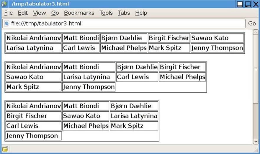
Figure 3.7 The tabulator program’s HTML table output
$ ./tabulator3.py
...
+-------------------+-------------------+-------------------+
| Nikolai Andrianov | Matt Biondi | Bjørn Dæhlie |
| Birgit Fischer | Sawao Kato | Larisa Latynina |
| Carl Lewis | Michael Phelps | Mark Spitz |
| Jenny Thompson | | |
+-------------------+-------------------+-------------------+
+-------------------+-------------------+
| Nikolai Andrianov | Matt Biondi |
| Bjørn Dæhlie | Birgit Fischer |
| Sawao Kato | Larisa Latynina |
| Carl Lewis | Michael Phelps |
| Mark Spitz | Jenny Thompson |
+-------------------+-------------------+
There are a number of approaches we could take to parameterizing by algorithm. One obvious approach is to create a Layout class that accepts a Tabulator instance, which performs the appropriate tabulated layout. The tabulator1.py program (not shown) takes this approach. A refinement, for tabulators that don’t need to maintain state, is to use static methods and to pass the tabulator class rather than an instance to provide the algorithm. The tabulator2.py program (again, not shown) does this.
In this section, we will show a simpler and even more refined technique: a Layout class that accepts a tabulation function that implements the desired algorithm.
WINNERS = ("Nikolai Andrianov", "Matt Biondi", "Bjørn Dæhlie",
"Birgit Fischer", "Sawao Kato", "Larisa Latynina", "Carl Lewis",
"Michael Phelps", "Mark Spitz", "Jenny Thompson")
def main():
htmlLayout = Layout(html_tabulator)
for rows in range(2, 6):
print(htmlLayout.tabulate(rows, WINNERS))
textLayout = Layout(text_tabulator)
for rows in range(2, 6):
print(textLayout.tabulate(rows, WINNERS))
In this function we create two Layout objects, each parameterized by a different tabulator function. For each layout we print a table with two rows, with three rows, with four rows, and with five rows.
class Layout:
def __init__(self, tabulator):
self.tabulator = tabulator
def tabulate(self, rows, items):
return self.tabulator(rows, items)
This class supports only one algorithm: tabulate. The function that implements the algorithm is expected to accept a row count and a sequence of items and to return the tabulated results.
In fact, we could reduce this class even more: here is the tabulator4.py version.
class Layout:
def __init__(self, tabulator):
self.tabulate = tabulator
Here, we have made the self.tabulate attribute a callable (the passed-in tabulator function). The calls shown in main() work exactly the same for tabulator3.py’s and tabulator4.py’s Layout classes.
Although the actual tabulation algorithms aren’t relevant to the design pattern itself, we will very briefly review one of them for the sake of completeness.
def html_tabulator(rows, items):
columns, remainder = divmod(len(items), rows)
if remainder:
columns += 1
column = 0
table = ['<table border="1">\n']
for item in items:
if column == 0:
table.append("<tr>")
table.append("<td>{}</td>".format(escape(str(item))))
column += 1
if column == columns:
table.append("</tr>\n")
column %= columns
if table[-1][-1] != "\n":
table.append("</tr>\n")
table.append("</table>\n")
return "".join(table)
For both tabulator functions, we must calculate the number of columns needed to put all the items in a table with the specified number of rows. Once we have this number (columns), we can iterate over all the items while keeping track of the current column in the current row.
The text_tabulator() function (not shown) is slightly longer but uses essentially the same approach.
In more realistic contexts we might use algorithms that are radically different—both in terms of their code and their performance characteristics—so as to allow users to choose the most appropriate trade-offs for their particular uses. Plugging in different algorithms as callables—lambdas, functions, bound methods—is straightforward because Python treats callables as first-class objects; that is, as objects that can be passed and stored in collections like any other kind of object.
3.10. Template Method Pattern
The Template Method Pattern allows us to define the steps of an algorithm but defer the execution of some of those steps to subclasses.
In this section we will create an AbstractWordCounter class that provides two methods. The first, can_count(filename), is expected to return a Boolean indicating whether the class can count the words in the given file (based on the file’s extension). The second, count(filename), is expected to return a word count. We will also create two subclasses: one for word-counting plain text files and the other for word-counting HTML files. Let’s start by seeing the classes in action (with the code taken from wordcount1.py):
def count_words(filename):
for wordCounter in (PlainTextWordCounter, HtmlWordCounter):
if wordCounter.can_count(filename):
return wordCounter.count(filename)
We have made all the methods in all the classes static. This means that no per-instance state can be maintained (because there are no instances as such) and that we can work directly on class objects rather than on instances. (It would be easy to make the methods nonstatic and use instances if we did need to maintain any state.)
Here, we iterate over our two word-counting subclasses’ class objects, and if one of them is able to count the words in the given file, we perform and return the count. If neither of them can, we (implicitly) return None to signify that we couldn’t do a count at all.
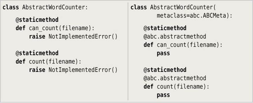
This purely abstract class provides the word-counter interface, whose methods subclasses must reimplement. The left-hand code snippet, from wordcount1.py, takes a more traditional approach. The right-hand code snippet, from word-count2.py, takes a more modern approach using the abc (abstract base class) module.
class PlainTextWordCounter(AbstractWordCounter):
@staticmethod
def can_count(filename):
return filename.lower().endswith(".txt")
@staticmethod
def count(filename):
if not PlainTextWordCounter.can_count(filename):
return 0
regex = re.compile(r"\w+")
total = 0
with open(filename, encoding="utf-8") as file:
for line in file:
for _ in regex.finditer(line):
total += 1
return total
This subclass implements the word-counter interface using a very simplistic notion of what constitutes a word, and assuming that all .txt files are encoded using UTF-8 (or 7-bit ASCII, since that’s a subset of UTF-8).
class HtmlWordCounter(AbstractWordCounter):
@staticmethod
def can_count(filename):
return filename.lower().endswith((".htm", ".html"))
@staticmethod
def count(filename):
if not HtmlWordCounter.can_count(filename):
return 0
parser = HtmlWordCounter.__HtmlParser()
with open(filename, encoding="utf-8") as file:
parser.feed(file.read())
return parser.count
This subclass provides the word-counter interface for HTML files. It uses its own private HTML parser (itself an html.parser.HTMLParser subclass embedded inside the HtmlWordCounter class, which we will see in a moment). With the private HTML parser in place, all we need to do to count the words in an HTML file is create an instance of the parser and give it the HTML to parse. Once parsing is complete, we return the word count that the parser has accumulated for us.
For completeness, we will review the embedded HtmlWordCounter.__HtmlParser that does the actual counting. The Python standard library’s HTML parser works rather like a SAX (Simple API for XML) parser, in that it iterates over the text and calls particular methods when corresponding events (i.e., “start tag”, “end tag”, etc.) occur. So, to make use of the parser we must subclass it and reimplement those methods that correspond to the events we are interested in.
class __HtmlParser(html.parser.HTMLParser):
def __init__(self):
super().__init__()
self.regex = re.compile(r"\w+")
self.inText = True
self.text = []
self.count = 0
We have made the embedded html.parser.HTMLParser subclass private and added four items of data to it. The self.regex holds our simple definition of a “word” (a sequence of one or more letters, digits, or underscores). The self.inText bool indicates whether text we encounter is a piece of a value such as user-visible text (as opposed to being inside a <script> or <style> tag). The self.text will hold the piece or pieces of text that make up the current value, and the self.count is the word count.
def handle_starttag(self, tag, attrs):
if tag in {"script", "style"}:
self.inText = False
This method’s name and signature (and that of all the handle_...() methods) is determined by the base class. By default, handler methods do nothing, so, naturally, we must reimplement any that we are interested in.
We do not want to count the words inside embedded scripts or style sheets, so if we encounter their start tags, we switch off text accumulation.
def handle_endtag(self, tag):
if tag in {"script", "style"}:
self.inText = True
else:
for _ in self.regex.finditer(" ".join(self.text)):
self.count += 1
self.text = []
If we reach the end of a script or style sheet tag, we switch text accumulation back on. In all other cases we iterate over the accumulated text and count the words. Then we reset the accumulated text to be an empty list.
def handle_data(self, text):
if self.inText:
text = text.rstrip()
if text:
self.text.append(text)
If we receive text and we are not inside a script or style sheet, we accumulate the text.
Thanks to the power and flexibility of Python’s support for private nested classes, and its library’s html.parser.HTMLParser, we can do fairly sophisticated parsing while hiding all the details from users of the HtmlWordCounter class.
The Template Method Pattern is in some ways similar to the Bridge Pattern we saw earlier (§2.2, 34 ![]() ).
).
3.11. Visitor Pattern
The Visitor Pattern is used to apply a function to every item in a collection or aggregate object. This is different from a typical use of the Iterator Pattern (§3.4, 95 ![]() )—where we would iterate over a collection or aggregate and call a method on each item—since with a “visitor”, we are applying an external function rather than calling a method.
)—where we would iterate over a collection or aggregate and call a method on each item—since with a “visitor”, we are applying an external function rather than calling a method.
Python has built-in support for this pattern. For example, newList = map(function, oldSequence) will call the function() on every item in the oldSequence to produce the newList. The same can be done using a list comprehension: newList = [function(item) for item inoldSequence].
If we need to apply a function to every item in a collection or aggregate object, then we can iterate over it using a for loop: for item in collection: function(item). If the items are of different types, we can use if statements and the built-in isinstance() function to distinguish between them to choose the type-appropriate code to execute inside the function().
Some of the behavioral patterns have direct support in the Python language; those that don’t are simple to implement. The Chain of Responsibility, Mediator, and Observer Patterns can all be implemented conventionally or using coroutines, and they all provide variations on the theme of decoupled inter-object communication. The Command Pattern can be used to provide lazy evaluation and do–undo facilities. Since Python is a (byte-code) interpreted language, we can implement the Interpreter Pattern using Python itself and can even isolate the interpreted code in a separate process. Support for the Iterator Pattern (and, implicitly, the Visitor Pattern) is built in to Python. The Memento Pattern is well supported by Python’s standard library (e.g., using the pickle or json modules). The State, Strategy, and Template Method Patterns have no direct support, but are all easy to implement.
Design patterns provide useful ways of thinking about, organizing, and implementing code. Some of the patterns are only applicable to the object-oriented programming paradigm, while others can be used for both procedural and object-oriented programming. Since the publication of the original design patterns book, there has been—and there continues to be—a great deal of research into the subject. The best starting point for learning more is the educational, not-forprofit Hillside Group’s web site (hillside.net).
In the next chapter, we will look at a different programming paradigm—concur-rency—to try to achieve improved performance by taking advantage of modern multi-core hardware. But before looking into concurrency, we will do our first case study, developing an image-handling package that we will use and refer to in various ways at several points throughout the book.
3.12. Case Study: An Image Package
The Python standard library does not include any image processing modules, as such. However, it is possible to create, load, and save images using Tkinter’s tk.PhotoImage class. (The barchart2.py example shows how this can be done.) Unfortunately, Tkinter can only read and write the unpopular GIF, PPM, and PGM image formats, although once Python comes with Tcl/Tk 8.6, the popular PNG format will be supported. Even so, the tk.PhotoImage class can only be used in a single thread (the main GUI thread), so it is of no use if we want to handle multiple images concurrently.
We could, of course, use a third-party image library like Pillow (github.com/python-imaging/Pillow) or use another GUI toolkit.* But we have decided to implement our own image package to provide this case study and to serve as the basis for another one later on.
*If we wanted to plot 2D data, we could use the third-party matplotlib package (matplotlib.org).
We want our image package to store its image data efficiently and to be able to work with Python out of the box. To this end, we will represent an image as a linear array of colors. Each color (i.e., each pixel) will be represented by an unsigned 32-bit integer whose four bytes represent the alpha (transparency), red, green, and blue color components; this is sometimes called ARGB format. Since we are using a one-dimensional array, the pixel at image coordinate x, y is in array element (y × width) + x. This is illustrated in Figure 3.8, where the highlighted pixel in an 8 × 8 image is at coordinate (5, 1); that is, index position 13 ((1 × 8) + 5) in the array.
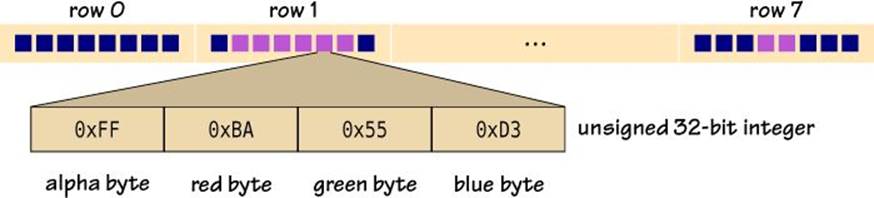
Figure 3.8 An array of Image color values for an 8 × 8 image
The Python standard library provides the array module for one-dimensional, type-specific arrays, and so is ideal for our purpose. However, the third-party numpy module offers highly optimized code for handling arrays (of any number of dimensions), so it would be good to take advantage of this module when it is available. Therefore, we will design the Image package to use numpy when possible, with array as a fallback. This means that Image will work in all cases but won’t be able to take as much advantage of numpy as possible, because the code must work interchangeably with both array.arrays and numpy.ndarrays.
We want to create and modify arbitrary images; however, we also want to be able to load existing images and to save created or modified images. Since loading and saving depends on the image format, we have designed the image package to have one module for handling images generically and separate modules (one per image format) for handling loading and saving. Furthermore, we will make the package capable of automatically taking advantage of any new image format modules that are added to the package—even after deployment—providing they meet the image package’s interface requirements.
The Image package consists of four modules. The Image/__init__.py module provides all the generic functionality. The other three modules provide format-specific loading and saving code. These are Image/Xbm.py for XBM (.xbm) format monochrome bitmaps,Image/Xpm.py for XPM (.xpm) format color pixmaps, and Image/Png.py for PNG (.png) format. The PNG format is very complicated, and there is already a Python module that supports it—PyPNG (github.com/drj11/pypng)—so our Png.py module will simply provide a thin wrapper (using the Adapter Pattern; §2.1, 29 ![]() ) around PyPNG, if it is available.
) around PyPNG, if it is available.
We will begin by looking at the generic image module (Image/__init__.py). Then we will review the Image/Xpm.py module, skipping the low-level details. Finally, we will look at the complete Image/Png.py wrapper module.
3.12.1. The Generic Image Module
The Image module provides the Image class plus a number of convenience functions and constants to support image processing.
try:
import numpy
except ImportError:
numpy = None
import array
One key issue is whether the image data is represented using an array.array or a numpy.ndarray, so after the normal imports, we try to import numpy. If the import fails, we fall back to importing the standard library’s array module to provide the necessary functionality, and create a numpy variable with value None for those few places where the difference between array and numpy matters.
We want our users to be able to access the image module with a simple import Image statement. And when they do this, we want all the available image-format–specific modules that provide load and save functions to be automatically available. This means that the user should be able to create and save a red 64 × 64 square using code like this:
import Image
image = Image.Image.create(64, 64, Image.color_for_name("red"))
image.save("red_64x64.xpm")
We want this to work even though the user hasn’t explicitly imported the Image/Xpm.py module. And, of course, we want this to work with any other image format modules that happen to be in the Image directory, even if they are added after the image package is initially deployed.
To support this functionality, we have included code in Image/__init__.py that automatically tries to load image format modules.
_Modules = []
for name in os.listdir(os.path.dirname(__file__)):
if not name.startswith("_") and name.endswith(".py"):
name = "." + os.path.splitext(name)[0]
try:
module = importlib.import_module(name, "Image")
_Modules.append(module)
except ImportError as err:
warnings.warn("failed to load Image module: {}".format(err))
del name, module
This code populates the private _Modules list with any modules that are found and imported from the Image directory, except for __init__.py (or any other module whose name begins with an underscore).
The code works by iterating over the files in the Image directory (wherever it happens to be in the file system). For each suitable .py file, we obtain the module name based on the filename. We must be careful to precede the module’s name with . since we want to import the module relative to the Image package. When using a relative import like this we must provide the package name as the importlib.import_module() function’s second argument. If the import succeeds, we add the corresponding Python module object to the list of modules; we’ll see how they are used shortly.
To avoid cluttering up the Image namespace, we have deleted the name and module variables once they are no longer needed.
The plugin approach used here is easy to use and understand and works well in most cases. However, it does suffer from a limitation: it won’t work if the Image package is put inside a .zip file. (Recall that Python can import modules that are inside .zip files: we just have to insert the.zip file into the sys.path list and then import as if the .zip file were a normal module; see docs.python. org/dev/library/zipimport.html.) A solution to this problem is to use the standard library’s pkgutil.walk_packages() function (instead ofos.listdir(), and adapting the code accordingly), since this function can work both with normal packages and with those inside .zip files; it can also cope with implementations provided as C extensions and precompiled byte code files (.pyc and .pyo).
class Image:
def __init__(self, width=None, height=None, filename=None,
background=None, pixels=None):
assert (width is not None and (height is not None or
pixels is not None) or (filename is not None))
if filename is not None: # From file
self.load(filename)
elif pixels is not None: # From data
self.width = width
self.height = len(pixels) // width
self.filename = filename
self.meta = {}
self.pixels = pixels
else: # Empty
self.width = width
self.height = height
self.filename = filename
self.meta = {}
self.pixels = create_array(width, height, background)
The image’s __init__() method has a rather complicated signature, but this doesn’t matter, because we will encourage our users to use much simpler convenience class methods to create images instead (for example, the Image.Image. create() method we saw earlier; 126 ![]() ).
).
@classmethod
def from_file(Class, filename):
return Class(filename=filename)
@classmethod
def create(Class, width, height, background=None):
return Class(width=width, height=height, background=background)
@classmethod
def from_data(Class, width, pixels):
return Class(width=width, pixels=pixels)
Here are the three image-creating factory class methods. These methods can be called on the class itself (e.g., image = Image.Image.create(200, 400)) and will work correctly for Image subclasses.
The from_file() method creates an image from a filename. The create() method creates an empty image with the given background color (or with a transparent background, if no color is specified). The from_data() method creates an image of the given width and with the pixels (i.e., colors) from the one-dimensional pixels array (of type array.array or numpy.ndarray).
def create_array(width, height, background=None):
if numpy is not None:
if background is None:
return numpy.zeros(width * height, dtype=numpy.uint32)
else:
iterable = (background for _ in range(width * height))
return numpy.fromiter(iterable, numpy.uint32)
else:
typecode = "I" if array.array("I").itemsize >= 4 else "L"
background = (background if background is not None else
ColorForName["transparent"])
return array.array(typecode, [background] * width * height)
This function creates a one-dimensional array of 32-bit unsigned integers (see Figure 3.8; 125 ![]() ). If numpy is present and the background is transparent, we can use the numpy.zeros() factory function to create the array with every integer set to zero (i.e., to 0x00000000). Any number with a zero alpha component is fully transparent. If a background color has been given, we create a generator expression that will produce width × height values (all of which are the same: background) and pass this iterator to the numpy.fromiter() factory function.
). If numpy is present and the background is transparent, we can use the numpy.zeros() factory function to create the array with every integer set to zero (i.e., to 0x00000000). Any number with a zero alpha component is fully transparent. If a background color has been given, we create a generator expression that will produce width × height values (all of which are the same: background) and pass this iterator to the numpy.fromiter() factory function.
If numpy is not available, we must create an array.array. Unlike numpy, this module does not allow us to specify the exact size of the integers we want it to hold, so we do the best we can. We use the "I" type specifier (unsigned integer, minimum size two bytes) if it is actually four or more bytes; otherwise, we use the "L" type specifier (unsigned integer, minimum size four bytes). This is to ensure that we use the smallest-sized integer that can hold four bytes, even on 64-bit machines where an unsigned integer would normally occupy eight bytes. We then create an array to hold items of the type specifier’s type and populate it with width × height background values. (We discuss the ColorForName default dictionary further on; ![]() 134.)
134.)
class Error(Exception): pass
This class provides us with an Image.Error exception type. We could have simply used one of the built-in exceptions (e.g., ValueError), but this makes it easier for Image users to catch image-specific exceptions without risking masking any other exceptions.
def load(self, filename):
module = Image._choose_module("can_load", filename)
if module is not None:
self.width = self.height = None
self.meta = {}
module.load(self, filename)
self.filename = filename
else:
raise Error("no Image module can load files of type {}".format(
os.path.splitext(filename)[1]))
The Image.__init__.py module has no knowledge of image file formats. However, the image-specific modules do have such knowledge, and they were loaded earlier when we populated the _Modules list (126 ![]() ). The image-specific modules could be considered variations of the Template Method Pattern (§3.10, 119
). The image-specific modules could be considered variations of the Template Method Pattern (§3.10, 119 ![]() ) or of the Strategy Pattern (§3.9, 116
) or of the Strategy Pattern (§3.9, 116 ![]() ).
).
Here, we try to retrieve a module that can load the given filename. If we get a suitable module, we initialize some of the image’s instance variables and tell the module to load the file. If the module’s load() method succeeds, it will populate self.pixels with an array of color values and set self.width and self.height appropriately; otherwise, it will raise an exception. (We’ll see examples of format-specific load() methods in subsections §3.12.2, ![]() 136, and §3.12.3,
136, and §3.12.3, ![]() 138.)
138.)
@staticmethod
def _choose_module(actionName, filename):
bestRating = 0
bestModule = None
for module in _Modules:
action = getattr(module, actionName, None)
if action is not None:
rating = action(filename)
if rating > bestRating:
bestRating = rating
bestModule = module
return bestModule
This static method is used to find a module in the private _Modules list that can perform the action (actionName) on the file (filename). It iterates over all the loaded modules and for each one tries to retrieve the actionName function (e.g., can_load() or can_save()) using the built-in getattr() function. For each action function found, the method calls the function with the given filename.
The action function is expected to return an integer of value 0 if it cannot perform the action at all, 100 if it can perform the action perfectly, or somewhere in between if it can perform the action imperfectly. For example, the Image/Xbm.py module returns 100 for files with the .xbmextension, since the module fully supports the format, but returns 0 for all other extensions. However, the Image/Xpm.py module returns only 80 for .xpm files, because it does not support the full XPM specification (although it works perfectly on all the .xpm files it has been tested on).
At the end, the module with the highest rating is returned, or if there is no suitable module None is returned.
def save(self, filename=None):
filename = filename if filename is not None else self.filename
if not filename:
raise Error("can't save without a filename")
module = Image._choose_module("can_save", filename)
if module is not None:
module.save(self, filename)
self.filename = filename
else:
raise Error("no Image module can save files of type {}".format(
os.path.splitext(filename)[1]))
This method is very similar to the load() method in that it tries to get a module that can save a file with the given filename (i.e., one that can save in the format indicated by the file’s extension) and performs the save.
def pixel(self, x, y):
return self.pixels[(y * self.width) + x]
The pixel() method returns the color at the given position as an ARGB value (i.e., an unsigned 32-bit integer).
def set_pixel(self, x, y, color):
self.pixels[(y * self.width) + x] = color
The set_pixel() method sets the given pixel to the given ARGB value if the x and y coordinates are in range; otherwise, it raises an IndexError exception.
The Image module provides some basic drawing methods including line(), ellipse(), and rectangle(). We will just show one representative method here.
def line(self, x0, y0, x1, y1, color):
Δx = abs(x1 - x0)
Δy = abs(y1 - y0)
xInc = 1 if x0 < x1 else -1
yInc = 1 if y0 < y1 else -1
δ = Δx - Δy
while True:
self.set_pixel(x0, y0, color)
if x0 == x1 and y0 == y1:
break
δ2 = 2 * δ
if δ2 > -Δy:
δ -= Δy
x0 += xInc
if δ2 < Δx:
δ += Δx
y0 += yInc
This method uses Bresenham’s line algorithm (which requires only integer arithmetic) to draw a line from point (x0, y0) to point (x1, y1).* Thanks to Python 3’s Unicode support, we are able to use variable names that are natural for this context; for example, Δx and Δy to represent differences in x and y coordinate values, and Δ and Δ2 for the error values.
*This algorithm is explained at en.wikipedia.org/wiki/Bresenham's_line_algorithm.
def scale(self, ratio):
assert 0 < ratio < 1
rows = round(self.height * ratio)
columns = round(self.width * ratio)
pixels = create_array(columns, rows)
yStep = self.height / rows
xStep = self.width / columns
index = 0
for row in range(rows):
y0 = round(row * yStep)
y1 = round(y0 + yStep)
for column in range(columns):
x0 = round(column * xStep)
x1 = round(x0 + xStep)
pixels[index] = self._mean(x0, y0, x1, y1)
index += 1
return self.from_data(columns, pixels)
This method creates and returns a new image that is a scaled-down version of this image. The ratio should be in the interval (0.0, 1.0), with a ratio of 0.75 producing an image with its width and height ¾ their original sizes, and a ratio of 0.5 producing an image ¼ of the original size, that is, with half the width and height. Each pixel (i.e., each color) in the resultant image is the average (mean) of the colors in the rectangle of the source image that the pixel must represent.
The image’s x, y coordinates are integers, but to avoid inaccuracies we must use floating-point arithmetic (e.g., using / rather than //) as we step through the pixel data. So, we use the built-in round() function whenever we need integers. And at the end, we use theImage.Image.from_data() convenience factory class method to create a new image based on the computed number of columns and using the pixels array we have created and populated with colors.
def _mean(self, x0, y0, x1, y1):
αTotal, redTotal, greenTotal, blueTotal, count = 0, 0, 0, 0, 0
for y in range(y0, y1):
if y >= self.height:
break
offset = y * self.width
for x in range(x0, x1):
if x >= self.width:
break
α, r, g, b = self.argb_for_color(self.pixels[offset + x])
αTotal += α
redTotal += r
greenTotal += g
blueTotal += b
count += 1
α = round(αTotal / count)
r = round(redTotal / count)
g = round(greenTotal / count)
b = round(blueTotal / count)
return self.color_for_argb(α, r, g, b)
This private method accumulates the sums of the alpha, red, green, and blue components of all the pixels in the rectangle specified by the x0, y0, x1, y1 coordinates. Each of these sums is then divided by the number of pixels that were examined to produce a color that is the average of them all. This process is illustrated in Figure 3.9.
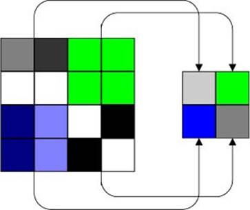
Figure 3.9 Scaling a 4 × 4 image by 0.5
MAX_ARGB = 0xFFFFFFFF
MAX_COMPONENT = 0xFF
The minimum 32-bit ARGB value is 0x0 (i.e., 0x00000000, transparent—strictly speaking, transparent black). These two Image module constants specify the maximum ARGB value (solid white) and the maximum value of any color component (255).
@staticmethod
def argb_for_color(color):
if numpy is not None:
if isinstance(color, numpy.uint32):
color = int(color)
if isinstance(color, str):
color = color_for_name(color)
elif not isinstance(color, int) or not (0 <= color <= MAX_ARGB):
raise Error("invalid color {}".format(color))
α = (color >> 24) & MAX_COMPONENT
r = (color >> 16) & MAX_COMPONENT
g = (color >> 8) & MAX_COMPONENT
b = (color & MAX_COMPONENT)
return α, r, g, b
This static method (and module function) returns the four color components (each in the range 0 to 255) for a given color. The color passed in can be an int, a numpy.uint32, or a str color name. The individual color components (bytes) of the int that represents the color are then extracted (as ints) using bitwise shifts (>>) and bitwise and-ing (&).
@staticmethod
def color_for_name(name):
if name is None:
return ColorForName["transparent"]
if name.startswith("#"):
name = name[1:]
if len(name) == 3: # add solid alpha
name = "F" + name # now has 4 hex digits
if len(name) == 6: # add solid alpha
name = "FF" + name # now has the full 8 hex digits
if len(name) == 4: # originally #FFF or #FFFF
components = []
for h in name:
components.extend([h, h])
name = "".join(components) # now has the full 8 hex digits
return int(name, 16)
return ColorForName[name.lower()]
This static method (and module function) returns a 32-bit ARGB value for a given str color. If the color passed is None, the method returns transparent. If the string begins with #, it is assumed to be an HTML-style color of one of the forms "#HHH", "#HHHH", "#HHHHHH", or"#HHHHHHHH", where H is a hexadecimal digit. If the number of digits supplied is only sufficient for an RGB value, we prefix it with two "F"s to make the color have an opaque alpha channel. Otherwise, we return the color from the ColorForName dictionary; this always succeeds because ColorForName is a default dictionary.
ColorForName = collections.defaultdict(lambda: 0xFF000000, {
"transparent": 0x00000000, "aliceblue": 0xFFF0F8FF,
...
"yellow4": 0xFF8B8B00, "yellowgreen": 0xFF9ACD32})
The ColorForName is a collections.defaultdict that returns a 32-bit unsigned integer that encodes the given named color’s alpha, red, green, and blue color components or, if the name isn’t in the dictionary, silently returns solid black (0xFF000000). Although Image users are free to use this dictionary, the color_ for_name() function is more convenient and versatile. The color names are taken from the rgb.txt file supplied with X11, with the addition of transparent.
The collections.defaultdict() function accepts a factory function as its first argument, followed by any arguments that a plain dict accepts. The factory function is used to produce the value for any item that is brought into existence when a missing key is accessed. Here, we have used a lambda that always returns the same value (solid black). Although it is possible to pass keyword arguments (e.g., transparent=0x00000000), we have more colors than Python’s limit of 255 arguments, so we initialize the default dictionary with a normal dictionary created using the {key: value} syntax, which has no such limit.
argb_for_color = Image.argb_for_color
rgb_for_color = Image.rgb_for_color
color_for_argb = Image.color_for_argb
color_for_rgb = Image.color_for_rgb
color_for_name = Image.color_for_name
After the Image class we have created some convenience functions based on some of the class’s static methods. This means, for example, that after doing import Image, the user can call Image.color_for_name() or, if they have an Image.Image instance,image.color_for_name().
We have now completed our review of the core Image module (in Image/ __init__.py). We have omitted a couple of less interesting constants, a few Image.Image methods (rectangle(), ellipse(), and subsample()), the size property (which just returns a width and height 2-tuple), and various color manipulating static methods. The module is sufficient for creating, loading, drawing on, and saving image files using the XBM and XPM formats, and if the PyPNG module is installed, the PNG format.
Now we will look at two image-format–specific modules that the Image module relies on. We will omit coverage of the Image/Xbm.py module, though, since apart from the low-level details of the XBM format covering it would not teach us any more than we can learn from theImage/Xpm.py module that we will look at next.
3.12.2. An Overview of the Xpm Module
Every image-format–specific module is expected to provide four functions. Two of these are can_load() and can_save(). Both of these functions should return 0 to indicate they can’t, 100 to indicate they can, or some value in between if they can imperfectly. The module is also expected to provide load() and save() functions, and these may assume that they will only ever be called with a filename for which the corresponding can_load() or can_save() function returned a nonzero value.
def can_load(filename):
return 80 if os.path.splitext(filename)[1].lower() == ".xpm" else 0
def can_save(filename):
return can_load(filename)
The Image/Xpm.py module implements most of the XPM specification, leaving out some rarely used features. In view of this, it reports a rating of 80 (i.e., less than perfect), both for loading and saving.* This means that if a new XPM-handling module was added—say asImage/Xpm2.py—providing it reports a rating greater than 80, the new module will be used instead of this one. (We discussed this when we covered the Image._choose_module() method; 129 ![]() .)
.)
*An alternative to checking a file’s type by extension is to read its first few bytes—its “magic” number. For example, XPM files begin with the bytes 0x2F 0x2A 0x20 0x58 0x50 0x4D 0x20 0x2A 0x2F ("/*XPM */") and PNG files with 0x89 0x50 0x4E 0x47 0x0D 0x0A 0x1A 0x0A ("·PNG·#183;··").
(_WANT_XPM, _WANT_NAME, _WANT_VALUES, _WANT_COLOR, _WANT_PIXELS,
_DONE) = ("WANT_XPM", "WANT_NAME", "WANT_VALUES", "WANT_COLOR",
"WANT_PIXELS", "DONE")
_CODES = "".join((chr(x) for x in range(32, 127) if chr(x) not in '\\"'))
The XPM format is a plain text (7-bit ASCII) format that must be parsed to extract its data. The format consists of some metadata (width, height, number of colors, and so on), a color table, and pixel data that identifies each pixel by reference to the color table. The details would take us too far from Python to go into further; however, we use a simple, hand-coded parser, and these constants provide the parser’s states.
def load(image, filename):
colors = cpp = count = None
state = _WANT_XPM
palette = {}
index = 0
with open(filename, "rt", encoding="ascii") as file:
for lino, line in enumerate(file, start=1):
line = line.strip()
...
This is the start of the module’s load() function. The image passed in is of type Image.Image, and inside the function (but not shown), the image’s pixels, width, and height attributes are all set directly. The pixels array is created using the Image.create_array() function so that the Xpm.py module doesn’t have to know or care whether the array is an array.array or a numpy.ndarray, so long as the array is one dimensional and of length width × height. This does mean, though, that we must only access the pixels array using methods that are common to both types.
def save(image, filename):
name = Image.sanitized_name(filename)
palette, cpp = _palette_and_cpp(image.pixels)
with open(filename, "w+t", encoding="ascii") as file:
_write_header(image, file, name, cpp, len(palette))
_write_palette(file, palette)
_write_pixels(image, file, palette)
Both XBM and XPM formats include a name in the actual file that is based on their filename but which must be a valid identifier in the C language. We obtain this name using the Image.sanitized_name() function. Almost all of the saving work is passed on to private helper functions, none of which is of intrinsic interest, and so they aren’t shown.
def sanitized_name(name):
name = re.sub(r"\W+", "", os.path.basename(os.path.splitext(name)[0]))
if not name or name[0].isdigit():
name = "z" + name
return name
The Image.sanitized_name() function takes a filename and produces a name based on it that includes only unaccented Latin letters, digits, and underscores, and that starts with a letter or underscore. In the regex, \W+ matches one or more non-word characters (i.e., characters that are not valid in C identifiers).
Support for any other image format can be added to the Image module by creating a suitable module to go in the Image directory, which has the four required functions: can_load(), can_save(), load(), and save(), where the first two return appropriate integers for the filenames they are given. One very popular image format is PNG format, but it is pretty complicated. Fortunately, we can adapt the existing PyPNG module to take advantage of it with minimal effort, as we will see in the next subsection.
3.12.3. The PNG Wrapper Module
The PyPNG module (github.com/drj11/pypng) provides good support for the PNG image format. However, it doesn’t have the interface that the Image module requires for an image-specific format module. So, in this subsection we will create the Image/Png.py module, which will use the Adapter Pattern (§2.1, 29 ![]() ) to add support for PNG images to the Image module. And unlike the previous subsection, where we only showed a small sample of the code, here we will see all of the Image/Png.py module’s code.
) to add support for PNG images to the Image module. And unlike the previous subsection, where we only showed a small sample of the code, here we will see all of the Image/Png.py module’s code.
try:
import png
except ImportError:
png = None
We begin by attempting to import PyPNG’s png module. If this fails we create a png variable of value None that we can check later.
def can_load(filename):
return (80 if png is not None and
os.path.splitext(filename)[1].lower() == ".png" else 0)
def can_save(filename):
return can_load(filename)
If the png module was successfully imported, we return a rating of 80 (slightly imperfect) as our indication of this module’s PNG support. We use 80 rather than 100 to allow for another module to supercede this one. Just as for the XPM format, we return the same rating for both loading and saving; however, it is perfectly acceptable to return different ratings.