Dependence and Independence

Roughly speaking, we say that two events E and F are dependent if knowing something about whether E happens gives us information about whether F happens (and vice versa). Otherwise they are independent.

For instance, if we flip a fair coin twice, knowing whether the first flip is Heads gives us no information about whether the second flip is Heads. These events are independent. On the other hand, knowing whether the first flip is Heads certainly gives us information about whether both flips are Tails. (If the first flip is Heads, then definitely it’s not the case that both flips are Tails.) These two events are dependent.

Mathematically, we say that two events E and F are independent if the probability that they both happen is the product of the probabilities that each one happens:

In the example above, the probability of “first flip Heads” is 1/2, and the probability of “both flips Tails” is 1/4, but the probability of “first flip Heads and both flips Tails” is 0.

Conditional Probability

When two events E and F are independent, then by definition we have:

If they are not necessarily independent (and if the probability of F is not zero), then we define the probability of E “conditional on F” as:

You should think of this as the probability that E happens, given that we know that F happens.

We often rewrite this as:

When E and F are independent, you can check that this gives:

which is the mathematical way of expressing that knowing F occurred gives us no additional information about whether E occurred.

One common tricky example involves a family with two (unknown) children.

If we assume that:

1. Each child is equally likely to be a boy or a girl

2. The gender of the second child is independent of the gender of the first child

then the event “no girls” has probability 1/4, the event “one girl, one boy” has probability 1/2, and the event “two girls” has probability 1/4.

Now we can ask what is the probability of the event “both children are girls” (B) conditional on the event “the older child is a girl” (G)? Using the definition of conditional probability:

since the event B and G (“both children are girls and the older child is a girl”) is just the event B. (Once you know that both children are girls, it’s necessarily true that the older child is a girl.)

Most likely this result accords with your intuition.

We could also ask about the probability of the event “both children are girls” conditional on the event “at least one of the children is a girl” (L). Surprisingly, the answer is different from before!

As before, the event B and L (“both children are girls and at least one of the children is a girl”) is just the event B. This means we have:

How can this be the case? Well, if all you know is that at least one of the children is a girl, then it is twice as likely that the family has one boy and one girl than that it has both girls.

We can check this by “generating” a lot of families:

def random_kid():

    return random.choice(["boy", "girl"])

both_girls = 0

older_girl = 0

either_girl = 0

random.seed(0)

for _ in range(10000):

    younger = random_kid()

    older = random_kid()

    if older == "girl":

        older_girl += 1

    if older == "girl" and younger == "girl":

        both_girls += 1

    if older == "girl" or younger == "girl":

        either_girl += 1

print "P(both | older):", both_girls / older_girl      # 0.514 ~ 1/2

print "P(both | either): ", both_girls / either_girl   # 0.342 ~ 1/3

Bayes’s Theorem

One of the data scientist’s best friends is Bayes’s Theorem, which is a way of “reversing” conditional probabilities. Let’s say we need to know the probability of some event E conditional on some other event F occurring. But we only have information about the probability of F conditional on E occurring. Using the definition of conditional probability twice tells us that:

The event F can be split into the two mutually exclusive events “F and E” and “F and not E.” If we write for “not E” (i.e., “E doesn’t happen”), then:

so that:

which is how Bayes’s Theorem is often stated.

This theorem often gets used to demonstrate why data scientists are smarter than doctors. Imagine a certain disease that affects 1 in every 10,000 people. And imagine that there is a test for this disease that gives the correct result (“diseased” if you have the disease, “nondiseased” if you don’t) 99% of the time.

What does a positive test mean? Let’s use T for the event “your test is positive” and D for the event “you have the disease.” Then Bayes’s Theorem says that the probability that you have the disease, conditional on testing positive, is:

Here we know that , the probability that someone with the disease tests positive, is 0.99. , the probability that any given person has the disease, is 1/10,000 = 0.0001. , the probability that someone without the disease tests positive, is 0.01. And , the probability that any given person doesn’t have the disease, is 0.9999. If you substitute these numbers into Bayes’s Theorem you find

That is, less than 1% of the people who test positive actually have the disease.

NOTE

This assumes that people take the test more or less at random. If only people with certain symptoms take the test we would instead have to condition on the event “positive test and symptoms” and the number would likely be a lot higher.

While this is a simple calculation for a data scientist, most doctors will guess that is approximately 2.

A more intuitive way to see this is to imagine a population of 1 million people. You’d expect 100 of them to have the disease, and 99 of those 100 to test positive. On the other hand, you’d expect 999,900 of them not to have the disease, and 9,999 of those to test positive. Which means that you’d expect only 99 out of (99 + 9999) positive testers to actually have the disease.

Random Variables

A random variable is a variable whose possible values have an associated probability distribution. A very simple random variable equals 1 if a coin flip turns up heads and 0 if the flip turns up tails. A more complicated one might measure the number of heads observed when flipping a coin 10 times or a value picked from range(10) where each number is equally likely.

The associated distribution gives the probabilities that the variable realizes each of its possible values. The coin flip variable equals 0 with probability 0.5 and 1 with probability 0.5. The range(10) variable has a distribution that assigns probability 0.1 to each of the numbers from 0 to 9.

We will sometimes talk about the expected value of a random variable, which is the average of its values weighted by their probabilities. The coin flip variable has an expected value of 1/2 (= 0 * 1/2 + 1 * 1/2), and the range(10) variable has an expected value of 4.5.

Random variables can be conditioned on events just as other events can. Going back to the two-child example from “Conditional Probability”, if X is the random variable representing the number of girls, X equals 0 with probability 1/4, 1 with probability 1/2, and 2 with probability 1/4.

We can define a new random variable Y that gives the number of girls conditional on at least one of the children being a girl. Then Y equals 1 with probability 2/3 and 2 with probability 1/3. And a variable Z that’s the number of girls conditional on the older child being a girl equals 1 with probability 1/2 and 2 with probability 1/2.

For the most part, we will be using random variables implicitly in what we do without calling special attention to them. But if you look deeply you’ll see them.

Continuous Distributions

A coin flip corresponds to a discrete distribution — one that associates positive probability with discrete outcomes. Often we’ll want to model distributions across a continuum of outcomes. (For our purposes, these outcomes will always be real numbers, although that’s not always the case in real life.) For example, the uniform distribution puts equal weight on all the numbers between 0 and 1.

Because there are infinitely many numbers between 0 and 1, this means that the weight it assigns to individual points must necessarily be zero. For this reason, we represent a continuous distribution with a probability density function (pdf) such that the probability of seeing a value in a certain interval equals the integral of the density function over the interval.

NOTE

If your integral calculus is rusty, a simpler way of understanding this is that if a distribution has density function , then the probability of seeing a value between and is approximately if is small.

The density function for the uniform distribution is just:

def uniform_pdf(x):

    return 1 if x >= 0 and x < 1 else 0

The probability that a random variable following that distribution is between 0.2 and 0.3 is 1/10, as you’d expect. Python’s random.random() is a [pseudo]random variable with a uniform density.

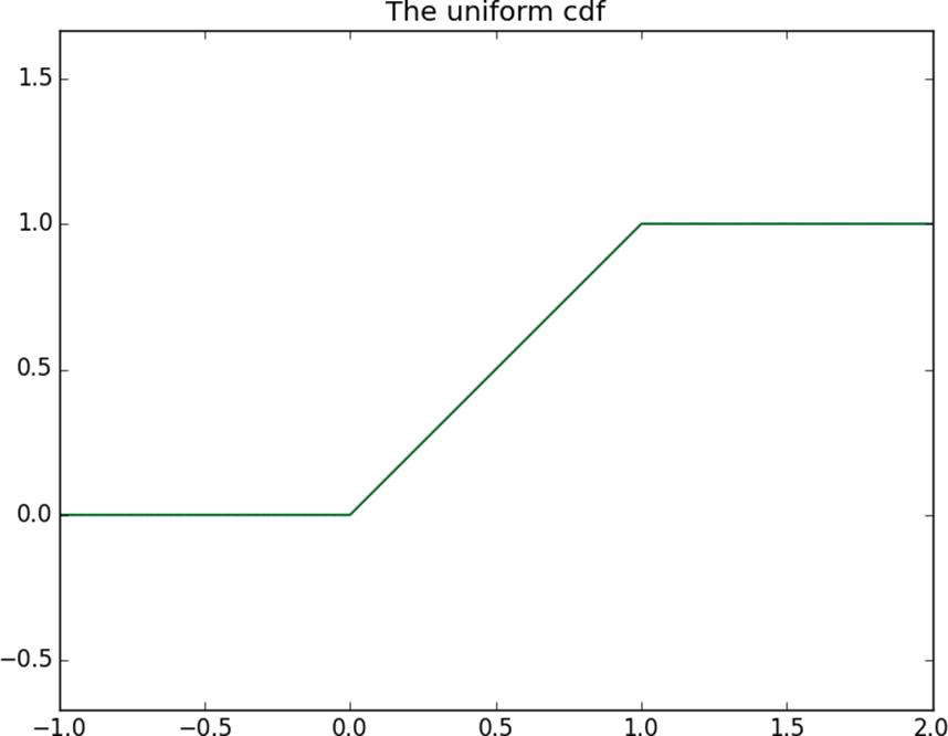
We will often be more interested in the cumulative distribution function (cdf), which gives the probability that a random variable is less than or equal to a certain value. It’s not hard to create the cumulative distribution function for the uniform distribution (Figure 6-1):

def uniform_cdf(x):

    "returns the probability that a uniform random variable is <= x"

    if x < 0:   return 0    # uniform random is never less than 0

    elif x < 1: return x    # e.g. P(X <= 0.4) = 0.4

    else:       return 1    # uniform random is always less than 1

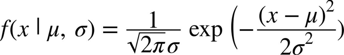
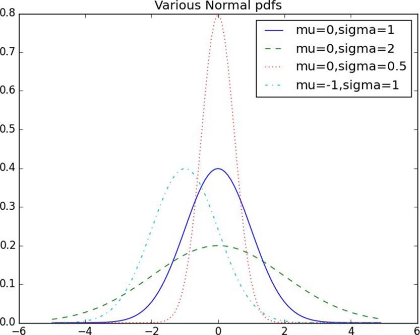
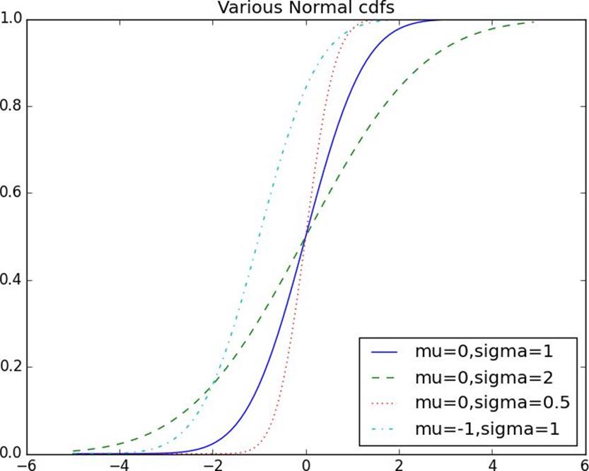
The normal distribution is the king of distributions. It is the classic bell curve-shaped distribution and is completely determined by two parameters: its mean (mu) and its standard deviation (sigma). The mean indicates where the bell is centered, and the standard deviation how “wide” it is.

It has the distribution function:

which we can implement as:

def normal_pdf(x, mu=0, sigma=1):

    sqrt_two_pi = math.sqrt(2 * math.pi)

    return (math.exp(-(x-mu) ** 2 / 2 / sigma ** 2) / (sqrt_two_pi * sigma))

In Figure 6-2, we plot some of these pdfs to see what they look like:

xs = [x / 10.0 for x in range(-50, 50)]

plt.plot(xs,[normal_pdf(x,sigma=1) for x in xs],'-',label='mu=0,sigma=1')

plt.plot(xs,[normal_pdf(x,sigma=2) for x in xs],'--',label='mu=0,sigma=2')

plt.plot(xs,[normal_pdf(x,sigma=0.5) for x in xs],':',label='mu=0,sigma=0.5')

plt.plot(xs,[normal_pdf(x,mu=-1)   for x in xs],'-.',label='mu=-1,sigma=1')

plt.legend()

plt.title("Various Normal pdfs")

plt.show()

When and , it’s called the standard normal distribution. If Z is a standard normal random variable, then it turns out that:

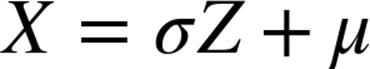
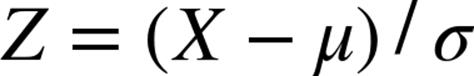
is also normal but with mean and standard deviation . Conversely, if X is a normal random variable with mean and standard deviation ,

is a standard normal variable.

The cumulative distribution function for the normal distribution cannot be written in an “elementary” manner, but we can write it using Python’s math.erf:

def normal_cdf(x, mu=0,sigma=1):

    return (1 + math.erf((x - mu) / math.sqrt(2) / sigma)) / 2

Again, in Figure 6-3, we plot a few:

xs = [x / 10.0 for x in range(-50, 50)]

plt.plot(xs,[normal_cdf(x,sigma=1) for x in xs],'-',label='mu=0,sigma=1')

plt.plot(xs,[normal_cdf(x,sigma=2) for x in xs],'--',label='mu=0,sigma=2')

plt.plot(xs,[normal_cdf(x,sigma=0.5) for x in xs],':',label='mu=0,sigma=0.5')

plt.plot(xs,[normal_cdf(x,mu=-1) for x in xs],'-.',label='mu=-1,sigma=1')

plt.legend(loc=4) # bottom right

plt.title("Various Normal cdfs")

plt.show()

Sometimes we’ll need to invert normal_cdf to find the value corresponding to a specified probability. There’s no simple way to compute its inverse, but normal_cdf is continuous and strictly increasing, so we can use a binary search:

def inverse_normal_cdf(p, mu=0, sigma=1, tolerance=0.00001):

    """find approximate inverse using binary search"""

    # if not standard, compute standard and rescale

    if mu != 0 or sigma != 1:

        return mu + sigma * inverse_normal_cdf(p, tolerance=tolerance)

    low_z, low_p = -10.0, 0            # normal_cdf(-10) is (very close to) 0

    hi_z,  hi_p  =  10.0, 1            # normal_cdf(10)  is (very close to) 1

    while hi_z - low_z > tolerance:

        mid_z = (low_z + hi_z) / 2     # consider the midpoint

        mid_p = normal_cdf(mid_z)      # and the cdf's value there

        if mid_p < p:

            # midpoint is still too low, search above it

            low_z, low_p = mid_z, mid_p

        elif mid_p > p:

            # midpoint is still too high, search below it

            hi_z, hi_p = mid_z, mid_p

        else:

            break

    return mid_z

The function repeatedly bisects intervals until it narrows in on a Z that’s close enough to the desired probability.

The Central Limit Theorem

One reason the normal distribution is so useful is the central limit theorem, which says (in essence) that a random variable defined as the average of a large number of independent and identically distributed random variables is itself approximately normally distributed.

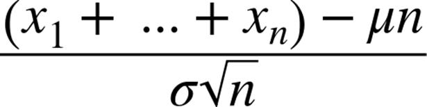
In particular, if are random variables with mean and standard deviation , and if n is large, then:

is approximately normally distributed with mean and standard deviation . Equivalently (but often more usefully),

is approximately normally distributed with mean 0 and standard deviation 1.

An easy way to illustrate this is by looking at binomial random variables, which have two parameters n and p. A Binomial(n,p) random variable is simply the sum of n independent Bernoulli(p) random variables, each of which equals 1 with probability p and 0 with probability :

def bernoulli_trial(p):

    return 1 if random.random() < p else 0

def binomial(n, p):

    return sum(bernoulli_trial(p) for _ in range(n))

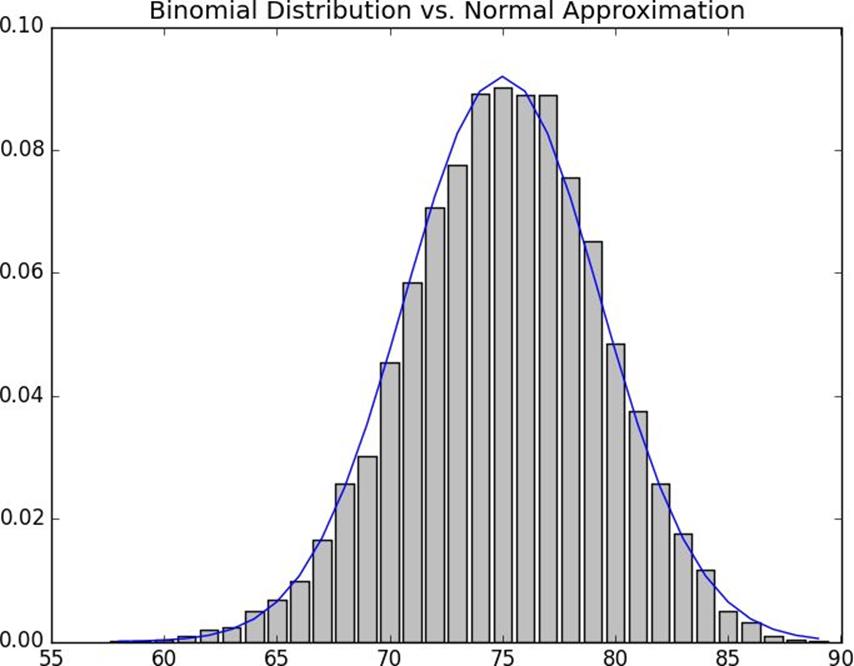
The mean of a Bernoulli(p) variable is p, and its standard deviation is . The central limit theorem says that as n gets large, a Binomial(n,p) variable is approximately a normal random variable with mean and standard deviation . If we plot both, you can easily see the resemblance:

def make_hist(p, n, num_points):

    data = [binomial(n, p) for _ in range(num_points)]

    # use a bar chart to show the actual binomial samples

    histogram = Counter(data)

    plt.bar([x - 0.4 for x in histogram.keys()],

            [v / num_points for v in histogram.values()],

            0.8,

            color='0.75')

    mu = p * n

    sigma = math.sqrt(n * p * (1 - p))

    # use a line chart to show the normal approximation

    xs = range(min(data), max(data) + 1)

    ys = [normal_cdf(i + 0.5, mu, sigma) - normal_cdf(i - 0.5, mu, sigma)

          for i in xs]

    plt.plot(xs,ys)

    plt.title("Binomial Distribution vs. Normal Approximation")

    plt.show()

For example, when you call make_hist(0.75, 100, 10000), you get the graph in Figure 6-4.

The moral of this approximation is that if you want to know the probability that (say) a fair coin turns up more than 60 heads in 100 flips, you can estimate it as the probability that a Normal(50,5) is greater than 60, which is easier than computing the Binomial(100,0.5) cdf. (Although in most applications you’d probably be using statistical software that would gladly compute whatever probabilities you want.)

For Further Exploration

§ scipy.stats contains pdf and cdf functions for most of the popular probability distributions.

§ Remember how, at the end of Chapter 5, I said that it would be a good idea to study a statistics textbook? It would also be a good idea to study a probability textbook. The best one I know that’s available online is Introduction to Probability.