Foundations of Algorithms (2015)

Chapter 1 Algorithms: Efficiency, Analysis, and Order

This text is about techniques for solving problems using a computer. By “technique” we do not mean a programming style or a programming language but rather the approach or methodology used to solve a problem. For example, suppose Barney Beagle wants to find the name “Collie, Colleen” in the phone book. One approach is to check each name in sequence, starting with the first name, until “Collie, Colleen” is located. No one, however, searches for a name this way. Instead, Barney takes advantage of the fact that the names in the phone book are sorted and opens the book to where he thinks the C’s are located. If he goes too far into the book, he thumbs back a little. He continues thumbing back and forth until he locates the page containing “Collie, Colleen.” You may recognize this second approach as a modified binary search and the first approach as a sequential search. We discuss these searches further in Section 1.2. The point here is that we have two distinct approaches to solving the problem, and the approaches have nothing to do with a programming language or style. A computer program is simply one way to implement these approaches.

Chapters 2 through 6 discuss various problem-solving techniques and apply those techniques to a variety of problems. Applying a technique to a problem results in a step-by-step procedure for solving the problem. This step-by-step procedure is called an algorithm for the problem. The purpose of studying these techniques and their applications is so that, when confronted with a new problem, you have a repertoire of techniques to consider as possible ways to solve the problem. We will often see that a given problem can be solved using several techniques but that one technique results in a much faster algorithm than the others. Certainly, a modified binary search is faster than a sequential search when it comes to finding a name in a phone book. Therefore, we will be concerned not only with determining whether a problem can be solved using a given technique but also with analyzing how efficient the resulting algorithm is in terms of time and storage. When the algorithm is implemented on a computer, time means CPU cycles and storage means memory. You may wonder why efficiency should be a concern, because computers keep getting faster and memory keeps getting cheaper. In this chapter, we discuss some fundamental concepts necessary to the material in the rest of the text. Along the way, we show why efficiency always remains a consideration, regardless of how fast computers get and how cheap memory becomes.

1.1 Algorithms

So far we have mentioned the words “problem,” “solution,” and “algorithm.” Most of us have a fairly good idea of what these words mean. However, to lay a sound foundation, let’s define these terms concretely.

A computer program is composed of individual modules, understandable by a computer, that solve specific tasks (such as sorting). Our concern in this text is not the design of entire programs, but rather the design of the individual modules that accomplish the specific tasks. These specific tasks are called problems. Explicitly, we say that a problem is a question to which we seek an answer. Examples of problems follow.

Example 1.1

The following is an example of a problem:

Sort a list S of n numbers in nondecreasing order. The answer is the numbers in sorted sequence.

By a list we mean a collection of items arranged in a particular sequence. For example,

is a list of six numbers in which the first number is 10, the second is 7, and so on. In Example 1.1 we say the list is to be sorted in “nondecreasing order” instead of increasing order to allow for the possibility that the same number may appear more than once in the list.

Example 1.2

The following is an example of a problem:

Determine whether the number x is in the list S of n numbers. The answer is yes if x is in S and no if it is not.

A problem may contain variables that are not assigned specific values in the statement of the problem. These variables are called parameters to the problem. In Example 1.1 there are two parameters: S (the list) and n (the number of items in S). In Example 1.2 there are three parameters: S, n, and the number x. It is not necessary in these two examples to make n one of the parameters because its value is uniquely determined by S. However, making n a parameter facilitates our descriptions of problems.

Because a problem contains parameters, it represents a class of problems, one for each assignment of values to the parameters. Each specific assignment of values to the parameters is called an instance of the problem. A solution to an instance of a problem is the answer to the question asked by the problem in that instance.

Example 1.3

An instance of the problem in Example 1.1 is

The solution to this instance is [5, 7, 8, 10, 11, 13].

Example 1.4

An instance of the problem in Example 1.2 is

The solution to this instance is, “yes, x is in S.”

We can find the solution to the instance in Example 1.3 by inspecting S and allowing the mind to produce the sorted sequence by cognitive steps that cannot be specifically described. This can be done because S is so small that at a conscious level, the mind seems to scan S rapidly and produce the solution almost immediately (and therefore one cannot describe the steps the mind follows to obtain the solution). However, if the instance had a value of 1,000 for n, a person would not be able to use this method, and it certainly would not be possible to convert such a method of sorting numbers to a computer program. To produce a computer program that can solve all instances of a problem, we must specify a general step-by-step procedure for producing the solution to each instance. This step-by-step procedure is called an algorithm. We say that the algorithm solves the problem.

Example 1.5

An algorithm for the problem in Example 1.2 is as follows. Starting with the first item in S, compare x with each item in S in sequence until x is found or until S is exhausted. If x is found, answer yes; if x is not found, answer no.

We can communicate any algorithm in the English language as we did in Example 1.5. However, there are two drawbacks to writing algorithms in this manner. First, it is difficult to write a complex algorithm this way, and even if we did, a person would have a difficult time understanding the algorithm. Second, it is not clear how to create a computer language description of an algorithm from an English language description of it.

Because C++ is a language with which students are currently familiar, we use a C++-like pseudocode to write algorithms. Anyone with programming experience in an Algol-like imperative language such as C, Pascal, or Java should have no difficulty with the pseudocode.

We illustrate the pseudocode with an algorithm that solves a generalization of the problem in Example 1.2. For simplicity, Examples 1.1 and 1.2 were stated for numbers. However, in general we want to search and sort items that come from any ordered set. Often each item uniquely identifies a record, and therefore we commonly call the items keys. For example, a record may consist of personal information about an individual and have the person’s social security number as its key. We write searching and sorting algorithms using the defined data type keytype for the items. It means the items are from any ordered set.

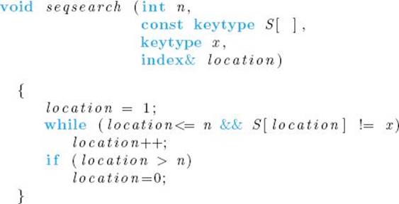
The following algorithm represents the list S by an array and, instead of merely returning yes or no, returns x’s location in the array if x is in S and returns 0 otherwise. This particular searching algorithm does not require that the items come from an ordered set, but we still use our standard data type keytype.

Algorithm 1.1

Sequential Search

Problem: Is the key x in the array S of n keys?

Inputs (parameters): positive integer n, array of keys S indexed from 1 to n, and a key x.

Outputs: location, the location of x in S (0 if x is not in S).

The pseudocode is similar, but not identical, to C++. A notable exception is our use of arrays. C++ allows arrays to be indexed only by integers starting at 0. Often we can explain algorithms more clearly using arrays indexed by other integer ranges, and sometimes we can explain them best using indices that are not integers at all. So in pseudocode we allow arbitrary sets to index our arrays. We always specify the ranges of indices in the Inputs and Outputs specifications for the algorithm. For example, in Algorithm 1.1 we specified that S is indexed from 1 to n. Since we are used to counting the items in a list starting with 1, this is a good index range to use for a list. Of course, this particular algorithm can be implemented directly in C++ by declaring

and simply not using the S[0] slot. Hereafter, we will not discuss the implementation of algorithms in any particular programming language. Our purpose is only to present algorithms clearly so they can be readily understood and analyzed.

There are two other significant deviations from C++ regarding arrays in pseudocode. First, we allow variable-length two-dimensional arrays as parameters to routines. See, for example, Algorithm 1.4 on page 8. Second, we declare local variable-length arrays. For example, if n is a parameter to procedure example, and we need a local array indexed from 2 to n, we declare

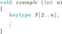
The notation S[2..n] means an array S indexed from 2 to n is strictly pseudocode; that is, it is not part of the C++ language.

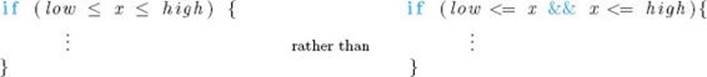
Whenever we can demonstrate steps more succinctly and clearly using mathematical expressions or English-like descriptions than we could using actual C++ instructions, we do so. For example, suppose some instructions are to be executed only if a variable x is between the values low and high. We write

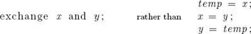
Suppose we wanted the variable x to take the value of variable y and y to take the value of x. We write

Besides the data type keytype, we often use the following, which also are not predefined C++ data types:

We use the data type number when it is not important to the algorithm whether the numbers can take any real values or are restricted to the integers.

Sometimes we use the following nonstandard control structure:

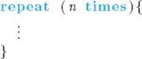
This means repeat the code n times. In C++ it would be necessary to introduce an extraneous control variable and write a for loop. We only use a for loop when we actually need to refer to the control variable within the loop.

When the name of an algorithm seems appropriate for a value it returns, we write the algorithm as a function. Otherwise, we write the algorithm as a procedure (void function in C++) and use reference parameters (that is, parameters that are passed by address) to return values. If the parameter is not an array, it is declared with an ampersand (&) at the end of the data type name. For our purposes, this means that the parameter contains a value returned by the algorithm. Because arrays are automatically passed by reference in C++ and the ampersand is not used in C++ when passing arrays, we do not use the ampersand to indicate that an array contains values returned by thc algorithm. Instead, since the reserved word const is used in C++ to prevent modification of a passed array, we use const to indicate that the array does not contain values returned by the algorithm.

In general, we avoid features peculiar to C++ so that the pseudocode is accessible to someone who knows only another high-level language. However, we do write instructions like i++, which means increment i by 1.

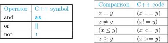
If you do not know C++, you may find the notation used for logical operators and certain relational operators unfamiliar. This notation is as follows:

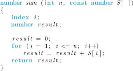
More example algorithms follow. The first shows the use of a function. While procedures have the keyword void before the routine’s name, functions have the data type returned by the function before the routine’s name. The value is returned in the function via the return statement.

Algorithm 1.2

Add Array Members

Problem: Add all the numbers in the array S of n numbers.

Inputs: positive integer n, array of numbers S indexed from 1 to n.

Outputs: sum, the sum of the numbers in S.

We discuss many sorting algorithms in this text. A simple one follows.

Algorithm 1.3

Exchange Sort

Problem: Sort n keys in nondecreasing order.

Inputs: positive integer n, array of keys S indexed from 1 to n.

Outputs: the array S containing the keys in nondecreasing order.

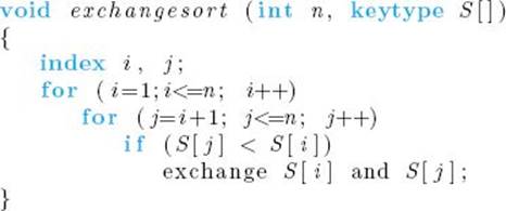
The instruction

exchange S [ i ] and S [ j ] ;

means that S[i] is to take the value of S[j], and S[j] is to take the value of S[i]. This command looks nothing like a C++ instruction; whenever we can state something more simply by not using the details of C++ instructions we do so. Exchange Sort works by comparing the number in the ith slot with the numbers in the (i + 1)st through nth slots. Whenever a number in a given slot is found to be smaller than the one in the ith slot, the two numbers are exchanged. In this way, the smallest number ends up in the first slot after the first pass through for-i loop, the second-smallest number ends up in the second slot after the second pass, and so on.

The next algorithm does matrix multiplication. Recall that if we have two 2 × 2 matrices,

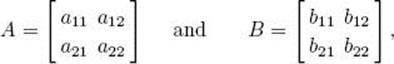
their product C = A × B is given by

For example,

In general, if we have two n × n matrices A and B, their product C is given by

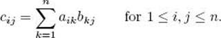
Directly from this definition, we obtain the following algorithm for matrix multiplication.

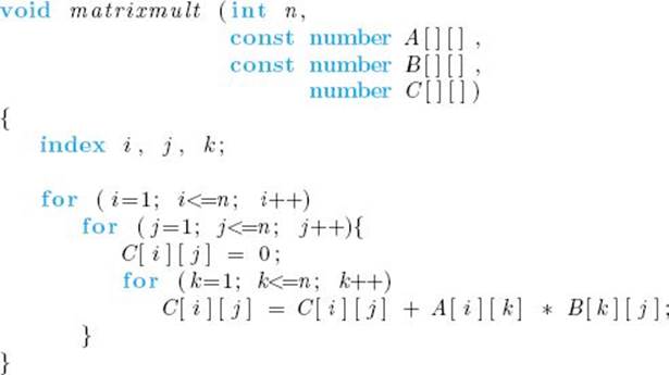
Algorithm 1.4

Matrix Multiplication

Problem: Determine the product of two n × n matrices.

Inputs: a positive integer n, two-dimensional arrays of numbers A and B, each of which has both its rows and columns indexed from 1 to n.

Outputs: a two-dimensional array of numbers C, which has both its rows and columns indexed from 1 to n, containing the product of A and B.

1.2 The Importance of Developing Efficient Algorithms

Previously we mentioned that, regardless of how fast computers become or how cheap memory gets, efficiency will always remain an important consideration. Next we show why this is so by comparing two algorithms for the same problem.

• 1.2.1 Sequential Search Versus Binary Search

Earlier we mentioned that the approach used to find a name in the phone book is a modified binary search, and it is usually much faster than a sequential search. Next we compare algorithms for the two approaches to show how much faster the binary search is.

We have already written an algorithm that does a sequential search— namely, Algorithm 1.1. An algorithm for doing a binary search of an array that is sorted in nondecreasing order is similar to thumbing back and forth in a phone book. That is, given that we are searching for x, the algorithm first compares x with the middle item of the array. If they are equal, the algorithm is done. If x is smaller than the middle item, then x must be in the first half of the array (if it is present at all), and the algorithm repeats the searching procedure on the first half of the array. (That is, x is compared with the middle item of the first half of the array. If they are equal, the algorithm is done, etc.) If x is larger than the middle item of the array, the search is repeated on the second half of the array. This procedure is repeated until x is found or it is determined that x is not in the array. An algorithm for this method follows.

Algorithm 1.5

Binary Search

Problem: Determine whether x is in the sorted array S of n keys.

Inputs: positive integer n, sorted (nondecreasing order) array of keys S indexed from 1 to n, a key x.

Outputs: location, the location of x in S (0 if x is not in S).

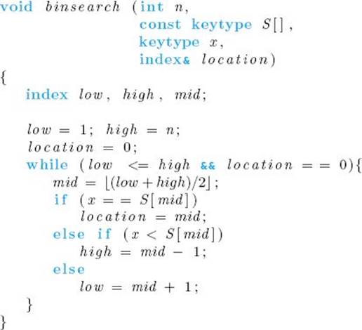
Let’s compare the work done by Sequential Search and Binary Search. For focus we will determine the number of comparisons done by each algorithm. If the array S contains 32 items and x is not in the array, Algorithm 1.1 (Sequential Search) compares x with all 32 items before determining that x is not in the array. In general, Sequential Search does n comparisons to determine that x is not in an array of size n. It should be clear that this is the largest number of comparisons Sequential Search ever makes when searching an array of size n. That is, if x is in the array, the number of comparisons is no greater than n.

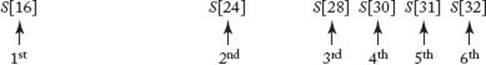
Next consider Algorithm 1.5 (Binary Search). There are two comparisons of x with S[mid] in each pass through the while loop (except when x is found). In an efficient assembler language implementation of the algorithm, x would be compared with S[mid] only once in each pass, the result of that comparison would set the condition code, and the appropriate branch would take place based on the value of the condition code. This means that there would be only one comparison of x with S[mid] in each pass through the while loop. We will assume the algorithm is implemented in this manner. With this assumption, Figure 1.1 shows that the algorithm does six comparisons when x is larger than all the items in an array of size 32. Notice that 6 = lg 32 + 1. By “lg” we mean log₂. The log₂ is encountered so often in analysis of algorithms that we reserve the special symbol lg for it. You should convince yourself that this is the largest number of comparisons Binary Search ever does. That is, if x is in the array, or if x is smaller than all the array items, or if x is between two array items, the number of comparisons is no greater than when x is larger than all the array items.

Suppose we double the size of the array so that it contains 64 items. Binary Search does only one comparison more because the first comparison cuts the array in half, resulting in a subarray of size 32 that is searched. Therefore, when x is larger than all the items in an array of size 64, Binary Search does seven comparisons. Notice that 7 = lg 64 + 1. In general, each time we double the size of the array we add only one comparison. Therefore, if n is a power of 2 and x is larger than all the items in an array of size n, the number of comparisons done by Binary Search is lg n + 1.

Table 1.1 compares the number of comparisons done by Sequential Search and Binary Search for various values of n, when x is larger than all the items in the array. When the array contains around 4 billion items (about the number of people in the world), Binary Search does only 33 comparisons, whereas Sequential Search compares x with all 4 billion items. Even if the computer was capable of completing one pass through the while loop in a nanosecond (one billionth of a second), Sequential Search would take 4 seconds to determine that x is not in the array, whereas Binary Search would make that determination almost instantaneously. This difference would be significant in an online application or if we needed to search for many items.

Figure 1.1 The array items that Binary Search compares with x when x is larger than all the items in an array of size 32. The items are numbered according to the order in which they are compared.

• Table 1.1 The number of comparisons done by Sequential Search and Binary Search when x is larger than all the array items

For convenience, we considered only arrays whose sizes were powers of 2 in the previous discussion of Binary Search. In Chapter 2 we will return to Binary Search as an example of the divide-and-conquer approach, which is the focus of that chapter. At that time we will consider arrays whose sizes can be any positive integer.

As impressive as the searching example is, it is not absolutely compelling because Sequential Search still gets the job done in an amount of time tolerable to a human life span. Next we will look at an inferior algorithm that does not get the job done in a tolerable amount of time.

• 1.2.2 The Fibonacci Sequence

The algorithms discussed here compute the nth term of the Fibonacci sequence, which is defined recursively as follows:

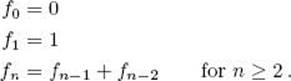
Computing the first few terms, we have

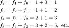
There are various applications of the Fibonacci sequence in computer science and mathematics. Because the Fibonacci sequence is defined recursively, we obtain the following recursive algorithm from the definition.

Algorithm 1.6

nth Fibonacci Term (Recursive)

Problem: Determine the nth term in the Fibonacci sequence.

Inputs: a nonnegative integer n.

Outputs: fib, the nth term of the Fibonacci sequence.

By “nonnegative integer” we mean an integer that is greater than or equal to 0, whereas by “positive integer” we mean an integer that is strictly greater than 0. We specify the input to the algorithm in this manner to make it clear what values the input can take. However, for the sake of avoiding clutter, we declare n simply as an integer in the expression of the algorithm. We will follow this convention throughout the text.

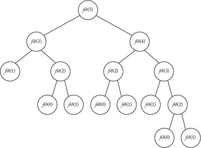
Although the algorithm was easy to create and is understandable, it is extremely inefficient. Figure 1.2 shows the recursion tree corresponding to the algorithm when computing fib(5). The children of a node in the tree contain the recursive calls made by the call at the node. For example, to obtainfib(5) at the top level we need fib(4) and fib(3); then to obtain fib(3) we need fib(2) and fib(l), and so on. As the tree shows, the function is inefficient because values are computed over and over again. For example, fib(2) is computed three times.

How inefficient is this algorithm? The tree in Figure 1.2 shows that the algorithm computes the following numbers of terms to determine fib(n) for 0 ≤ n ≤ 6:

The first six values can be obtained by counting the nodes in the subtree rooted at fib(n) for 1 ≤ n ≤ 5, whereas the number of terms for fib(6) is the sum of the nodes in the trees rooted at fib(5) and fib(4) plus the one node at the root. These numbers do not suggest a simple expression like the one obtained for Binary Search. Notice, however, that in the case of the first seven values, the number of terms in the tree more than doubles every time n increases by 2. For example, there are nine terms in the tree when n = 4 and 25 terms when n = 6. Let’s call T(n) the number of terms in the recursion tree for n. If the number of terms more than doubled every time n increased by 2, we would have the following for n even:

Figure 1.2 The recursion tree corresponding to Algorithm 1.6 when computing the fifth Fibonacci term.

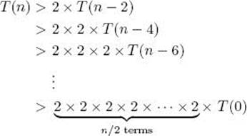
Because T(0) = 1, this would mean T(n) > 2^n/2. We use induction to show that this is true for n ≥ 2 even if n is not even. The inequality does not hold for n = 1 because T(1) = 1, which is less than 2^1/2. Induction is reviewed in Section A.3 in Appendix A.

Theorem 1.1

If T(n) is the number of terms in the recursion tree corresponding to Algorithm 1.6, then, for n ≥ 2,

Proof: The proof is by induction on n.

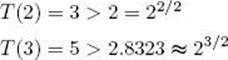
Induction base: We need two base cases because the induction step assumes the results of two previous cases. For n = 2 and n = 3, the recursion in Figure 1.2 shows that

Induction hypothesis: One way to make the induction hypothesis is to assume that the statement is true for all m < n. Then, in the induction step, show that this implies that the statement must be true for n. This technique is used in this proof. Suppose for all m such that 2 ≤ m < n

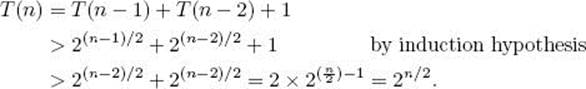
Induction step: We must show that T(n) > 2^n/2. The value of T(n) is the sum of T(n − 1) and T(n − 2) plus the one node at the root. Therefore,

We established that the number of terms computed by Algorithm 1.6 to determine the nth Fibonacci term is greater than 2^n/2. We will return to this result to show how inefficient the algorithm is. But first let’s develop an efficient algorithm for computing the nth Fibonacci term. Recall that the problem with the recursive algorithm is that the same value is computed over and over. As Figure 1.2 shows, fib(2) is computed three times in determining fib(5). If when computing a value, we save it in an array, then whenever we need it later we do not need to recompute it. The following iterative algorithm uses this strategy.

Algorithm 1.7

nth Fibonacci Term (Iterative)

Problem: Determine the nth term in the Fibonacci sequence.

Inputs: a nonnegative integer n.

Outputs: fib2, the nth term in the Fibonacci sequence.

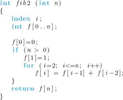
Algorithm 1.7 can be written without using the array f because only the two most recent terms are needed in each iteration of the loop. However, it is more clearly illustrated using the array.

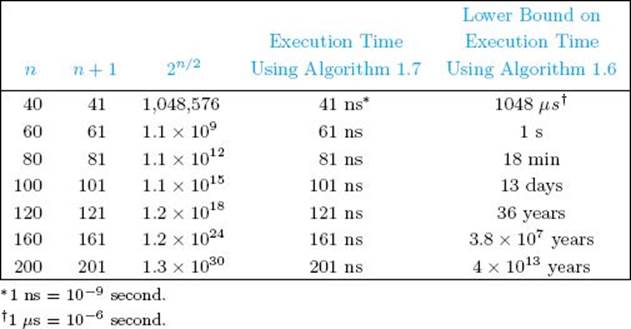
To determine fib2(n), the previous algorithm computes every one of the first n + 1 terms just once. So it computes n + 1 terms to determine the nth Fibonacci term. Recall that Algorithm 1.6 computes more than 2^n/2 terms to determine the nth Fibonacci term. Table 1.2 compares these expressions for various values of n. The execution times are based on the simplifying assumption that one term can be computed in 10⁻⁹ second. The table shows the time it would take Algorithm 1.7 to compute the nth term on a hypothetical computer that could compute each term in a nanosecond, and it shows a lower bound on the time it would take to execute Algorithm 1.7. By the time n is 80, Algorithm 1.6 takes at least 18 minutes. When n is 120, it takes more than 36 years, an amount of time intolerable compared with a human life span. Even if we could build a computer one billion times as fast, Algorithm 1.6 would take over 40,000 years to compute the 200th term. This result can be obtained by dividing the time for the 200th term by one billion. We see that regardless of how fast computers become, Algorithm 1.6 will still take an intolerable amount of time unless n is small. On the other hand, Algorithm 1.7 computes the nth Fibonacci term almost instantaneously. This comparison shows why the efficiency of an algorithm remains an important consideration regardless of how fast computers become.

• Table 1.2 A comparison of Algorithms 1.6 and 1.7

Algorithm 1.6 is a divide-and-conquer algorithm. Recall that the divide-and-conquer approach produced a very efficient algorithm (Algorithm 1.5: Binary Search) for the problem of searching a sorted array. As shown in Chapter 2, the divide-and-conquer approach leads to very efficient algorithms for some problems, but very inefficient algorithms for other problems. Our efficient algorithm for computing the nth Fibonacci term (Algorithm 1.7) is an example of the dynamic programming approach, which is the focus of Chapter 3. We see that choosing the best approach can be essential.

We showed that Algorithm 1.6 computes at least an exponentially large number of terms, but could it be even worse? The answer is no. Using the techniques in Appendix B, it is possible to obtain an exact formula for the number of terms, and the formula is exponential in n. See Examples B.5 and B.9 in Appendix B for further discussion of the Fibonacci sequence.

1.3 Analysis of Algorithms

To determine how efficiently an algorithm solves a problem, we need to analyze the algorithm. We introduced efficiency analysis of algorithms when we compared the algorithms in the preceding section. However, we did those analyses rather informally. We will now discuss terminology used in analyzing algorithms and the standard methods for doing analyses. We will adhere to these standards in the remainder of the text.

• 1.3.1 Complexity Analysis

When analyzing the efficiency of an algorithm in terms of time, we do not determine the actual number of CPU cycles because this depends on the particular computer on which the algorithm is run. Furthermore, we do not even want to count every instruction executed, because the number of instructions depends on the programming language used to implement the algorithm and the way the programmer writes the program. Rather, we want a measure that is independent of the computer, the programming language, the programmer, and all the complex details of the algorithm such as incrementing of loop indices, setting of pointers, and so forth. We learned that Algorithm 1.5 is much more efficient than Algorithm 1.1 by comparing the numbers of comparisons done by the two algorithms for various values of n, where n is the number of items in the array. This is a standard technique for analyzing algorithms. In general, the running time of an algorithm increases with the size of the input, and the total running time is roughly proportional to how many times some basic operation (such as a comparison instruction) is done. We therefore analyze the algorithm’s efficiency by determining the number of times some basic operation is done as a function of the size of the input.

For many algorithms it is easy to find a reasonable measure of the size of the input, which we call the input size. For example, consider Algorithms 1.1 (Sequential Search), 1.2 (Add Array Members), 1.3 (Exchange Sort), and 1.5 (Binary Search). In all these algorithms, n, the number of items in the array, is a simple measure of the size of the input. Therefore, we can call n the input size. In Algorithm 1.4 (Matrix Multiplication), n, the number of rows and columns, is a simple measure of the size of the input. Therefore, we can again call n the input size. In some algorithms, it is more appropriate to measure the size of the input using two numbers. For example, when the input to an algorithm is a graph, we often measure the size of the input in terms of both the number of vertices and the number of edges. Therefore, we say that the input size consists of both parameters.

Sometimes we must be cautious about calling a parameter the input size. For example, in Algorithms 1.6 (nth Fibonacci Term, Recursive) and 1.7 (nth Fibonacci Term, Iterative), you may think that n should be called the input size. However, n is the input; it is not the size of the input. For this algorithm, a reasonable measure of the size of the input is the number of symbols used to encode n. If we use binary representation, the input size will be the number of bits it takes to encode n, which is lg n + 1. For example,

Therefore, the size of the input n = 13 is 4. We gained insight into the relative efficiency of the two algorithms by determining the number of terms each computes as a function of n, but still n does not measure the size of the input. These considerations will be important in Chapter 9, where we will discuss the input size in more detail. Until then, it will usually suffice to use a simple measure, such as the number of items in an array, as the input size.

After determining the input size, we pick some instruction or group of instructions such that the total work done by the algorithm is roughly proportional to the number of times this instruction or group of instructions is done. We call this instruction or group of instructions the basic operation in the algorithm. For example, x is compared with an item S in each pass through the loops in Algorithms 1.1 and 1.5. Therefore, the compare instruction is a good candidate for the basic operation in each of these algorithms. By determining how many times Algorithms 1.1 and 1.5 do this basic operation for each value of n, we gained insight into the relative efficiencies of the two algorithms.

In general, a time complexity analysis of an algorithm is the determination of how many times the basic operation is done for each value of the input size. Although we do not want to consider the details of how an algorithm is implemented, we will ordinarily assume that the basic operation is implemented as efficiently as possible. For example, we assume that Algorithm 1.5 is implemented such that the comparison is done just once in each pass through the while loop. In this way, we analyze the most efficient implementation of the basic operation.

There is no hard-and-fast rule for choosing the basic operation. It is largely a matter of judgment and experience. As already mentioned, we ordinarily do not include the instructions that make up the control structure. For example, in Algorithm 1.1, we do not include the instructions that increment and compare the index in order to control the passes through the while loop. Sometimes it suffices simply to consider one pass through a loop as one execution of the basic operation. At the other extreme, for a very detailed analysis, one could consider the execution of each machine instruction as doing the basic operation once. As mentioned earlier, because we want our analyses to remain independent of the computer, we will never do that in this text.

At times we may want to consider two different basic operations. For example, in an algorithm that sorts by comparing keys, we often want to consider the comparison instruction and the assignment instruction each individually as the basic operation. By this we do not mean that these two instructions together compose the basic operation, but rather that we have two distinct basic operations, one being the comparison instruction and the other being the assignment instruction. We do this because ordinarily a sorting algorithm does not do the same number of comparisons as it does assignments. Therefore, we can gain more insight into the efficiency of the algorithm by determining how many times each is done.

Recall that a time complexity analysis of an algorithm determines how many times the basic operation is done for each value of the input size. In some cases the number of times it is done depends not only on the input size, but also on the input’s values. This is the case in Algorithm 1.1 (Sequential Search). For example, if x is the first item in the array, the basic operation is done once, whereas if x is not in the array, it is done n times. In other cases, such as Algorithm 1.2 (Add Array Members), the basic operation is always done the same number of times for every instance of sizen. When this is the case, T(n) is defined as the number of times the algorithm does the basic operation for an instance of size n. T(n) is called the every-case time complexity of the algorithm, and the determination of T(n) is called an every-case time complexity analysis. Examples of every-case time compiexity analyses follow.

Analysis of Algorithm 1.2

Every-Case Time Complexity (Add Array Members)

Other than control instructions, the only instruction in the loop is the one that adds an item in the array to sum. Therefore, we will call that instruction the basic operation.

Basic operation: the addition of an item in the array to sum.

Input size: n, the number of items in the array.

Regardless of the values of the numbers in the array, there are n passes through the for loop. Therefore, the basic operation is always done n times and

Analysis of Algorithm 1.3

Every-Case Time CompIexity (Exchange Sort)

As mentioned previously, in the case of an algorithm that sorts by comparing keys, we can consider the comparison instruction or the assignment instruction as the basic operation. We will analyze the number of comparisons here.

Basic operation: the comparison of S[j] with S[i].

Input size: n, the number of items to be sorted.

We must determine how many passes there are through the for-j loop. For a given n there are always n − 1 passes through the for-i loop. In the first pass through the for-i loop, there are n − 1 passes through the for-j loop, in the second pass there are n − 2 passes through the for-j loop, in the third pass there are n−3 passes through the for-j loop, … , and in the last pass there is one pass through the for-j loop. Therefore, the total number of passes through the for-j loop is given by

The last equality is derived in Example A.1 in Appendix A.

Analysis of Algorithm 1.4

Every-Case Time CompIexity (Matrix Multiplication)

The only instruction in the innermost for loop is the one that does a multiplication and an addition. It is not hard to see that the algorithm can be implemented in such a way that fewer additions are done than multiplications. Therefore, we will consider only the multiplication instruction to be the basic operation.

Basic operation: multiplication instruction in the innermost for loop.

Input size: n, the number of rows and columns.

There are always n passes through the for-i loop, in each pass there are always n passes through the for-j loop, and in each pass through the for-j loop there are always n passes through the for-k loop. Because the basic operation is inside the for-k loop,

As discussed previously, the basic operation in Algorithm 1.1 is not done the same number of times for all instances of size n. So this algorithm does not have an every-case time complexity. This is true for many algorithms. However, this does not mean that we cannot analyze such algorithms, because there are three other analysis techniques that can be tried. The first is to consider the maximum number of times the basic operation is done. For a given algorithm, W(n) is defined as the maximum number of times the algorithm will ever do its basic operation for an input size of n. So W(n) is called the worst-case time complexity of the algorithm, and the determination of W(n) is called a worst-case time complexity analysis. If T(n) exists, then clearly W(n) = T(n). The following is an analysis of W(n) in a case in which T(n) does not exist.

Analysis of Algorithm 1.1

Worst-Case Time Complexity (Sequential Search)

Basic operation: the comparison of an item in the array with x.

Input size: n, the number of items in the array.

The basic operation is done at most n times, which is the case if x is the last item in the array or if x is not in the array. Therefore,

Although the worst-case analysis informs us of the absolute maximum amount of time consumed, in some cases we may be more interested in knowing how the algorithm performs on the average. For a given algorithm, A(n) is defined as the average (expected value) of the number of times the algorithm does the basic operation for an input size of n (see Section A.8.2 in Appendix A for a discussion of average). A(n) is called the average-case time complexity of the algorithm, and the determination of A(n) is called an average-case time complexity analysis. As is the case for W(n), ifT(n) exists, then A(n) = T(n).

To compute A(n), we need to assign probabilities to all possible inputs of size n. It is important to assign probabilities based on all available information. For example, our next analysis will be an average-case analysis of Algorithm 1.1. We will assume that if x is in the array, it is equally likely to be in any of the array slots. If we know only that x may be somewhere in the array, our information gives us no reason to prefer one array slot over another. Therefore, it is reasonable to assign equal probabilities to all array slots. This means that we are determining the average search time when we search for all items the same number of times. If we have information indicating that the inputs will not arrive according to this distribution, we should not use this distribution in our analysis. For example, if the array contains first names and we are searching for names that have been chosen at random from all people in the United States, an array slot containing the common name “John” will probably be searched more often than one containing the uncommon name “Felix” (see Section A.8.1 in Appendix A for a discussion of randomness). We should not ignore this information and assume that all slots are equally likely.

As the following analysis illustrates, it is usually harder to analyze the average case than it is to analyze the worst case.

Analysis of Algorithm 1.1

Average-Case Time Complexity (Sequential Search)

Basic operation: the comparison of an item in the array with x.

Input size: n, the number of items in the array.

We first analyze the case in which it is known that x is in S, where the items in S are all distinct, and where we have no reason to believe that x is more likely to be in one array slot than it is to be in another. Based on this information, for 1 ≤ k ≤ n, the probability that x is in the kth array slot is 1/n. Ifx is in the kth array slot, the number of times the basic operation is done to locate x (and, therefore, to exit the loop) is k. This means that the average time complexity is given by

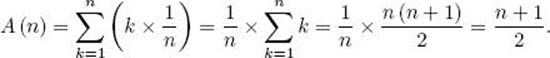
The third step in this quadruple equality is derived in Example A.1 of Appendix A. As we would expect, on the average, about half the array is searched.

Next we analyze the case in which x may not be in the array. To analyze this case we must assign some probability p to the event that x is in the array. If x is in the array, we will again assume that it is equally likely to be in any of the slots from 1 to n. The probability that x is in the kth slot is thenp/n, and the probability that it is not in the array is 1 − p. Recall that there are k passes through the loop if x is found in the kth slot, and n passes through the loop if x is not in the array. The average time complexity is therefore given by

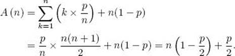
The last step in this triple equality is derived with algebraic manipulations. If p = 1, A(n) = (n + 1)/2, as before, whereas if p = 1/2, A(n) = 3n/4 + 1/4. This means that about 3/4 of the array is searched on the average.

Before proceeding, we offer a word of caution about the average. Although an average is often referred to as a typical occurrence, one must be careful in interpreting the average in this manner. For example, a meteorologist may say that a typical January 25 in Chicago has a high of 22^◦ F because 22^◦ F has been the average high for that date over the past 80 years. The paper may run an article saying that the typical family in Evanston, Illinois earns $50,000 annually because that is the average income. An average can be called “typical” only if the actual cases do not deviate much from the average (that is, only if the standard deviation is small). This may be the case for the high temperature on January 25. However, Evanston is a community with families of diverse incomes. It is more typical for a family to make either $20,000 annually or $100,000 annually than to make $50,000. Recall in the previous analysis that A(n) is (n + 1)/2 when it is known that x is in the array. This is not the typical search time, because all search times between 1 and n are equally typical. Such considerations are important in algorithms that deal with response time. For example, consider a system that monitors a nuclear power plant. If even a single instance has a bad response time, the results could be catastrophic. It is therefore important to know whether the average response time is 3 seconds because all response times are around 3 seconds or because most are 1 second and some are 60 seconds.

A final type of time complexity analysis is the determination of the smallest number of times the basic operation is done. For a given algorithm, B(n) is defined as the minimum number of times the algorithm will ever do its basic operation for an input size of n. So B(n) is called the best-case time complexity of the algorithm, and the determination of B(n) is called a best-case time complexity analysis. As is the case for W(n) and A(n), if T(n) exists, then B(n) = T(n). Let’s determine B(n) for Algorithm 1.1.

Analysis of Algorithm 1.1

Best-Case Time Complexity (Sequential Search)

Basic operation: the comparison of an item in the array with x.

Input size: n, the number of items in the array.

Because n ≥ 1, there must be at least one pass through the loop, If x = S[1], there will be one pass through the loop regardless of the size of n. Therefore,

For algorithms that do not have every-case time complexities, we do worst-case and average-case analyses much more often than best-case analyses. An average-case analysis is valuable because it tells us how much time the algorithm would take when used many times on many different inputs. This would be useful, for example, in the case of a sorting algorithm that was used repeatedly to sort all possible inputs. Often, a relatively slow sort can occasionally be tolerated if, on the average, the sorting time is good. In Section 2.4 we will see an algorithm, named Quicksort, that does exactly this. It is one of the most popular sorting algorithms. As noted previously, an average-case analysis would not suffice in a system that monitored a nuclear power plant. In this case, a worst-case analysis would be more useful because it would give us an upper bound on the time taken by the algorithm. For both the applications just discussed, a best-case analysis would be of little value.

We have discussed only the analysis of the time complexity of an algorithm. All the same considerations just discussed also pertain to analysis of memory complexity, which is an analysis of how efficient the algorithm is in terms of memory. Although most of the analyses in this text are time complexity analyses, we will occasionally find it useful to do a memory complexity analysis.

In general, a complexity function can be any function that maps the positive integers to the nonnegative reals. When not referring to the time complexity or memory complexity for some particular algorithm, we will usually use standard function notation, such as f(n) and g(n), to represent complexity functions.

Example 1.6

The functions

are all examples of complexity functions because they all map the positive integers to the nonnegative reals.

• 1.3.2 Applying the Theory

When applying the theory of algorithm analysis, one must sometimes be aware of the time it takes to execute the basic operation, the overhead instructions, and the control instructions on the actual computer on which the algorithm is implemented. By “overhead instructions” we mean instructions such as initialization instructions before a loop. The number of times these instructions execute does not increase with input size. By “control instructions” we mean instructions such as incrementing an index to control a loop. The number of times these instructions execute increases with input size. The basic operation, overhead instructions, and control instructions are all properties of an algorithm and the implementation of the algorithm. They are not properties of a problem. This means that they are usually different for two different algorithms for the same problem.

Suppose we have two algorithms for the same problem with the following every-case time complexities: n for the first algorithm and n² for the second algorithm. The first algorithm appears more efficient. Suppose, however, a given computer takes 1,000 times as long to process the basic operation once in the first algorithm as it takes to process the basic operation once in the second algorithm. By “process” we mean that we are including the time it takes to execute the control instructions. Therefore, if t is the time required to process the basic operation once in the second algorithm, 1,000t is the time required to process the basic operation once in the first algorithm. For simplicity, let’s assume that the time it takes to execute the overhead instructions is negligible in both algorithms. This means the times it takes the computer to process an instance of size n are n × 1,000t for the first algorithm and n² × t for the second algorithm. We must solve the following inequality to determine when the first algorithm is more efficient:

Dividing both sides by nt yields

If the application never had an input size larger than 1,000, the second algorithm should be implemented. Before proceeding, we should point out that it is not always so easy to determine precisely when one algorithm is faster than another. Sometimes we must use approximation techniques to analyze the inequalities obtained by comparing two algorithms.

Recall that we are assuming that the time it takes to process the overhead instructions is negligible. If this were not the case, these instructions would also have to be considered to determine when the first algorithm would be more efficient.

• 1.3.3 Analysis of Correctness

In this text, “analysis of an algorithm” means an efficiency analysis in terms of either time or memory. There are other types of analyses. For example, we can analyze the correctness of an algorithm by developing a proof that the algorithm actually does what it is supposed to do. Although we will often informally show that our algorithms are correct and will sometimes prove that they are, you should see Dijkstra (1976), Gries (1981), or Kingston (1990) for a comprehensive treatment of correctness.

1.4 Order

We just illustrated that an algorithm with a time complexity of n is more efficient than one with a time complexity of n² for sufficiently large values of n, regardless of how long it takes to process the basic operations in the two algorithms. Suppose now that we have two algorithms for the same problem and that their every-case time complexities are 100n for the first algorithm and 0.01n² for the second algorithm. Using an argument such as the one just given, we can show that the first algorithm will eventually be more efficient than the second one. For example, if it takes the same amount of time to process the basic operations in both algorithms and the overhead is about the same, the first algorithm will be more efficient if

Dividing both sides by 0.01n yields

If it takes longer to process the basic operation in the first algorithm than in the second, then there is simply some larger value of n at which the first algorithm becomes more efficient.

Algorithms with time complexities such as n and 100n are called linear-time algorithms because their time complexities are linear in the input size n, whereas algorithms with time complexities such as n² and 0.01n² are called quadratic-time algorithms because their time complexities are quadratic in the input size n. There is a fundamental principle here. That is, any linear-time algorithm is eventually more efficient than any quadratic-time algorithm. In the theoretical analysis of an algorithm, we are interested in eventual behavior. Next we will show how algorithms can be grouped according to their eventual behavior. In this way we can readily determine whether one algorithm’s eventual behavior is better than another’s.

• 1.4.1 An Intuitive Introduction to Order

Functions such as 5n² and 5n² + 100 are called pure quadratic functions because they contain no linear term, whereas a function such as 0.1n² + n + 100 is called a complete quadratic function because it contains a linear term. Table 1.3 shows that eventually the quadratic term dominates this function. That is, the values of the other terms eventually become insignificant compared with the value of the quadratic term. Therefore, although the function is not a pure quadratic function, we can classify it with the pure quadratic functions. This means that if some algorithm has this time complexity, we can call the algorithm a quadratic-time algorithm. Intuitively, it seems that we should always be able to throw away low-order terms when classifying complexity functions. For example, it seems that we should be able to classify 0.1n³ + 10n² + 5n + 25 with pure cubic functions. We will soon establish rigorously that we can do this. First let’s try to gain an intuitive feel for how complexity functions are classified.

The set of all complexity functions that can be classified with pure quadratic functions is called Θ(n²), where Θ is the Greek capital letter “theta.” If a function is a member of the set Θ(n²), we say that the function is order of n². For example, because we can throw away low-order terms,

which means that g(n) is order of n². As a more concrete example, recall from Section 1.3.1 that the time complexity for Algorithm 1.3 (Exchange Sort) is given by T(n) = n(n − 1)/2. Because

throwing away the lower-order term n/2 shows that T(n) ∈ Θ(n²).

• Table 1.3 The quadratic term eventually dominates

When an algorithm’s time complexity is in Θ(n²), the algorithm is called a quadratic-time algorithm or a Θ(n²) algorithm. We also say that the algorithm is Θ(n²). Exchange Sort is a quadratic-time algorithm.

Similarly, the set of complexity functions that can be classified with pure cubic functions is called Θ(n³), and functions in that set are said to be order of n³, and so on. We will call these sets complexity categories. The following are some of the most common complexity categories:

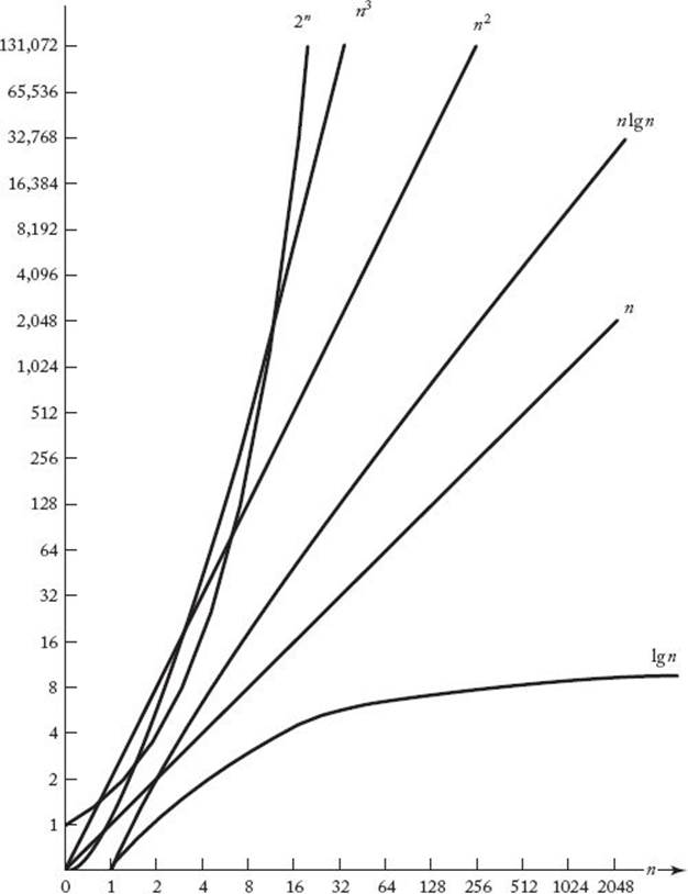
In this ordering, if f(n) is in a category to the left of the category containing g(n), then f(n) eventually lies beneath g(n) on a graph. Figure 1.3 plots the simplest members of these categories: n, ln n, n ln n, and so on. Table 1.4 shows the execution times of algorithms whose time complexities are given by these functions. The simplifying assumption is that it takes 1 nanosecond (10⁻⁹ second) to process the basic operation for each algorithm. The table shows a possibly surprising result. One might expect that as long as an algorithm is not an exponential-time algorithm, it will be adequate. However, even the quadratic-time algorithm takes 31.7 years to process an instance with an input size of 1 billion. On the other hand, the Θ(n ln n) algorithm takes only 29.9 seconds to process such an instance. Ordinarily an algorithm has to be Θ(n ln n) or better for us to assume that it can process extremely large instances in tolerable amounts of time. This is not to say that algorithms whose time complexities are in the higher-order categories are not useful. Algorithms with quadratic, cubic, and even higher-order time complexities can often handle the actual instances that arise in many applications.

Before ending this discussion, we stress that there is more information in knowing a time complexity exactly than in simply knowing its order. For example, recall the hypothetical algorithms, discussed earlier, that have time complexities of 100n and 0.01n². If it takes the same amount of time to process the basic operations and execute the overhead instructions in both algorithms, then the quadratic-time algorithm is more efficient for instances smaller than 10,000. If the application never requires instances larger than this, the quadratic-time algorithm should be implemented. If we knew only that the time complexities were in Θ(n) and Θ(n²), respectively, we would not know this. The coefficients in this example are extreme, and in practice they are often less extreme. Furthermore, there are times when it is quite difficult to determine the time complexities exactly. Therefore, we are sometimes content to determine only the order.

• 1.4.2 A Rigorous Introduction to Order

The previous discussion imparted an intuitive feel for order (Θ). Here we develop theory that enables us to define order rigorously. We accomplish this by presenting two other fundamental concepts. The first is “big O.”

Figure 1.3 Growth rates of some common complexity functions.

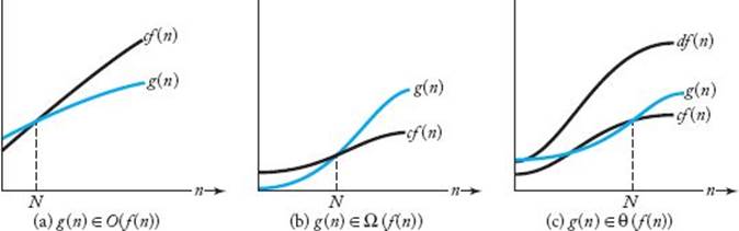
Definition

For a given complexity function f(n), O(f(n)) is the set of complexity functions g(n) for which there exists some positive real constant c and some nonnegative integer N such that for all n ≥ N,

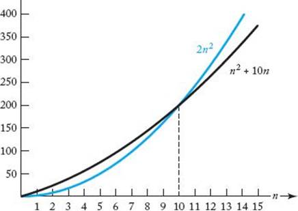
If g(n) ∈ O(f(n)), we say that g(n) is big O of f(n). Figure 1.4(a) illustrates “big O.” Although g(n) starts out above cf(n) in that figure, eventually it falls beneath cf(n) and stays there. Figure 1.5 shows a concrete example. Although n² + 10n is initially above 2n² in that figure, for n ≥ 10

• Table 1.4 Execution times for algorithms with the given time complexities

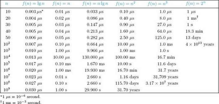
Figure 1.4 Illustrating “big O,” Ω, and Θ.

We can therefore take c = 2 and N = 10 in the definition of “big O” to conclude that

If, for example, g(n) is in O(n²), then eventually g(n) lies beneath some pure quadratic function cn² on a graph. This means that if g(n) is the time complexity for some algorithm, eventually the running time of the algorithm will be at least as fast as quadratic. For the purposes of analysis, we can say that eventually g(n) is at least as good as a pure quadratic function. “Big O” (and other concepts that will be introduced soon) are said to describe the asymptotic behavior of a function because they are concerned only with eventual behavior. We say that “big O” puts an asymptotic upper boundon a function.

Figure 1.5 The function n² + 10n eventually stays beneath the function 2n².

The following examples illustrate how to show “big O.”

Example 1.7

We show that 5n² ∈ O(n²). Because, for n ≥ 0,

we can take c = 5 and N = 0 to obtain our desired result.

Example 1.8

Recall that the time complexity of Algorithm 1.3 (Exchange Sort) is given by

Because, for n ≥ 0,

we can take c = 1/2 and N = 0 to conclude that T(n) ∈ O(n²).

A difficulty students often have with “big O” is that they erroneously think there is some unique c and unique N that must be found to show that one function is “big O” of another. This is not the case at all. Recall that Figure 1.5 illustrates that n² + 10n ∈ O(n²) using c = 2 and N = 10. Alternatively, we could show it as follows.

Example 1.9

We show that n² + 10n ∈ O(n²). Because, for n ≥ 1,

we can take c = 11 and N = 1 to obtain our result.

In general, one can show “big O” using whatever manipulations seem most straightforward.

Example 1.10

We show that n² ∈ O(n² + 10n). Because, for n ≥ 0,

we can take c = 1 and N = 0 to obtain our result.

The purpose of this last example is to show that the function inside “big O” does not have to be one of the simple functions plotted in Figure 1.3. It can be any complexity function. Ordinarily, however, we take it to be a simple function like those plotted in Figure 1.3.

Example 1.11

We show that n ∈ O(n²). Because, for n ≥ 1,

we can take c = 1 and N = 1 to obtain our result.

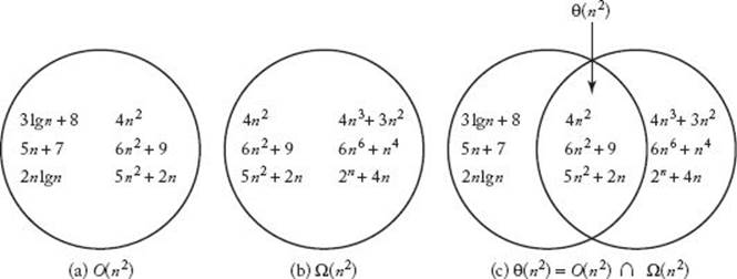
This last example makes a crucial point about “big O.” A complexity function need not have a quadratic term to be in O(n²). It need only eventually lie beneath some pure quadratic function on a graph. Therefore, any logarithmic or linear complexity function is in O(n²). Similarly, any logarithmic, linear, or quadratic complexity function is in O(n³), and so on. Figure 1.6(a) shows some exemplary members of O(n²).

Just as “big O” puts an asymptotic upper bound on a complexity function, the following concept puts an asymptotic lower bound on a complexity function.

Figure 1.6 The sets O(n²), Ω(n²), Θ(n²). Some exemplary members are shown.

Definition

For a given complexity function f(n), Ω(f(n)) is the set of complexity functions g(n) for which there exists some positive real constant c and some nonnegative integer N such that, for all n ≥ N,

The symbol Ω is the Greek capital letter “omega.” If g(n) ∈ Ω(f(n)), we say that g(n) is omega of f(n). Figure 1.4(b) illustrates Ω. Some examples follow.

Example 1.12

We show that 5n² ∈ Ω(n²). Because, for n ≥ 0,

we can take c = 1 and N = 0 to obtain our result.

Example 1.13

We show that n² + 10n ∈ Ω(n²). Because, for n ≥ 0, n² + 10n ≥ n²,

we can take c = 1 and N = 0 to obtain our result.

Example 1.14

Consider again the time complexity of Algorithm 1.3 (Exchange Sort). We show that

For n ≥ 2,

Therefore, for n ≥ 2,

which means we can take c = 1/4 and N = 2 to obtain our result.

As is the case for “big O,” there are no unique constants c and N for which the conditions in the definition of Ω hold. We can choose whichever ones make our manipulations easiest.

If a function is in Ω(n²), then eventually the function lies above some pure quadratic function on a graph. For the purposes of analysis, this means that eventually it is at least as bad as a pure quadratic function. However, as the following example illustrates, the function need not be a quadratic function.

Example 1.15

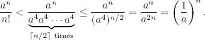
We show that n³ ∈ Ω(n²). Because, if n ≥ 1,

we can take c = 1 and N = 1 to obtain our result.

Figure 1.6(b) shows some exemplary members of Ω(n²)

If a function is in both O(n²) and Ω(n²) we can conclude that eventually the function lies beneath some pure quadratic function on a graph and eventually it lies above some pure quadratic function on a graph. That is, eventually it is at least as good as some pure quadratic function and eventually it is at least as bad as some pure quadratic function. We can therefore conclude that its growth is similar to that of a pure quadratic function. This is precisely the result we want for our rigorous notion of order. We have the following definition.

Definition

For a given complexity function f(n),

This means that Θ(f(n)) is the set of complexity functions g(n) for which there exists some positive real constants c and d and some nonnegative integer N such that, for all n ≥ N,

If g(n) ∈ Θ(f(n)), we say that g(n) is order of f(n).

Example 1.16

Consider once more the time complexity of Algorithm 1.3. Examples 1.8 and 1.14 together establish that

This means that T(n) ∈ O(n²) ∩ Ω(n²) = Θ(n²)

Figure 1.6(c) depicts that Θ(n²) is the intersection of O(n²) and Ω(n²), whereas Figure 1.4(c) illustrates Θ. Notice in Figure 1.6(c) that the function 5n + 7 is not in Ω(n²), and the function 4n³ + 3n² is not in O(n²). Therefore, neither of these functions is in Θ(n²). Although intuitively this seems correct, we have not yet proven it. The following example shows how such a proof proceeds.

Example 1.17

We show that n is not in Ω(n²) by using proof by contradiction. In this type of proof we assume something is true—in this case, that n ∈ Ω(n²)—and then we do manipulations that lead to a result that is not true. That is, the result contradicts something known to be true. We then conclude that what we assumed in the first place cannot be true.

Assuming that n ∈ Ω(n²) means we are assuming that there exists some positive constant c and some nonnegative integer N such that, for n ≥ N,

If we divide both sides of this inequality by cn, we have, for n ≥ N,

However, for any n > 1/c, this inequality cannot hold, which means that it cannot hold for all n ≥ N. This contradiction proves that n is not in Ω(n²).

We have one more definition concerning order that expresses relationships such as the one between the function n and the function Ω(n²).

Definition

For a given complexity function f(n), o(f(n)) is the set of all complexity functions g(n) satisfying the following: For every positive real constant c there exists a nonnegative integer N such that, for all n ≥ N,

If g(n) ∈ o(f(n)), we say that g(n) is small o of f(n). Recall that “big O” means there must be some real positive constant c for which the bound holds. This definition says that the bound must hold for every real positive constant c. Because the bound holds for every positive c, it holds for arbitrarily small c. For example, if g(n) ∈ o(f(n)), there is an N such that, for n > N,

We see that g(n) becomes insignificant relative to f(n) as n becomes large. For the purposes of analysis, if g(n) is in o(f(n)), then g(n) is eventually much better than functions such as f(n). The following examples illustrate this.

Example 1.18

We show that

Let c > 0 be given. We need to find an N such that, for n ≥ N,

If we divide both sides of this inequality by cn, we get

Therefore, it suffices to choose any N ≥ 1/c.

Notice that the value of N depends on the constant c. For example, if c = 0.00001, we must take N equal to at least 100,000. That is, for

Example 1.19

We show that n is not in o(5n). We will use proof by contradiction to show this. If n ∈ o(5n), then there must exist some N such that, for n ≥ N,

This contradiction proves that n is not in o(5n).

The following theorem relates “small o” to our other asymptotic notation.

Theorem 1.2

If g(n) ∈ o(f(n)), then

That is, g(n) is in O(f(n)) but is not in Ω(f(n)).

Proof: Because g(n) ∈ o(f(n)), for every positive real constant c there exists an N such that, for all n ≥ N,

which means that the bound certainly holds for some c. Therefore,

We will show that g(n) is not in Ω(f (n)) using proof by contradiction. If g(n) ∈ Ω(f(n)), then there exists some real constant c > 0 and some N₁ such that, for all n ≥ N₁,

But, because g(n) ∈ o(f(n)), there exists some N₂ such that, for all n ≥ N₂,

Both inequalities would have to hold for all n greater than both N₁ and N₂. This contradiction proves that g(n) cannot be in Ω(f(n)).

You may think that o(f(n)) and O(f(n))−Ω(f(n)) must be the same set. This is not true. There are unusual functions that are in O(f(n)) − Ω(f(n)) but that are not in o(f(n)). The following example illustrates this.

Example 1.20

Consider the function

It is left as an exercise to show that

Example 1.20, of course, is quite contrived. When complexity functions represent the time complexities of actual algorithms, ordinarily the functions in O(f(n)) − Ω(f(n)) are the same ones that are in o(f(n)).

Let’s discuss Θ further. In the exercises we establish that

For example,

This means that Θ separates complexity functions into disjoint sets. We will call these sets complexity categories. Any function from a given category can represent the category. For convenience, we ordinarily represent a category by its simplest member. The previous complexity category is represented by Θ(n²).

The time complexities of some algorithms do not increase with n. For example, recall that the best-case time complexity B(n) for Algorithm 1.1 is 1 for every value of n. The complexity category containing such functions can be represented by any constant, and for simplicity we represent it by Θ(1).

The following are some important properties of order that make it easy to determine the orders of many complexity functions. They are stated without proof. The proofs of some will be derived in the exercises, whereas the proofs of others follow from results obtained in the next subsection. The second result we have already discussed. It is included here for completeness.

Properties of Order:

This implies that all logarithmic complexity functions are in the same complexity category. We will represent this category by Θ(lg n).

4. If b > a > 0, then

This implies that all exponential complexity functions are not in the same complexity category.

5. For all a > 0

This implies that n! is worse than any exponential complexity function.

6. Consider the following ordering of complexity categories:

where k > j > 2 and b > a > 1. If a complexity function g(n) is in a category that is to the left of the category containing f(n), then

7. If c ≥ 0, d > 0, g(n) ∈ O(f(n)), and h(n) ∈ Θ(f(n)), then

Example 1.21

Property 3 states that all logarithmic complexity functions are in the same complexity category. For example,

This means that the relationship between log₄ n and lg n is the same as the one between 7n² + 5n and n².

Example 1.22

Property 6 states that any logarithmic function is eventually better than any polynomial, any polynomial is eventually better than any exponential function, and any exponential function is eventually better than the factorial function. For example,

Example 1.23

Properties 6 and 7 can be used repeatedly. For example, we can show that 5n + 3 lg n + 10n lg n + 7n² ∈ Θ(n²), as follows. Repeatedly applying Properties 6 and 7, we have

which means

which means

which means

In practice, we do not repeatedly appeal to the properties, but rather we simply realize that we can throw out low-order terms.

If we can obtain the exact time complexity of an algorithm, we can determine its order simply by throwing out low-order terms. When this is not possible, we can appeal back to the definitions of “big O” and Ω to determine order. For example, suppose for some algorithm we are unable to determine T(n) [or W(n), A(n), or B(n)] exactly. If we can show that

by appealing directly to the definitions, we can conclude that T(n) ∈ Θ(f(n)).

Sometimes it is fairly easy to show that T(n) ∈ O(f(n)) but difficult to determine whether T(n) is in Ω(f (n)). In such cases we may be content to show only that T(n) ∈ O(f(n)), because this implies that T(n) is at least as good as functions such as f(n). Similarly, we may be content to learn only thatT(n) ∈ Ω(f(n)), because this implies that T(n) is at least as bad as functions such as f(n).

Before closing, we mention that many authors say

Both mean the same thing—namely, that f(n) is a member of the set Θ(n²). Similarly, it is common to write

You are referred to Knuth (1973) for an account of the history of “order” and to Brassard (1985) for a discussion of the definitions of order given here. Our definitions of “big O,” Ω, and Θ are, for the most part, standard. There are, however, other definitions of “small o.” It is not standard to call the sets Θ(n), Θ(n²), and so on, “complexity categories.” Some authors call them “complexity classes,” although this term is used more often to refer to the sets of problems discussed in Chapter 9. Other authors do not give them any particular name at all.

• 1.4.3 Using a Limit to Determine Order

We now show how order can sometimes be determined using a limit. This material is included for those familiar with limits and derivatives. Knowledge of this material is not required elsewhere in the text.

Theorem 1.3

We have the following:

Proof: The proof is left as an exercise.

Example 1.24

Theorem 1.3 implies that

because

Using Theorem 1.3 in Example 1.24 is not very exciting because the result could have easily been established directly. The following examples are more interesting.

Example 1.25

Theorem 1.3 implies that, for b > a > 0,

because

The limit is 0 because 0 < a/b < 1.

This is Property 4 in the Properties of Order (near the end of Section 1.4.2).

Example 1.26

Theorem 1.3 implies that, for a > 0,

If a ≤ 1, the result is trivial. Suppose that a > 1. If n is so large that

then

Because a > 1, this implies that

This is Property 5 in the Properties of Order.

The following theorem, whose proof can be found in most calculus texts, enhances the usefulness of Theorem 1.3.

Theorem 1.4

L’Hôpital’s Rule If f(x) and g(x) are both differentiable with derivatives f′(x) and g′(x), respectively, and if

then

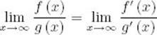
whenever the limit on the right exists.

Theorem 1.4 holds for functions of real valuables, whereas our complexity functions are functions of integer variables. However, most of our complexity functions (for example, lg n, n, etc.) are also functions of real variables. Furthermore, if a function f(x) is a function of a real variable x, then

where n is an integer, whenever the limit on the right exists. Therefore, we can apply Theorem 1.4 to complexity analysis, as the following examples illustrate.

Example 1.27

Theorems 1.3 and 1.4 imply that

because

Example 1.28

Theorems 1.3 and 1.4 imply that, for b > 1 and a > 1,

because

This is Property 3 in the Properties of Order.

1.5 Outline of This Book

We are now ready to develop and analyze sophisticated algorithms. For the most part, our organization is by technique rather than by application area. As noted earlier, the purpose of this organization is to establish a repertoire of techniques that can be investigated as possible ways to approach a new problem. Chapter 2 discusses a technique called “divide-and-conquer.” Chapter 3 covers dynamic programming. Chapter 4 addresses “the greedy approach.” In Chapter 5, the backtracking technique is presented. Chapter 6 discusses a technique related to backtracking called “branch-and-bound.” In Chapters 7 and 8, we switch from developing and analyzing algorithms to analyzing problems themselves. Such an analysis, which is called a computational complexity analysis, involves determining a lower bound for the time complexities of all algorithms for a given problem. Chapter 7 analyzes the Sorting Problem, and Chapter 8 analyzes the Searching Problem. Chapter 9 is devoted to a special class of problems. That class contains problems for which no one has ever developed an algorithm whose time complexity is better than exponential in the worst case. Yet no one has ever proven that such an algorithm is not possible. It turns out that there are thousands of such problems and that they are all closely related. The study of these problems has become a relatively new and exciting area of computer science. In Chapter 10 we revert back to developing algorithms. However, unlike the methods presented in Chapters 2–6, we discuss algorithms for solving a certain type of problem. That is, we discuss number-theoretic algorithms, which are algorithms that solve problems involving the integers. All of the algorithms discussed in the first nine chapters are developed for a computer containing a single processor that executes a single sequence of instructions. Owing to the drastic reduction in the price of computer hardware, there has been a recent increase in the development of parallel computers. Such computers have more than one processor, and all the processors can execute instructions simultaneously (in parallel). Algorithms written for such computers are called “parallel algorithms.” Chapter 11 is an introduction to such algorithms.

EXERCISES

Sections 1.1

1. Write an algorithm that finds the largest number in a list (an array) of n numbers.

2. Write an algorithm that finds the m smallest numbers in a list of n numbers.

3. Write an algorithm that prints out all the subsets of three elements of a set of n elements. The elements of this set are stored in a list that is the input to the algorithm.

4. Write an Insertion Sort algorithm (Insertion Sort is discussed in Section 7.2) that uses Binary Search to find the position where the next insertion should take place.

5. Write an algorithm that finds the greatest common divisor of two integers.

6. Write an algorithm that finds both the smallest and largest numbers in a list of n numbers. Try to find a method that does at most 1.5n comparisons of array items.

7. Write an algorithm that determines whether or not an almost complete binary tree is a heap.

Sections 1.2

8. Under what circumstances, when a searching operation is needed, would Sequential Search (Algorithm 1.1) not be appropriate?

9. Give a practical example in which you would not use Exchange Sort (Algorithm 1.3) to do a sorting task.

Sections 1.3

10. Define basic operations for your algorithms in Exercises 1–7, and study the performance of these algorithms. If a given algorithm has an every-case time complexity, determine it. Otherwise, determine the worst-case time complexity.

11. Determine the worst-case, average-case, and best-case time complexities for the basic Insertion Sort and for the version given in Exercise 4, which uses Binary Search.

12. Write a Θ(n) algorithm that sorts n distinct integers, ranging in size between 1 and kn inclusive, where k is a constant positive integer. (Hint: Use a knelement array.)

13. Algorithm A performs 10n² basic operations, and algorithm B performs 300 ln n basic operations. For what value of n does algorithm B start to show its better performance?

14. There are two algorithms called Alg1 and Alg2 for a problem of size n. Alg1 runs in n² microseconds and Alg2 runs in 100n log n microseconds. Alg1 can be implemented using 4 hours of programmer time and needs 2 minutes of CPU time. On the other hand, Alg2 requires 15 hours of programmer time and 6 minutes of CPU time. If programmers are paid 20 dollars per hour and CPU time costs 50 dollars per minute, how many times must a problem instance of size 500 be solved using Alg2 in order to justify its development cost?

Sections 1.4

15 Show directly that f(n) = n² + 3n³ ∈ Θ(n³). That is, use the definitions of O and Ω to show that f(n) is in both O(n³) and Ω(n³).

16. Using the definitions of O and Ω, show that

17. Using the Properties of Order in Section 1.4.2, show that

18. Let p(n) = a_kn^k + a_k−1n^k−1 + · · · + a₁n + a₀, where a_k > 0. Using the Properties of Order in Section 1.4.2, show that p(n) ∈ Θ(n^k).

19. The function f(x) = 3n² +10n log n+1000n+4 log n+9999 belongs in which of the following complexity categories:

(a) θ(lg n)

(b) θ(n² log n)

(c) θ(n)

(d) θ(n lg n)

(e) θ(n²)

(f) None of these

20. The function f(x) = (log n)² + 2n + 4n + log n + 50 belongs in which of the following complexity categories:

(a) θ(lg n)

(b) θ((log n)²)

(c) θ(n)

(d) θ(n lg n)

(e) θ(n(lg n)²)

(f) None of these

21. The function f(x) = n + n² + 2ⁿ + n⁴ belongs in which of the following complexity categories:

(a) θ(n)

(b) θ(n²)

(c) θ(n³)

(d) θ(n lg n)

(e) θ(n⁴)

(f) None of these

22. Group the following functions by complexity category.

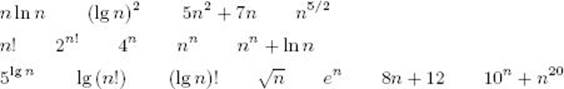
23. Establish Properties 1, 2, 6, and 7 of the Properties of Order in Section 1.4.2.

24. Discuss the reflexive, symmetric, and transitive properties for asymptotic comparisons (O, Ω, Θ, o).

25. Suppose you have a computer that requires 1 minute to solve problem instances of size n = 1,000. Suppose you buy a new computer that runs 1,000 times faster than the old one. What instance sizes can be run in 1 minute, assuming the following time complexities T(n) for our algorithm?

(a) T(n) = n

(b) T(n) = n³

(c) T(n) = 10ⁿ

26. Derive the proof of Theorem 1.3.

27. Show the correctness of the following statements.

(a) lg n ∈ O (n)

(b) n ∈ O (n lg n)

(c) n lg n ∈ O(n²)

(d) 2ⁿ ∈ Ω _5ln n

(e) lg³ n ∈ (n^0.5)

Additional Exercises

28. Presently we can solve problem instances of size 30 in 1 minute using algorithm A, which is a Θ(2ⁿ) algorithm. On the other hand, we will soon have to solve problem instances twice this large in 1 minute. Do you think it would help to buy a faster (and more expensive) computer?

29. Consider the following algorithm:

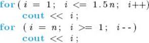
(a) What is the output when n = 2, n = 4, and n = 6?

(b) What is the time complexity T(n)? You may assume that the input n is divisible by 2.

30. Consider the following algorithm:

(a) What is the output when n = 6, n = 8, and n = 10?

(b) What is the time complexity T(n)? You may assume that the input n is divisible by 2.

31. Consider the following algorithm:

(a) What is the output when n = 4, n = 16, n = 32?

(b) What is the time complexity T(n). You may assume that n is divisible 4.

32. What is the time complexity T(n) of the nested loops below? For simplicity, you may assume that n is a power of 2. That is, n = 2^k for some positive integer k.

33. Give an algorithm for the following problem and determine its time complexity. Given a list of n distinct positive integers, partition the list into two sublists, each of size n/2, such that the difference between the sums of the integers in the two sublists is maximized. You may assume that n is a multiple of 2.

34. What is the time complexity T(n) of the nested loops below? For simplicity, you may assume that n is a power of 2. That is, n = 2^k for some positive integer k.

35. Consider the following algorithm:

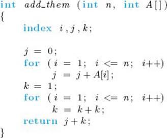
(a) If n = 5 and the array A contains 2, 5, 3, 7, and 8, what is the output?

(b) What is the time complexity T(n) of the algorithm?

(c) Try to improve the efficiency of the algorithm.

36. Consider the following algorithm:

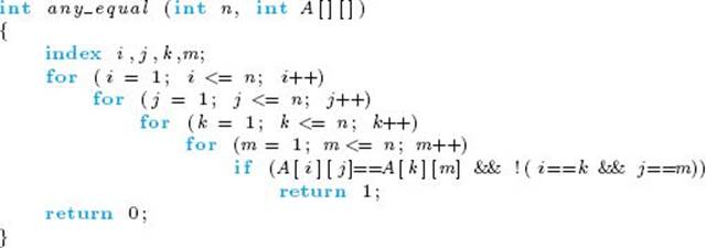
(a) What is the best case time complexity of the algorithm (assuming n > 1)?

(b) What is the worst case time complexity of the algorithm?

(c) Try to improve the efficiency of the algorithm.

(d) What property holds for the array A if the algorithm returns 0?

(e) What property holds for the array A if the algorithm returns 1?

37. Give a Θ(lg n) algorithm that computes the remainder when xⁿ is divided by p. For simplicity, you may assume that n is a power of 2. That is, n = 2^k for some positive integer k.

38. Explain in English what functions are in the following sets.

(a) n^O(1)

(b)

(c)

39. Show that the function f (n) = | n² = sin n| is in neither O(n) nor Ω(n).

40. Justify the correctness of the following statements assuming that f(n) and g(n) are asymptotically positive functions.

(a) f (n) + g (n) ∈ O (max (f (n)) , g (n))

(b) f²(n) ∈ Ω(f(n))

(c) f(n) + o(f(n)) ∈ Θ(f(n)), where o(f(n)) means any function g(n) ∈ o(f(n))

41. Give an algorithm for the following problem. Given a list of n distinct positive integers, partition the list into two sublists, each of size n/2, such that the difference between the sums of the integers in the two sublists is minimized. Determine the time complexity of your algorithm. You may assume that n is a multiple of 2.

42. Algorithm 1.7 (nth Fibonacci Term, Iterative) is clearly linear in n, but is it a linear-time algorithm? In Section 1.3.1 we defined the input size as the size of the input. In the case of the nth Fibonacci term, n is the input, and the number of bits it takes to encode n could be used as the input size. Using this measure, the size of 64 is lg 64 = 6, and the size of 1,024 is lg 1,024 = 10. Show that Algorithm 1.7 is exponential-time in terms of its input size. Show further that any algorithm for computing the nth Fibonacci term must be an exponential-time algorithm because the size of the output is exponential in the input size. (See Section 9.2 for a related discussion of the input size.)

43. Determine the time complexity of Algorithm 1.6 (nth Fibonacci Term, Recursive) in terms of its input size (see Exercise 34).

44. Can you verify the correctness of your algorithms for Exercises 1 to 7?