Foundations of Algorithms (2015)

Chapter 12 Introduction to Parallel Algorithms

Suppose you want to build a fence in your backyard and it’s necessary to dig 10 deep holes, one for each fence post. Realizing that it would be a laborious and unpleasant task to individually dig the 10 holes in sequence, you look for some alternative. You remember how Mark Twain’s famous character Tom Sawyer tricked his friends into helping him whitewash a fence by pretending it was fun. You decide to use the same clever ruse, but you update it a bit. You pass out flyers to your health-conscious neighbors announcing a hole-digging contest in your backyard. Whoever is most fit should be able to dig a hole fastest and therefore win the contest. You offer some insignificant first prize, such as a six-pack of beer, knowing that the prize is not really important to your neighbors. Rather, they just want to prove how fit they are. On contest day, 10 strong neighbors simultaneously dig 10 holes. This is called digging the holes in parallel. You have saved yourself a lot of work and completed the hole digging much faster than you would have done by digging them in sequence by yourself.

Just as you can complete the hole-digging job faster by having friends work in parallel, often a computer can complete a job faster if it has many processors executing instructions in parallel. (A processor in a computer is a hardware component that processes instructions and data.) So far we have discussed only sequential processing. That is, all of the algorithms we’ve presented have been designed to be implemented on a traditional sequential computer. Such a computer has one processor executing instructions in sequence, similar to your digging the 10 holes in sequence by yourself. These computers are based on the model introduced by John von Neumann. As Figure 12.1 illustrates, this model consists of a single processor, called the central processing unit (CPU), and memory. The model takes a single sequence of instructions and operates on a single sequence of data. Such a computer is called a single instruction stream, single data stream (SISD) computer, and is popularly known as a serial computer.

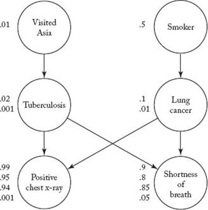
Many problems could be solved much faster if a computer had many processors executing instructions simultaneously (in parallel). This would be like having your 10 neighbors dig the 10 holes at the same time. For example, consider the Bayesian network introduced in Section 6.3. Figure 12.2shows such a network. Each vertex in that network represents a possible condition of a patient. There is an edge from one vertex to another if having the condition at the first vertex could cause one to have the condition at the second vertex. For example, the top-right vertex represents the condition of being a smoker, and the edge emanating from that vertex means that smoking can cause lung cancer. A given cause does not always result in its potential effects. Therefore, the probability of each effect given each of its causes also needs to be stored in the network. For example, the probability (0.5) of being a smoker is stored at the vertex containing “Smoker.” The probability (0.1) of having lung cancer, given that one is a smoker, and the probability (0.01) of having lung cancer, given that one is not a smoker, are stored at the vertex containing “Lung cancer.” The probability (0.99) of having a positive chest x-ray, given that one has both tuberculosis and lung cancer, along with the probabilities of having a positive chest x-ray, given the other three combinations of values of its causes, are stored at the vertex containing “Positive chest x-ray.” The basic inference problem in a Bayesian network is to determine the probability of having the conditions at all remaining vertices when it is learned that the conditions at certain vertices are present. For example, if a patient was known to be a smoker and to have had a positive chest x-ray, we might want to know the probabilities that the patient had lung cancer, had tuberculosis, had shortness of breath, and had recently visited Asia. Pearl (1986) developed an inference algorithm for solving this problem. In this algorithm, each vertex sends messages to its parents and children. For example, when it is learned that the patient has a positive chest x-ray, the vertex for “Positive chest x-ray” sends messages to its parents “Tuberculosis” and “Lung cancer.” When each of these vertices receives its message, the probability of the condition at the vertex is computed, and the vertex then sends messages to its parents and other children. When these vertices receive messages, the new probabilities of the conditions at the vertices are computed, and the vertices then send messages. The message-passing scheme terminates at roots and leaves. When it is learned that the patient is also a smoker, another message stream begins at that vertex. A traditional sequential computer can compute the value of only one message or one probability at a time. The value of the message to “Tuberculosis” could be computed first, then the new probability of tuberculosis, then the value of the message to “Lung cancer,” then its probability, and so on.

Figure 12.1 A traditional serial computer.

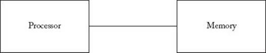
Figure 12.2 A Bayesian network.

If each vertex had its own processor that was capable of sending messages to the processors at the other vertices, when it is learned that the patient has a positive chest x-ray, we could first compute and send the messages to “Tuberculosis” and “Lung cancer.” When each of these vertices received its message, it could independently compute and send messages to its parents and other children. Furthermore, if we also know that the patient was a smoker, the vertex containing “Smoker” could simultaneously be computing and sending a message to its child. Clearly, if all this were taking place simultaneously, the inference could be done much more quickly. A Bayesian network used in actual applications often contains hundreds of vertices, and the inferred probabilities are needed immediately. This means that the time savings could be quite significant.

What we have just described is an architecture for a particular kind of parallel computer. Such computers are called “parallel” because each processor can execute instructions simultaneously (in parallel) with all the other processors. The cost of processors has decreased dramatically over the past three decades. Currently, the speed of an off-the-shelf microprocessor is within one order of magnitude of the speed of the fastest serial computer. However, microprocessors cost many orders of magnitude less. Therefore, by connecting microprocessors as described in the previous paragraph, it is possible to obtain computing power faster than the fastest serial computer for substantially less money. There are many applications that can benefit significantly from parallel computation. Applications in artificial intelligence include the Bayesian Network problem described previously, inference in neural networks, natural language understanding, speech recognition, and machine vision. Other applications include database query processing, weather prediction, pollution monitoring, analysis of protein structures, and many more.

There are many ways to design parallel computers. Section 12.1 discusses some of the considerations necessary in parallel design and some of the most popular parallel architectures. Section 12.2 shows how to write algorithms for one particular kind of parallel computer, called a PRAM (for “parallel random access machine”). As we shall see, this particular kind of computer is not very practical. However, the PRAM model is a straightforward generalization of the sequential model of computation. Furthermore, a PRAM algorithm can be translated into algorithms for many practical machines. So PRAM algorithms serve as a good introduction to parallel algorithms.

12.1 Parallel Architectures

The construction of parallel computers can vary in each of the following three ways:

1. Control mechanism

2. Address-space organization

3. Interconnection network

• 12.1.1 Control Mechanism

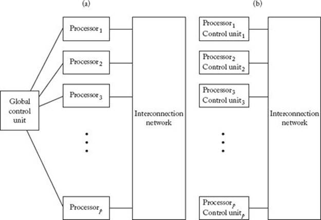
Each processor in a parallel computer can operate either under the control of a centralized control unit or independently under the control of its own control unit. The first kind of architecture is called single instruction stream, multiple data stream (SIMD). Figure 12.3(a) illustrates an SIMD architecture. The interconnection network depicted in the figure represents the hardware that enables the processors to communicate with each other. Interconnection networks are discussed in Section 12.1.3. In an SIMD architecture, the same instruction is executed synchronously by all processing units under the control of the central control unit. Not all processors must execute an instruction in each cycle; any given processor can be switched off in any given cycle.

Parallel computers, in which each processor has its own control unit, are called multiple instruction stream, multiple data stream (MIMD) computers. Figure 12.3(b) illustrates an MIMD architecture. MIMD computers store both the operating system and the program at each processor.

SMID computers are suited for programs in which the same set of instructions is executed on different elements of a data set. Such programs are called data parallel programs. A drawback of SIMD computers is that they cannot execute different instructions in the same cycle. For example, suppose the following conditional statement is being executed:

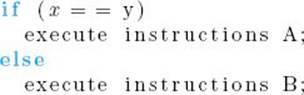
Figure 12.3 (a) A single instruction stream, multiple data stream (SIMD) architecture. (b) A multiple instruction stream, multiple data stream (MIMD) architecture.

Any processor that finds x ≠ y (recall that the processors are processing different data elements) must do nothing while the processors that find x = y are executing instructions A. Those that find x = y must then be idle while the others are executing instructions B.

In general, SIMD computers are best suited to parallel algorithms that require synchronization. Many MIMD computers have extra hardware that provides synchronization, which means that they can emulate SIMD computers.

• 12.1.2 Address-Space Organization

Processors can communicate with each other either by modifying data in a common address space or by passing messages. The address space is organized differently according to the communication method used.

Shared-Address-Space Architecture

In a shared-address-space architecture, the hardware provides for read and write access by all processors to a shared address space. Processors communicate by modifying data in the shared address space. Figure 12.4(a) depicts a shared-address-space architecture in which the time it takes each processor to access any word in memory is the same. Such a computer is called a uniform memory access (UMA) computer. In a UMA computer, each processor may have its own private memory, as shown in Figure 12.4(a). This private memory is used only to hold local variables necessary for the processor to carry out its computations. None of the actual input to the algorithm is in the private area. A drawback of a UMA computer is that the interconnection network must simultaneously provide access for every processor to the shared memory. This can significantly slow down performance. Another alternative is to provide each processor with a portion of the shared memory. This is illustrated in Figure 12.4(b). This memory is not private, as is the local memory in Figure 12.4(a). That is, each processor has access to the memory stored at another processor. However, it has faster access to its own memory than to memory stored at another processor. If most of a processor’s accesses are to its own memory, performance should be good. Such a computer is called a nonuniform memory access (NUMA) computer.

Figure 12.4 (a) A uniform memory access (UMA) computer. (b) A nonuniform memory access (NUMA) computer.

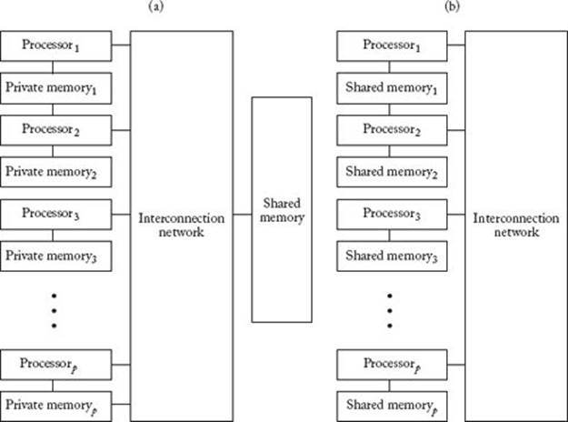
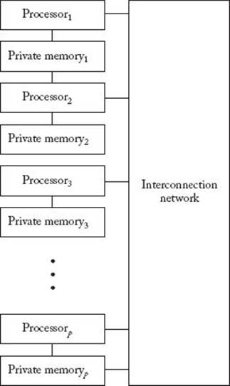
Message-Passing Architecture

In a message-passing architecture, each processor has its own private memory that is accessible only to that processor. Processors communicate by passing messages to other processors rather than by modifying data elements. Figure 12.5 shows a message-passing architecture. Notice that Figure 12.5 looks much like Figure 12.4(b). The difference is in the way in which the interconnection network is wired. In the case of the NUMA computer, the interconnection network is wired to allow each processor access to the memory stored at the other processors, whereas in the message-passing computer it is wired to allow each processor to send a message directly to each of the other processors.

Figure 12.5 A message-passing architecture. Each processor’s memory is accessible only to that processor. Processors communicate by passing messages to each other through the interconnection network.

• 12.1.3 Interconnection Networks

There are two general categories of interconnection networks: static and dynamic. Static networks are typically used to construct message-passing architectures, whereas dynamic networks are typically used to construct shared-address-space architectures. We discuss each of these types of networks in turn.

Static Interconnection Networks

A static interconnection network contains direct links between processors and are sometimes called direct networks. There are several different types of static interconnection networks. Let’s discuss some of the most common ones. The most efficient, but also the most costly, is a completely connected network, which is illustrated in Figure 12.6(a). In such a network, every processor is directly linked to every other processor. Therefore, a processor can send a message to another processor directly on the link to that processor. Because the number of links is quadratic in terms of the number of processors, this type of network is quite costly.

In a star-connected network, one processor acts as the central processor. That is, every other processor has a link only to that processor. Figure 12.6(b) depicts a star-connected network. In a star-connected network, a processor sends a message to another processor by sending the message to the central processor, which in turn routes the message to the receiving processor.

Figure 12.6 (a) A completely connected network. (b) A star-connected network. (c) A bounded-degree network of degree 4.

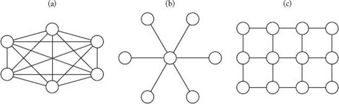
In a bounded-degree network of degree d, each processor is linked to at most d other processors. Figure 12.6(c) shows a bounded-degree network of degree 4. In a bounded-degree network of degree 4, a message can be passed by sending it first along one direction and then along the other direction until it reaches its destination.

A slightly more complex, but popular, static network is the hypercube. A zero-dimensional hypercube consists of a single processor. A one-dimensional hypercube is formed by linking the processors in two zero-dimensional hypercubes. A two-dimensional hypercube is formed by linking each processor in a one-dimensional hypercube to one processor in another one-dimensional hypercube. Recursively, a (d + 1)-dimensional hypercube is formed by linking each processor in a d-dimensional hypercube to one processor in another d-dimensional hypercube. A given processor in the first hypercube is linked to the processor occupying the corresponding position in the second hypercube. Figure 12.7 illustrates hypercube networks.

It should be clear that the reason why static networks are ordinarily used to implement message-passing architectures is that the processors in such networks are directly linked, enabling the flow of messages.

Dynamic Interconnection Networks

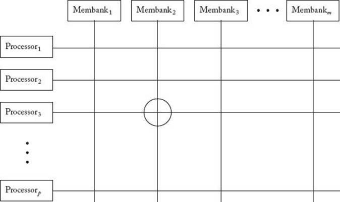
In a dynamic interconnection network, processors are connected to memory through a set of switching elements. One of the most straightforward ways to do this is to use a crossbar switching network. In such a network, p processors are connected to m memory banks using a grid of switching elements, as shown in Figure 12.8. If, for example, processor₃ can currently access membank₂, the switch at the grid position circled in Figure 12.8 is closed (closing the switch completes the circuit, enabling the flow of electricity). This network is called “dynamic” because the connection between a processor and a memory bank is made dynamically when a switch is closed. A crossbar switching network is nonblocking. That is, the connection of one processor to a given memory bank does not block the connection of another processor to another memory bank. Ideally, in a crossbar switching network there should be a bank for every word in memory. However, this is clearly impractical. Ordinarily, the number of banks is at least as large as the number of processors, so that, at a given time, every processor is capable of accessing at least one memory bank. The number of switches in a crossbar switching network is equal to pm. Therefore, if we require that m be greater than or equal to p, the number of switches is greater than or equal to p². As a result, crossbar switching networks can become quite costly when the number of processors is large.

Figure 12.7 Hypercube networks.

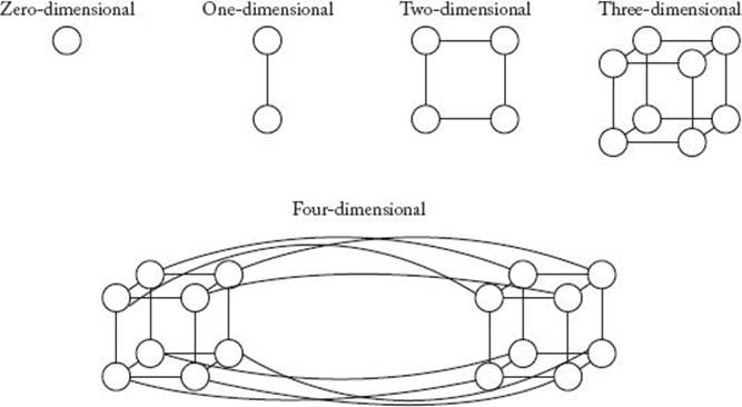
Figure 12.8 A crossbar switching network. There is a switch at every position on the grid. The circled switch is closed, enabling the flow of information between processor₃ and membank₂, when the third processor is currently allowed to access the second memory bank.

Other dynamic interconnection networks, which will not be discussed here, include bus-based networks and multistage interconnection networks.

It should be clear why dynamic interconnection networks are ordinarily used to implement shared-address-space architectures. That is, in such networks each processor is allowed to access every word in memory but cannot send a direct message to any of the other processors.

The introduction to parallel hardware presented here is based largely on the discussion in Kumar, Grama, Gupta, and Karypis (1994). The reader is referred to that text for a more thorough introduction and, in particular, for a discussion of bus-based and multistage interconnection networks.

12.2 The PRAM Model

As discussed in the preceding section, quite a few different parallel architectures are possible, and computers have actually been manufactured with many of these architectures. All serial computers, on the other hand, have the architecture shown in Figure 12.1, which means that the von Neumann model is a universal model for all serial computers. The only assumption that was made in designing the algorithms in the previous chapters was that they would run on a computer conforming to the von Neumann model. Therefore, each of these algorithms has the same time complexity regardless of the programming language or computer used to implement the algorithm. This has been a key factor in the impressive growth of the application of serial computers.

It would be useful to find a universal model for parallel computation. Any such model must first be sufficiently general to capture the key features of a large class of parallel architectures. Second, algorithms designed according to this model must execute efficiently on actual parallel computers. No such model is currently known, and it seems unlikely that one will be found.

Although no universal model is currently known, the parallel random access machine (PRAM) computer has become widely used as a theoretical model for parallel machines. A PRAM computer consists of p processors, all of which have uniform access to a large shared memory. Processors share a common clock but may execute different instructions in each cycle. Therefore, a PRAM computer is a synchronous, MIMD, UMA computer. This means that Figures 12.3(b) and 12.4(a) depict the architecture of a PRAM computer, whereas Figure 12.8 shows a possible interconnection network for such a machine. As already noted, it would be quite costly to actually construct such a computer. However, the PRAM model is a natural extension of the serial model of computation. This makes the PRAM model conceptually easy to work with when developing algorithms. Furthermore, algorithms developed for the PRAM model can be translated into algorithms for many of the more practical computers. For example, a PRAM instruction can be simulated in Θ(lg p) instructions on a bounded-degree network, where p is the number of processors. Additionally, for a large class of problems, PRAM algorithms are asymptotically as fast as algorithms for a hypercube. For these reasons, the PRAM model serves as a good introduction to parallel algorithms.

In a shared-memory computer such as a PRAM, more than one processor can try to read from or write to the same memory location simultaneously. There are four versions of the PRAM model depending on how concurrent memory accesses are handled.

1. Exclusive-read, exclusive-write (EREW). In this version, no concurrent reads or writes are allowed. That is, only one processor can access a given memory location at a given time. This is the weakest version of the PRAM computer, because it allows minimal concurrency.

2. Exclusive-read, concurrent-write (ERCW). In this version, simultaneous write operations are allowed, but not simultaneous read operations.

3. Concurrent-read, exclusive-write (CREW). In this version, simultaneous read operations are allowed, but not simultaneous write operations.

4. Concurrent-read, concurrent-write (CRCW). In this version, both simultaneous read and write operations are allowed.

We discuss algorithmic design for the CREW PRAM model and the CRCW PRAM model. First we address the CREW model, then we show how more efficient algorithms can sometimes be developed using the CRCW model. Before proceeding, let’s discuss how we present parallel algorithms. Although programming languages for parallel algorithms exist, we will use our standard pseudocode with some additional features, which will be described next.

Just one version of the algorithm is written, and after compilation it is executed by all processors simultaneously. Therefore, each processor needs to know its own index while executing the algorithm. We will assume that the processors are indexed P₁, P₂, P₃, etc., and that the instruction

p = index of this processor;

returns the index of a processor. A variable declared in the algorithm could be a variable in shared memory, which means that it is accessible to all processors, or it could be in private memory (see Figure 12.4a). In this latter case, each processor has its own copy of the variable. We use the key word local when declaring a variable of this type.

All our algorithms will be data-parallel algorithms, as discussed in Section 12.1.1. That is, the processors will execute the same set of instructions on different elements of a data set. The data set will be stored in shared memory. If an instruction assigns the value of an element of this data set to a local variable, we call this a read from shared memory, whereas if it assigns the value of a local variable to an element of this data set, we call this a write to shared memory. The only instructions we use for manipulating elements of this data set are reads from and writes into shared memory. For example, we never directly compare the values of two elements of the data set. Rather, we read their values into variables in local memory and then compare the values of those variables. We will allow direct comparisons to variables like n, the size of the data set. A data-parallel algorithm consists of a sequence of steps, and every processor starts each step at the same time and ends each step at the same time. Furthermore, all processors that read during a given step read at the same time, and all processors that write during a given step write at the same time.

Finally, we assume that as many processors as we want are always available to us. In practice, as already noted, this is often an unrealistic assumption.

The following algorithm illustrates these conventions. We are assuming that there is an array of integers S, indexed from 1 to n, in shared memory and that n processors, indexed from 1 to n, are executing the algorithm in parallel.

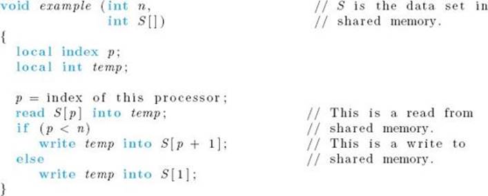
All of the values in the array S are read into n different local variables temp simultaneously. Then the values in the n variables temp are all written back out to S simultaneously. Effectively, every element in S is given the value of its predecessor (with wraparound). Figure 12.9 illustrates the operation of the algorithm. Notice that each processor always has access to the entire array S because S is in shared memory. So the pth processor can write to the (p + 1)st array slot.

There is only one step in this simple algorithm. When there is more than one step, we write loops such as the following:

Figure 12.9 Application of procedure example.

There are various ways this loop can be implemented. One way is to have a separate control unit do the incrementing and testing. It would issue instructions telling the other processors when to read, when to execute instructions on local variables, and when to write. Inside the loop, we sometimes do calculations on a variable that always has the same value for all processors. For example, Algorithms 12.1 and 12.3 both execute the instruction

where size has the same value for all processors. To make it clear that each processor does not need its own copy of such a variable, we will declare the variable as a variable in shared memory. The instruction can be implemented by having a separate control unit execute it. We won’t discuss implementation further. Rather, we proceed to writing algorithms.

• 12.2.1 Designing Algorithms for the CREW PRAM Model

We illustrate CREW PRAM algorithms with the following exemplary problems.

Finding the Largest Key in an Array

Theorem 8.7 proves that it takes at least n − 1 comparisons to find the largest key only by comparisons of keys, which means that any algorithm for the problem, designed to run on a serial computer, must be Θ(n). Using parallel computation, we can improve on this running time. The parallelalgorithm still must do at least n − 1 comparisons. But by doing many of them in parallel, it finishes sooner. We develop this algorithm next.

Recall that Algorithm 8.2 (Find Largest Key) finds the largest key in optimal time as follows:

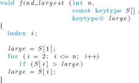
This algorithm cannot benefit from using more processors because the result of each iteration of the loop is needed for the next iteration. Recall from Section 8.5.3 the Tournament method for finding the largest key. This method pairs the numbers into groups of two and finds the largest (winner) of each pair. Then it pairs the winners and finds the largest of each of these pairs. It continues until only one key remains. Figure 8.10 illustrates this method. A sequential algorithm for the Tournament method has the same time complexity as Algorithm 8.2. However, this method can benefit from using more processors. For example, suppose you wish to find the largest of eight keys using this method. You have to determine each of four winners in the first round in sequence before proceeding to the second round. If you have the help of three friends, each of you can simultaneously determine one of the winners of the first round. This means that the first round can be completed four times as fast. After that round, two of you can rest while the other two perform the comparisons in the second round. In the final round, only one of you needs to do a comparison.

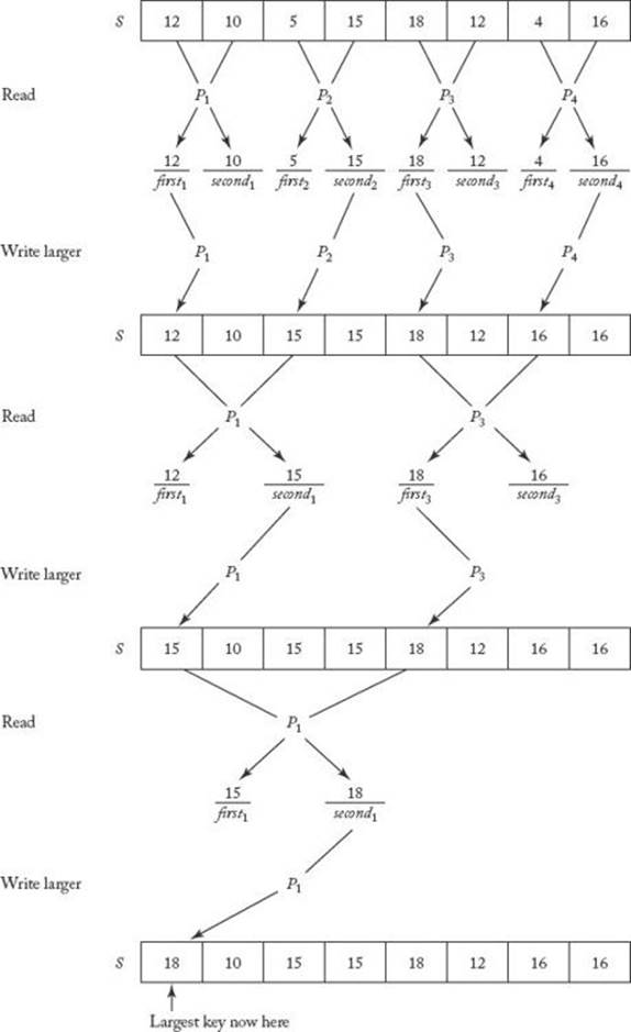
Figure 12.10 illustrates how a parallel algorithm for this method proceeds. We need only half as many processors as array elements. Each processor reads two array elements into local variables first and second. It then writes the larger of first and second into the first of the array slots from which it has read. After three such rounds, the largest key ends up in S [1]. Each round is a step in the algorithm. In the example shown in Figure 12.10, n = 8 and there are lg 8 = 3 steps. Algorithm 12.1 is an algorithm for the actions illustrated in Figure 12.10. Notice that this algorithm is written as a function. When a parallel algorithm is written as a function, it is necessary that at least one processor return a value and that all processors that do return values return the same value.

Figure 12.10 Use of parallel processors to implement the Tournament method for finding the largest key.

Algorithm 12.1

Parallel Find Largest Key

Problem: Find the largest key in an array S of size n.

Inputs: positive integer n, array of keys S indexed from 1 to n.

Outputs: the value of the largest key in S.

Comment: It is assumed that n is a power of 2 and that we have n/2 processors executing the algorithm in parallel. The processors are indexed from 1 to n/2 and the command “index of this processor” returns the index of a processor.

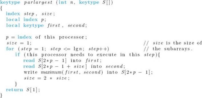
We used the high-level pseudocode “if (this processor needs to execute in this step)” in order to keep the algorithm as lucid as possible. In Figure 12.10 we see that the processors used in a given step are the ones for which

for some integer k (notice that size doubles in value in each step). Therefore, the actual check of whether the processor should execute is

Alternatively, we can simply allow all the processors to execute in each step. The ones that need not execute simply do useless comparisons. For example, in the second round, processor P₂ compares the value of S [3] with the value of S [5] and writes the larger value into S [3]. Even though this isunnecessary, P₂ may as well be doing it because nothing is gained by keeping P₂ idle. The important things are that the processors that should be executing are executing and that the other processors are not changing the values of memory locations needed by the ones that should be executing. The only problem presented by allowing unneeded processors to execute instructions is that sometimes they end up referring to array elements outside the range of S. For example, in the previous algorithm, P₄ refers to S [9] in the second round. This can be handled by simply padding S with additional slots. We end up wasting space this way, but we save time by eliminating the check of whether the processor should be executing.

When analyzing a parallel algorithm, we do not analyze the total amount of work done by the algorithm. Rather, we analyze the total amount of work done by any one processor because this gives us a good idea of how fast the computer will process the input. Because each processor does about lg n passes through the for-step loop in Algorithm 12.1, we have

This is a substantial improvement over the sequential algorithm.

Applications of Dynamic Programming

Many dynamic programming applications are amenable to parallel design because often the entries in a given row or diagonal can all be computed simultaneously. We illustrate this approach by rewriting the algorithm for the binomial coefficient (Algorithm 3.2) as a parallel algorithm. In this algorithm, the entries in a given row of Pascal’s triangle (see Figure 3.1) are computed in parallel.

Algorithm 12.2

Parallel Binomial Coefficient

Problem: Compute the binomial coefficient.

Inputs: nonnegative integers n and k, where k ≤ n.

Outputs: the binomial coefficient .

Comment: It is assumed that we have k + 1 processors executing the algorithm in parallel. The processors are indexed from 0 to k, and the command “index of this processor” returns the index of a processor.

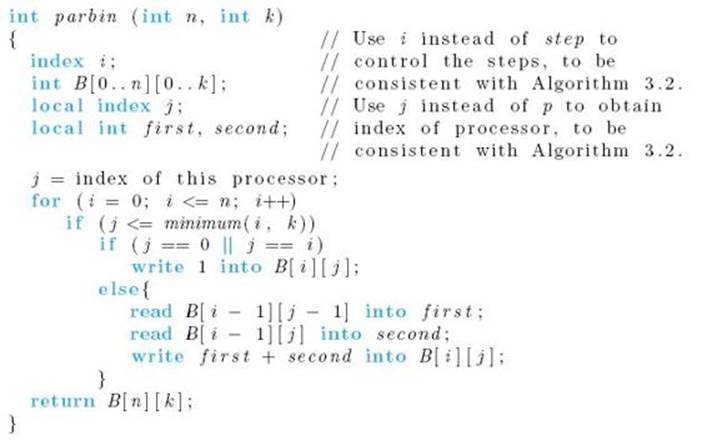
The control statement in Algorithm 3.2

is replaced in this algorithm by the control statement

because all k processors execute in each pass through the for-i loop. Instead of sequentially computing the values of B [i] [j] with j ranging from 0 to minimum (i, k), the parallel algorithm has the processors that are indexed from 0 to minimum (i, k) simultaneously computing the values.

Clearly, there are n + 1 passes through a loop in our parallel algorithm. Recall that there are Θ(nk) passes through a loop in the sequential algorithm (Algorithm 3.2).

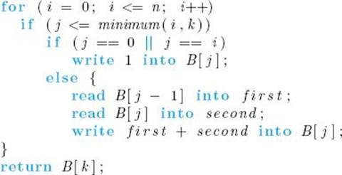
Recall from Exercise 3.4 that it is possible to implement Algorithm 3.2 using only a one-dimensional array B that is indexed from 0 to k. This modification is very straightforward in the case of the parallel algorithm, because on entry to the ith pass through the for-i loop the entire (i − 1)st row of Pascal’s triangle can be read from B into the k local pairs of variables first and second. Then, on exit, the entire ith row can be written into B. The pseudocode is as follows:

Parallel Sorting

Recall the dynamic programming version of Mergesort 3 (Algorithm 7.3). That algorithm simply starts with the keys as singletons, merges pairs of keys into sorted lists containing two keys, merges pairs of those lists into sorted lists containing four keys, and so on. That is, it does the merging depicted in Figure 2.2. This is very similar to using the Tournament method to find the maximum. That is, we can do the merging at each step in parallel. The following algorithm implements this method. Again, for simplicity, it is assumed that n is a power of 2. When this is not the case, the array size can be treated as a power of 2, but merging is not done beyond n. The dynamic programming version of Mergesort 3 (Algorithm 7.3) shows how to do this.

Algorithm 12.3

Parallel Mergesort

Problem: Sort n keys in nondecreasing order.

Inputs: positive integer n, array of keys S indexed from 1 to n.

Outputs: the array S containing the keys in nondecreasing order.

Comment: It is assumed that n is a power of 2 and that we have n/2 processors executing the algorithm in parallel. The processors are indexed from 1 to n/2, and the command “index of this processor” returns the index of a processor.

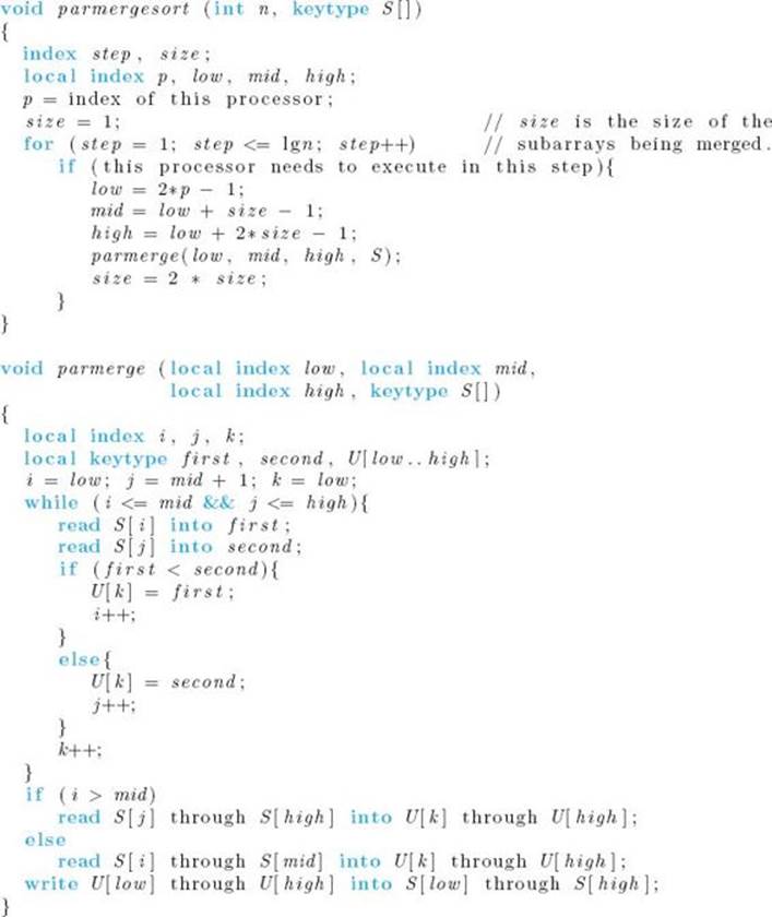
The check of whether a processor should execute in a given step is the same as the check in Algorithm 12.1. That is, we need to do the following check:

Recall that we can reduce the number of assignments of records in the single-processor iterative version of Mergesort (Algorithm 7.3) by reversing the roles of U and S in each pass through the for loop. That same improvement can be done here. If this were done, U would have to be an array, indexed from 1 to n, in shared memory. We present the basic version of parmerge for the sake of simplicity.

The time complexity of this algorithm is not obvious. Therefore, we do a formal analysis.

Analysis of Algorithm 12.3

Worst-Case Time Complexity

Basic operation: the comparison that takes place in parmerge.

Input size: n, the number of keys in the array.

This algorithm does exactly the same number of comparisons as does the ordinary sequential Mergesort. The difference is that many of them are done in parallel. In the first pass through the for-step loop, n/2 pairs of arrays, each containing only one key, are merged simultaneously. So the worst-case number of comparisons done by any processor is 2 − 1 = 1 (see the analysis of Algorithm 2.3 in Section 2.2). In the second pass, n/4 pairs of arrays, each containing two keys, are merged simultaneously. So the worst-case number of comparisons is 4−1 = 3. In the third pass, n/8 pairs of arrays, each containing four keys, are merged simultaneously. So the worst-case number of comparisons is 8 − 1 = 7. In general, in the ith pass, n/2ⁱ pairs of arrays, each containing 2ⁱ⁻¹ keys, are merged simultaneously, and the worst-case number of comparisons is 2ⁱ − 1. Finally, in the last pass, two arrays, each containing n/2 keys, are merged, which means that the worst-case number of comparisons in this pass is n − 1. The total worst-case number of comparisons done by each processor is given by

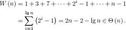
The last equality is derived from the result in Example A.3 in Appendix A and some algebraic manipulations.

We have successfully done parallel sorting by comparisons of keys in linear time, which is a significant improvement over the Θ(n lg n) required by sequential sorting. It is possible to improve our parallel merging algorithm so that parallel mergesorting is done in time. This improvement is discussed in the exercises. Even this is not optimal, because parallel sorting can be done in Θ(lg n) time. See Kumar, Grama, Gupta, and Karypis (1994) or Akl (1985) for a thorough discussion of parallel sorting.

• 12.2.2 Designing Algorithms for the CRCW PRAM Model

Recall that CRCW stands for concurrent-read, concurrent-write. Unlike concurrent reads, concurrent writes must somehow be resolved when two processors try to write to the same memory location in the same step. The most frequently used protocols for resolving such conflicts are as follows:

• Common. This protocol allows concurrent writes only if all the processors are attempting to write the same values.

• Arbitrary. This protocol picks an arbitrary processor as the one allowed to write to the memory location.

• Priority. In this protocol, all the processors are organized in a predefined priority list, and only the one with the highest priority is allowed to write.

• Sum. This protocol writes the sum of the quantities being written by the processors. (This protocol can be extended to any associative operator defined on the quantities being written.)

Figure 12.11 Application of Algorithm 12.4. Only T [3] ends up equal to 1, because S [3] is the largest key and therefore is the only key never to lose a comparison.

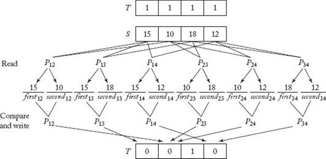
We write an algorithm for finding the largest key in an array that works with common-write, arbitrary-write, and priority-write protocols and that is faster than the one given previously for the CREW model (Algorithm 12.1). The algorithm proceeds as follows. Let the n keys be in an array S in shared memory. We maintain a second array T of n integers in shared memory, and initialize all elements in T to 1. Next we assume that we have n (n − 1)/2 processors indexed as follows:

In parallel, we have all the processors compare S [i] with S [j]. In this way, every element in S is compared with every other element in S. Each processor writes a 0 into T [i] if S [i] loses the comparison and a 0 into T [j] if S [j] loses. Only the largest key never loses a comparison. Therefore, the only element of T that remains equal to 1 is the one that is indexed by k such that S [k] contains the largest key. So the algorithm need only return the value of S [k] such that T [k] = 1. Figure 12.11 illustrates these steps, and the algorithm follows. Notice in the algorithm that when more than one processor writes to the same memory location, they all write the same value. This means that the algorithm works with common-write, arbitrary-write, and priority-write protocols.

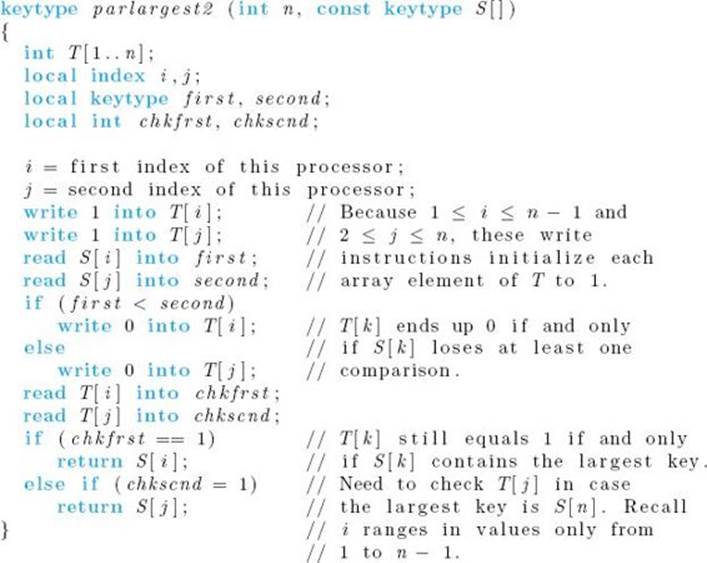
Algorithm 12.4

Parallel CRCW Find Largest Key

Problem: Find the largest key in an array S of n keys.

Inputs: positive integer n, array of keys S indexed from 1 to n.

Outputs: the value of the largest key in S.

Comment: It is assumed that n is a power of 2 and that we have n (n − 1)/2 processors executing the algorithm in parallel. The processors are indexed as

and the command “first index of this processor” returns the value of i, whereas the command “second index of this processor” returns j.

There is no loop in this algorithm, which means that it finds the largest key in constant time. This is quite impressive, because it means that we could find the largest of 1,000,000 keys in the same amount of time required to find the largest of only 10 keys. However, this optimal time complexity has been bought at the expense of quadratic-time processor complexity. We would need about 1,000,000²/2 processors to find the largest of 1,000,000 keys.

This chapter has served only as a brief introduction to parallel algorithms. A thorough introduction requires a text of its own. One such text is Kumar, Grama, Gupta, and Karypis (1994).

EXERCISES

Section 12.1

1. If we assume that one person can add two numbers in t_a time, how long will it take that person to add two n × n matrices, if we consider the operation of addition as the basic operation? Justify your answer.

2. If we have two people add numbers and it takes t_a time for one person to add two numbers, how long will the two people take to add two n × n matrices, if we consider the operation of addition as the basic operation? Justify your answer.

3. Consider the problem of adding two n × n matrices. If it takes t_a time for one person to add two numbers, how many people do we need to minimize the total time spent to get the final answer? What will be the minimum amount of time needed to find the answer, if we assume that we have enough people? Justify your answers.

4. Assuming that one person can add two numbers in t_a time, how long will it take that person to add all n numbers of a list, if we consider the operation of addition as the basic operation? Justify your answer.

5. If we have two people add n numbers in a list and it takes t_a time for one person to add two numbers, how long will it take the two people to add all n numbers in the list, if we consider the operation of addition as the basic operation and include t_p time for passing the result of an addition from one person to the other? Justify your answer.

6. Consider the problem of adding n numbers in a list. If it takes t_a time for one person to add two numbers and it takes no time to pass the result of an addition from one person to another, how many people do we need to minimize the total time spent to get the final answer? What will be the minimum amount of time needed to find the answer, if we assume we have enough people? Justify your answer.

Section 12.2

7. Write a CREW PRAM algorithm for adding all n numbers in a list in Θ(lg n) time.

8. Write a CREW PRAM algorithm that uses n² processors to multiply two n × n matrices. Your algorithm should perform better than the standard Θ(n³)-time serial algorithm.

9. Write a PRAM algorithm for Quicksort using n processors to sort a list of n elements.

10. Write a sequential algorithm that implements the Tournament method to find the largest key in an array of n keys. Show that this algorithm is no more efficient than the standard sequential algorithm.

11. Write a PRAM algorithm using n³ processors to multiply two n×n matrices. Your algorithm should run in Θ(lg n) time.

12. Write a PRAM algorithm for the Shortest Paths problem of Section 3.2. Compare the performance of your algorithm against the performance of Floyd’s algorithm (Algorithm 3.3).

13. Write a PRAM algorithm for the Chained Matrix Multiplication problem of Section 3.4. Compare the performance of your algorithm against the performance of the Minimum Multiplications algorithm (Algorithm 3.6).

14. Write a PRAM algorithm for the Optimal Binary Search Tree problem of Section 3.5. Compare the performance of your algorithm against the performance of the Optimal Binary Search Tree algorithm (Algorithm 3.9).

Additional Exercises

15. Consider the problem of adding the numbers in a list of n numbers. If it takes t_a (n − 1) time for one person to add all n numbers, is it possible for m people to compute the sum in less than [t_a (n − 1)] /m time? Justify your answer.

16. Write a PRAM algorithm that runs in Θ((_lg n)²) time for the problem of mergesorting. (Hint: Use n processors, and assign each processor to a key to determine the position of the key in the final list by binary searching.)

17. Write a PRAM algorithm for the Traveling Salesperson problem of Section 3.6. Compare the performance of your algorithm against the performance of the Traveling Salesperson algorithm (Algorithm 3.11).