Foundations of Algorithms (2015)
Appendix B Solving Recurrence Equations: With Applications to Analysis of Recursive Algorithms
The analysis of recursive algorithms is not as straightforward as it is for iterative algorithms. Ordinarily, however, it is not difficult to represent the time complexity of a recursive algorithm by a recurrence equation. The recurrence equation must then be solved to determine the time complexity. We discuss techniques for solving such equations and for using the solutions in the analysis of recursive algorithms.
B.1 Solving Recurrences Using Induction
Mathematical induction is reviewed in Appendix A. Here we show how it can be used to analyze some recursive algorithms. We consider first a recursive algorithm that computes n!.
Algorithm B.1
Factorial
Problem: Determine n! = n (n − 1) (n − 2) · · · (3) (2) (1) when n ≥ 1.
0! = 1
Inputs: a nonnegative integer n.
Outputs: n!.
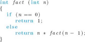
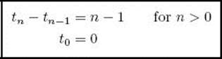
To gain insight into the efficiency of this algorithm, let’s determine how many times this function does the multiplication instruction for each value of n. For a given n, the number of multiplications done is the number done when fact (n − 1) is computed plus the one multiplication done when n is multiplied by fact (n − 1). If we represent the number of multiplications done for a given value of n by tn, we have established that
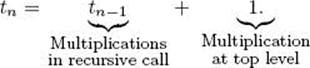
An equation such as this is called a recurrence equation because the value of the function at n is given in terms of the value of the function at a smaller value of n. A recurrence by itself does not represent a unique function. We must also have a starting point, which is called an initial condition. In this algorithm, no multiplications are done when n = 0. Therefore, the initial condition is
![]()
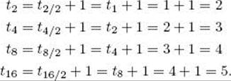
We can compute tn for larger values of n as follows:
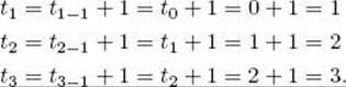
Continuing in this manner gives us more and more values of tn, but it does not enable us to compute tn, for an arbitrary n without starting at 0. We need an explicit expression for tn. Such an expression is called a solution to the recurrence equation. Recall that it is not possible to find a solution using induction. Induction can only verify that a candidate solution is correct. (Constructive induction, which is discussed in Section 8.5.4, can help us discover a solution.) We can obtain a candidate solution to this recurrence by inspecting the first few values. An inspection of the values just computed indicates that
![]()
is the solution. Now that we have a candidate solution, we can use induction to try to prove that it is correct.
Induction base: For n = 0,
![]()
Induction hypothesis: Assume, for an arbitrary positive integer n, that
![]()
Induction step: We need to show that
![]()
If we insert n + 1 in the recurrence, we get
![]()
This completes the induction proof that our candidate solution tn is correct. Notice that we highlight the terms that are equal by the induction hypothesis. We often do this in induction proofs to show where the induction hypothesis is being applied.
There are two steps in the analysis of a recursive algorithm. The first step is determining the recurrence; the second step is solving it. Our purpose here is to show how to solve recurrences. Determining the recurrences for the recursive algorithms in this text is done when we discuss the algorithms. Therefore, in the remainder of this appendix we do not discuss algorithms; rather, we simply take the recurrences as given. We now present more examples of solving recurrences using induction.
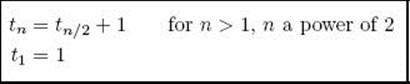
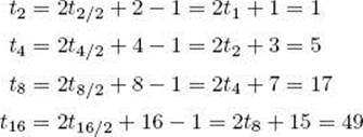
Example B.1
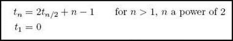
Consider the recurrence
The first few values are
It appears that
![]()
We use induction to prove that this is correct.
Induction base: For n = 1,
![]()
Induction hypothesis: Assume, for an arbitrary n > 0 and n a power of 2, that
![]()
Induction step: Because the recurrence is only for powers of 2, the next value to consider after n is 2n. Therefore, we need to show that
![]()
If we insert 2n in the recurrence, we get
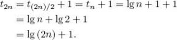
Example B.2
Consider the recurrence
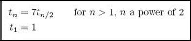
The first few values are
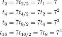
It appears that
![]()
We use induction to prove that this is correct.
Induction base: For n = 1,
![]()
Induction hypothesis: Assume, for an arbitrary n > 0 and n a power of 2, that
![]()
Induction step: We need to show that
![]()
If we insert 2n in the recurrence, we get
![]()
This completes the induction proof. Finally, because
![]()
the solution to this recurrence is usually given as
![]()
Example B.3
Consider the recurrence
The first few values are
There is no obvious candidate solution suggested by these values. As mentioned earlier, induction can only verify that a solution is correct. Because we have no candidate solution, we cannot use induction to solve this recurrence. However, it can be solved using the technique discussed in the next section.
B.2 Solving Recurrences Using the Characteristic Equation
We develop a technique for determining the solutions to a large class of recurrences.
• B.2.1 Homogeneous Linear Recurrences
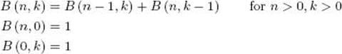
Definition
A recurrence of the form
![]()
where k and the ai terms are constants, is called a homogeneous linear recurrence equation with constant coefficients.
Such a recurrence is called “linear” because every term ti appears only to the first power. That is, there are no terms such as t2n−i, tn−itn−j, and so on. However, there is the additional requirement that there be no terms tc(n−i), where c is a positive constant other than 1. For example, there may not be terms such as tn/2, t3(n−4), etc. Such a recurrence is called “homogeneous” because the linear combination of the terms is equal to 0.
Example B.4
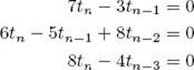
The following are homogeneous linear recurrence equations with constant coefficients:
Example B.5
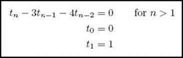
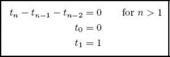
The Fibonacci sequence, which is discussed in Subsection 1.2.2, is defined as follows:
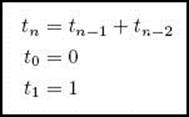
If we subtract tn−1 and tn−2 from both sides, we get
![]()
which shows that the Fibonacci sequence is defined by a homogeneous linear recurrence.
Next we show how to solve a homogeneous linear recurrence.
Example B.6
Suppose we have the recurrence
Notice that if we set
![]()
then
![]()
Therefore, tn = rn is a solution to the recurrence if r is a root of
![]()
Because
![]()
the roots are r = 0, and the roots of
![]()
These roots can be found by factoring:
![]()
The roots are r = 3 and r = 2. Therefore,
![]()
are all solutions to the recurrence. We verify this for 3n by substituting it into the left side of the recurrence, as follows:
With this substitution, the left side becomes
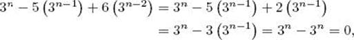
which means that 3n is a solution to the recurrence.
We have found three solutions to the recurrence, but we have more solutions, because if 3n and 2n are solutions, then so is
![]()
where c1 and c2 are arbitrary constants. This result is obtained in the exercises. Although we do not show it here, it is possible to show that these are the only solutions. This expression is therefore the general solution to the recurrence. (By taking c1 = c2 = 0, the trivial solution tn = 0 is included in this general solution.) We have an infinite number of solutions, but which one is the answer to our problem? This is determined by the initial conditions. Recall that we had the initial conditions
![]()
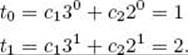
These two conditions determine unique values of c1 and c2 as follows. If we apply the general solution to each of them, we get the following two equations in two unknowns:
These two equations simplify to
![]()
The solution to this system of equations is c1 = 1 and c2 = −1. Therefore, the solution to our recurrence is
![]()
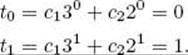
If we had different initial conditions in the preceding example, we would get a different solution. A recurrence actually represents a class of functions, one for each different assignment of initial conditions. Let’s see what function we get if we use the initial conditions
![]()
with the recurrence given in Example B.6. Applying the general solution in Example B.6 to each of these conditions yields
These two equations simplify to
![]()
The solution to this system is c1 = 0 and c2 = 1. Therefore, the solution to the recurrence with these initial conditions is
![]()
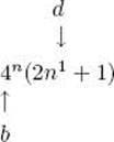
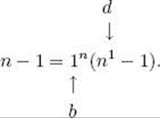
Equation B.1 in Example B.6 is called the characteristic equation for the recurrence. In general, this equation is defined as follows.
Definition
The characteristic equation for the homogeneous linear recurrence equation with constant coefficients
![]()
is defined as
![]()
The value of r0 is simply 1. We write the term as r0 to show the relationship between the characteristic equation and the recurrence.
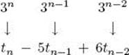
Example B.7
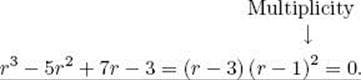
The characteristic equation for the recurrence appears below it:
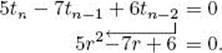
We use an arrow to show that the order of the characteristic equation is k (in this case, 2).
The steps used to obtain the solution in Example B.6 can be generalized into a theorem. To solve a homogeneous linear recurrence with constant coefficients, we need only refer to the theorem. The theorem follows, and its proof appears near the end of this appendix.
![]() Theorem B.1
Theorem B.1
Let the homogeneous linear recurrence equation with constant coefficients
![]()
be given. If its characteristic equation
![]()
has k distinct solutions r1, r2,…, rk, then the only solutions to the recurrence are
![]()
where the ci terms are arbitrary constants.
The values of the k constants ci are determined by the initial conditions. We need k initial conditions to uniquely determine k constants. The method for determining the values of the constants is demonstrated in the following examples.
Example B.8
We solve the recurrence
1. Obtain the characteristic equation:
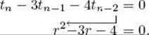
2. Solve the characteristic equation:
![]()
The roots are r = 4 and r = −1.
3. Apply Theorem B.1 to get the general solution to the recurrence:
![]()
4. Determine the values of the constants by applying the general solution to the initial conditions:
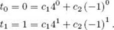
These values simplify to
![]()
The solution to this system is c1 = 1/5 and c2 = −1/5.
5. Substitute the constants into the general solution to obtain the particular solution:
![]()
Example B.9
We solve the recurrence that generates the Fibonacci sequence:
1. Obtain the characteristic equation:
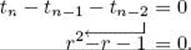
2. Solve the characteristic equation:
From the formula for the solution to a quadratic equation, the roots of this characteristic equation are
![]()
3. Apply Theorem B.1 to get the general solution to the recurrence:
4. Determine the values of the constants by applying the general solution to the initial conditions:
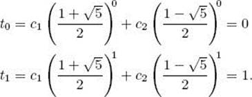
These equations simplify to
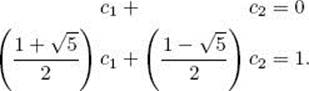
Solving this system yields c1 = 1/√5 and c2 = −1/√5.
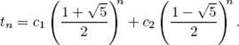
5. Substitute the constants into the general solution to obtain the particular solution:
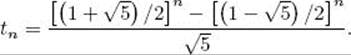
Although Example B.9 provides an explicit formula for the nth Fibonacci term, it has little practical value, because the degree of precision necessary to represent √5 increases as n increases.
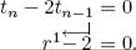
Theorem B.1 requires that all k roots of the characteristic equation be distinct. The theorem does not allow a characteristic equation of the following form:
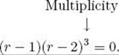
Because the term r −2 is raised to the third power, 2 is called a root of multiplicity 3 of the equation. The following theorem allows for a root to have a multiplicity. The proof of the theorem appears near the end of this appendix.
![]() Theorem B.2
Theorem B.2
Let r be a root of multiplicity m of the characteristic equation for a homogeneous linear recurrence with constant coefficients. Then
![]()
are all solutions to the recurrence. Therefore, a term for each of these solutions is included in the general solution (as given in Theorem B. 1) to the recurrence.
Example applications of this theorem follow.
Example B.10
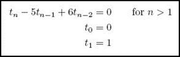
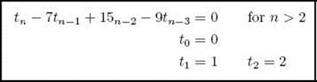
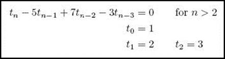
We solve the recurrence
1. Obtain the characteristic equation:
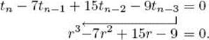
2. Solve the characteristic equation:
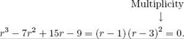
The roots are r = 1 and r = 3, and r = 3 is a root of multiplicity 2.
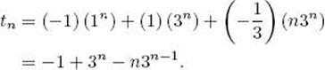
3. Apply Theorem B.2 to get the general solution to the recurrence:
![]()
We have included terms for 3n and n3n because 3 is a root of multiplicity 2.
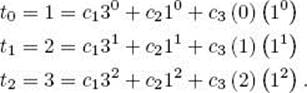
4. Determine the values of the constants by applying the general solution to the initial conditions:
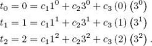
These values simplify to
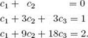
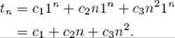
Solving this system yields c1 = −1, c2 = 1, and c3 = ![]()
5. Substitute the constants into the general solution to obtain the particular solution:
Example B.11
We solve the recurrence
1. Obtain the characteristic equation:
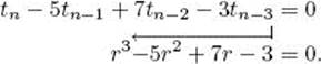
2. Solve the characteristic equation:
The roots are r = 3 and r = 1, and the root 1 has multiplicity 2.
3. Apply Theorem B.2 to obtain the general solution to the recurrence:
![]()
4. Determine the values of the constants by applying the general solution to the initial conditions:
These equations simplify to
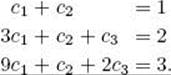
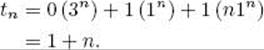
Solving this system yields c1 = 0, c2 = 1, and c3 = 1.
5. Substitute the constants into the general solution to obtain the particular solution:
• B.2.2 Nonhomogeneous Linear Recurrences
Definition
A recurrence of the form
![]()
where k and the ai terms are constants and f(n) is a function other than the zero function, is called a nonhomogeneous linear recurrence equation with constant coefficients.
By the zero function, we mean the function f(n) = 0. If we used the zero function, we would have a homogeneous linear recurrence equation. There is no known general method for solving a nonhomogeneous linear recurrence equation. We develop a method for solving the common special case
![]()
where b is a constant and p (n) is a polynomial in n.
Example B.12
The recurrence
![]()
is an example of Recurrence B.2 in which k = 1, b = 4, and p (n) = 1.
Example B.13
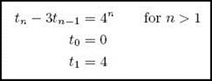
The recurrence
![]()
is an example of Recurrence B.2 in which k = 1, b = 4, and p (n) = 8n + 7.
The special case shown in Recurrence B.2 can be solved by transforming it into a homogeneous linear recurrence. The next sample illustrates how this is done.
Example B.14
We solve the recurrence
The recurrence is not homogeneous because of the term 4n on the right. We can get rid of that term as follows:
1. Replace n with n − 1 in the original recurrence so that the recurrence is expressed with 4n−1 on the right:
![]()
2. Divide the original recurrence by 4 so that the recurrence is expressed in another way with 4n−1 on the right:
![]()
3. Our original recurrence must have the same solutions as these versions of it. Therefore, it must also have the same solutions as their difference. This means we can get rid of the term 4n−1 by subtracting the recurrence obtained in Step 1 from the recurrence obtained in Step 2. The result is
![]()
We can multiply by 4 to get rid of the fractions:
![]()
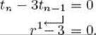
This is a homogeneous linear recurrence equation, which means that it can be solved by applying Theorem B.1. That is, we solve the characteristic equation
![]()
obtain the general solution
![]()
and use the initial conditions t0 = 0 and t1 = 4 to determine the particular solution:
![]()
In Example B.14, the general solution has the terms
![]()
The first term comes from the characteristic equation that would be obtained if the recurrence were homogeneous, whereas the second term comes from the nonhomogeneous part of the recurrence—namely, b. The polynomial p (n) in this example equals 1. When this is not the case, the manipulations necessary to transform the recurrence into a homogeneous one are more complex. However, the outcome is simply to give b a multiplicity in the characteristic equation for the resultant homogeneous linear recurrence. This result is given in the theorem that follows. The theorem is stated without proof. The proof would follow steps similar to those in Example B.14.
![]() Theorem B.3
Theorem B.3
A nonhomogeneous linear recurrence of the form
![]()
can be transformed into a homogeneous linear recurrence that has the characteristic equation
![]()
where d is the degree of p (n). Notice that the characteristic equation is composed of two parts:
1. The characteristic equation for the corresponding homogeneous recurrence
2. A term obtained from the nonhomogeneous part of the recurrence
If there is more than one term like bnp (n) on the right side, each one contributes a term to the characteristic equation.
Before applying this theorem, we recall that the degree of a polynomial p (n) is the highest power of n. For example,
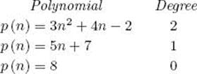
Now let’s apply Theorem B.3.
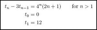
Example B.15
solve the recurrence
1. Obtain the characteristic equation for the corresponding homogeneous equation:
2. Obtain a term from the nonhomogeneous part of the recurrence:
The term from the nonhomogeneous part is
![]()
3. Apply Theorem B.3 to obtain the characteristic equation from the terms obtained in Steps 1 and 2. The characteristic equation is
![]()
After obtaining the characteristic equation, proceed exactly as in the linear homogeneous case:
4. Solve the characteristic equation:
![]()
The roots are r = 3 and r = 4, and the root r = 4 has multiplicity 2.
5. Apply Theorem B.2 to get the general solution to the recurrence:
![]()
We have three unknowns, but only two initial conditions. In this case, we must find another initial condition by computing the value of the recurrence at the next-largest value of n. In this case, that value is 2. Because
![]()
and t1 = 12,
![]()
In the exercises you are asked to (6) determine the values of the constants and (7) substitute the constants into the general solution to obtain
![]()
Example B.16
We solve the recurrence
1. Obtain the characteristic equation for the corresponding homogeneous recurrence:
2. Obtain a term from the nonhomogeneous part of the recurrence:
The term is
![]()
3. Apply Theorem B.3 to obtain the characteristic equation from the terms obtained in Steps 1 and 2. The characteristic equation is
![]()
4. Solve the characteristic equation:
![]()
The root is r = 1, and it has a multiplicity of 3.
5. Apply Theorem B.2 to get the general solution to the recurrence:
We need two more initial conditions:
![]()
In the exercises you are asked to (6) determine the values of the constants and (7) substitute the constants into the general solution to obtain
![]()
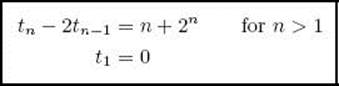
Example B.17
We solve the recurrence
1. Determine the characteristic equation for the corresponding homogeneous recurrence:
2. This is a case in which there are two terms on the right. As Theorem B.3 states, each term contributes to the characteristic equation, as follows:
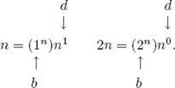
The two terms are
![]()
3. Apply Theorem B.3 to obtain the characteristic equation from all the terms:
![]()
You are asked to complete this problem in the exercises.
• B.2.3 Change of Variables (Domain Transformations)
Sometimes a recurrence that is not in the form that can be solved by applying Theorem B.3 can be solved by performing a change of variables to transform it into a new recurrence that is in that form. The technique is illustrated in the following examples. In these examples, we use T (n) for the original recurrence, because tk is used for the new recurrence. The notation T (n) means the same things as tn—namely, that a unique number is associated with each value of n.
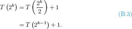
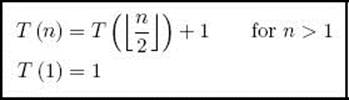
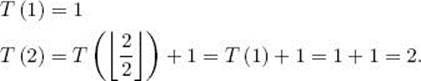
Example B.18
We solve the recurrence
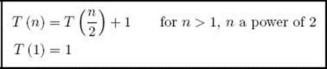
Recall that we already solved this recurrence using induction in Section B.1. We solve it again to illustrate the change of variables technique. The recurrence is not in the form that can be solved by applying Theorem B.3 because of the term n/2. We can transform it into a recurrence that is in that form as follows. First, set
![]()
Second, substitute 2k for n in the recurrence to obtain
Next, set
![]()
in Recurrence B.3 to obtain the new recurrence,
![]()
This new recurrence is in the form that can be solved by applying Theorem B.3. Therefore, applying that theorem, we can determine its general solution to be
![]()
The general solution to our original recurrence can now be obtained with the following two steps:
1. Substitute T(2k) for tk in the general solution to the new recurrence:
![]()
2. Substitute n for 2k and lg n for k in the equation obtained in Step 1:
![]()
Once we have the general solution to our original recurrence, we proceed as usual. That is, we use the initial condition T (1) = 1, determine a second initial condition, and then compute the values of the constants to obtain
![]()
Example B.19
We solve the recurrence
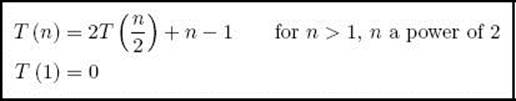
Recall that we were unable to solve this recurrence using induction in Example B.3. We solve it here with a change of variables. First, substitute 2k for n to yield
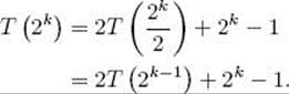
Next, set
![]()
in this equation to obtain
![]()
Apply Theorem B.3 to this new recurrence to obtain
![]()
Perform the steps that give the general solution to the original recurrence:
1. Substitute T (2k) for tk in the general solution to the new recurrence:
![]()
2. Substitute n for 2k and lg n for k in the equation obtained in Step 1:
![]()
Now proceed as usual. That is, use the initial condition T (1) = 0, determine two more initial conditions, and then compute the values of the constants. The solution is
![]()
Example B.20
We solve the recurrence
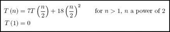
Substitute 2k for n in the recurrence to yield
![]()
Set
![]()
in Recurrence (B.4) to obtain
![]()
This recurrence does not look exactly like the kind required in Theorem B.3, but we can make it look like that as follows:
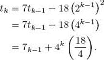
Now apply Theorem B.3 to this new recurrence to obtain
![]()
Perform the steps that give the general solution to the original recurrence:
1. Substitute T (2k) for tk in the general solution to tk:
![]()
2. Substitute n for 2k and lg n for k in the equation obtained in Step 1:
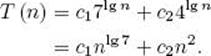
Use the initial condition T (1) = 0, determine a second initial condition, and then compute the values of the constants. The solution is
![]()
B.3 Solving Recurrences by Substitution
Sometimes a recurrence can be solved using a technique called substitution. You can try this method if you cannot obtain a solution using the methods in the last two sections. The following examples illustrate the substitution method.
Example B.21
We solve the recurrence
In a sense, substitution is the opposite of induction. That is, we start at n and work backward:
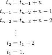
We then substitute each equality into the previous one, as follows:
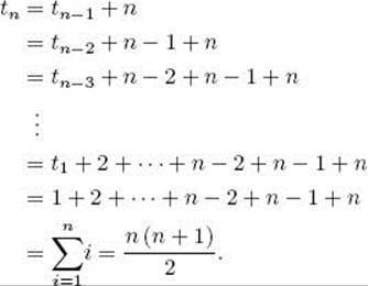
The last equality is the result in Example A.1 in Appendix A.
The recurrence in Example B.21 could be solved using the characteristic equation. The recurrence in the following example cannot.
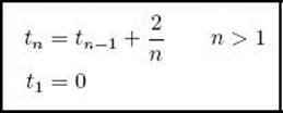
Example B.22
We solve the recurrence
First, work backward from n:
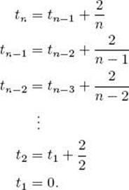
Then substitute each equation into the previous one:
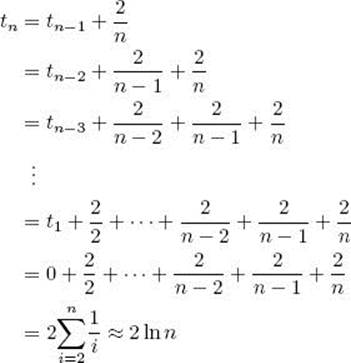
for n not small. The approximate equality is obtained from Example A.9 in Appendix A.
B.4 Extending Results for n, a Power of a Positive Constant b, to n in General
It is assumed in the material that follows that you are familiar with the material in Chapter 1.
In the case of some recursive algorithms, we can readily determine the exact time complexity only when n is a power of some base b, where b is a positive constant. Often the base b is 2. This is true in particular for many divide-and-conquer algorithms (see Chapter 2). Intuitively, it seems that a result that holds for n a power of b should approximately hold for n in general. For example, if for some algorithm we establish that
![]()
for n a power of 2, it seems that for n in general we should be able to conclude that
![]()
It turns out that usually we can draw such a conclusion. Next we discuss situations in which this is the case. First we need some definitions. These definitions apply to arbitrary functions whose domains and ranges are any subsets of the real numbers, but we state them for complexity functions (that is, functions that map the positive integers to the positive reals) because these are the functions that interest us here.
Definition
A complexity function f(n) is called strictly increasing if f(n) always gets larger as n gets larger. That is, if n1 > n2, then
![]()
The function shown in Figure B.1(a) is strictly increasing. (For clarity, the domains of the functions in Figure B.1 are all the nonnegative reals.) Many of the functions we encounter in algorithm analysis are strictly increasing for nonnegative values of n. For example, lg n, n, n lg n, n2, and 2n are all strictly increasing as long as n is nonnegative.
Definition
A complexity function f(n) is called nondecreasing if f(n) never gets smaller as n gets larger. That is, if n1 > n2, then
![]()
Figure B.1 Four functions.
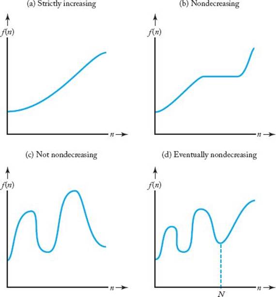
Any strictly increasing function is nondecreasing, but a function that can level out is nondecreasing without being strictly increasing. The function shown in Figure B.1(b) is an example of such a function. The function in Figure B.1(c) is not nondecreasing.
The time (or memory) complexities of most algorithms are ordinarily nondecreasing because the time it takes to process an input usually does not decrease as the input size becomes larger. Looking at Figure B.1, it seems that we should be able to extend an analysis for n a power of b to n in general as long as the function is nondecreasing. For example, suppose we have determined the values of f(n) for n a power of 2. In the case of the function in Figure B.1(c), anything can happen between, say, 23 = 8 and 24 = 16. Therefore, nothing can be concluded about the behavior of the function between 8 and 16 from the values at 8 and 16. However, in the case of a nondecreasing function f(n), if 8 ≤ n ≤ 16 then
![]()
So it seems that we should be able to determine the order of f(n) from the values of f(n) for n a power of 2. What seems to be true intuitively can indeed be proven for a large class of functions. Before giving a theorem stating this, we recall that order has to do only with long-range behavior. Because initial values of a function are unimportant, the theorem requires only that the function be eventually nondecreasing. We have the following definition:
Definition
A complexity function f(n) is called eventually nondecreasing if for all n past some point the function never gets smaller as n gets larger. That is, there exists an N such that if n1 > n2 > N, then
![]()
Any nondecreasing function is eventually nondecreasing. The function shown in Figure 3.1(d) is an example of an eventually nondecreasing function that is not nondecreasing. We need the following definition before we give the theorem for extending the results for n a power of b:
Definition
A complexity function f(n) is called smooth if f(n) is eventually nondecreasing and if
![]()
Example B.23
The functions lg n, n, n lg n, and nk, where k ≥ 0, are all smooth. We show this for lg n. In the exercises you are asked to show it for the other functions. We have already noted that lg n is eventually nondecreasing. As to the second condition, we have
![]()
Example B.24
The function 2n is not smooth, because the Properties of Order in Section 1.4.2 in Chapter 1 imply that
![]()
Therefore,
![]()
We now state the theorem that enables us to generalize results obtained for n a power of b. The proof appears near the end of this appendix.
![]() Theorem B.4
Theorem B.4
Let b ≥ 2 be an integer, let f(n) be a smooth complexity function, and let T (n) be an eventually nondecreasing complexity function. If
![]()
then
![]()
Furthermore, the same implication holds if Θ is replaced by “big O,” Ω, or “small o.”
By “T (n) ![]() Θ(f(n)) for n a power of b,” we mean that the usual conditions for Θ are known to hold when n is restricted to being a power of b. Notice in Theorem B.4 the additional requirement that f(n) be smooth.
Θ(f(n)) for n a power of b,” we mean that the usual conditions for Θ are known to hold when n is restricted to being a power of b. Notice in Theorem B.4 the additional requirement that f(n) be smooth.
Next we apply Theorem B.4
![]() Example B.25
Example B.25
Suppose for some complexity function we establish that
When n is a power of 2, we have the recurrence in Example B.18. Therefore, by that example,
![]()
Because lg n is smooth, we need only show that T (n) is eventually nonde-creasing in order to apply Theorem B.4 to conclude that
![]()
One might be tempted to conclude that T (n) is eventually nondecreasing from the fact that lg n + 1 is eventually nondecreasing. However, we cannot do this because we know only that T (n) = lg n + 1 when n is a power of 2. Given only this fact, T (n) could exhibit any possible behavior in between powers of 2.
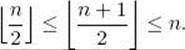
We show that T (n) is eventually nondecreasing by using induction to establish for n ≥ 2 that if 1 ≤ k < n, then
![]()
Induction base: For n = 2,
Therefore,
![]()
Induction hypothesis: One way to make the induction hypothesis is to assume that the statement is true for all m ≤ n. Then, as usual, we show that it is true for n + 1. This is the way we need it to be stated here. Let n be an arbitrary integer greater than or equal to 2. Assume for all m ≤ n that if k <m, then
![]()
Induction step: Because in the induction hypothesis we assumed for k < n that
![]()
we need only show that
![]()
To that end, it is not hard to see that if n ≥ 1, then
Therefore, by the induction hypothesis,
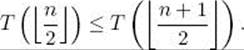
Using the recurrence, we have

and we are done.
Finally, we develop a general method for determining the order of some common recurrences.
![]() Theorem B.5
Theorem B.5
Suppose a complexity function T (n) is eventually nondecreasing and satisfies
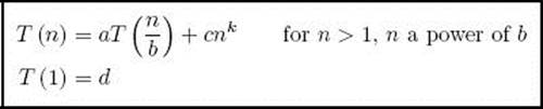
where b ≥ 2 and k ≥ 0 are constant integers, and a, c, and d are constants such that a > 0, c > 0, and d ≥ 0. Then
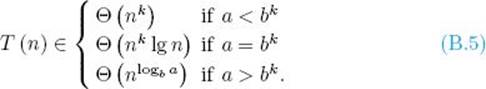
Furthermore, if, in the statement of the recurrence,
![]()
is replaced by
![]()
then Result B.5 holds with “big O” or Ω, respectively, replacing Θ.
We can prove this theorem by solving the general recurrence using the characteristic equation and then applying Theorem B.4. Example applications of Theorem B.5 follow.
Example B.26
Suppose that T (n) is eventually nondecreasing and satisfies
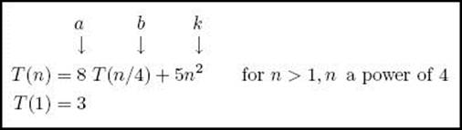
By Theorem B.5, because 8 < 42,
![]()
Example B.27
Suppose that T (n) is eventually nondecreasing and satisfies
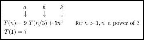
By Theorem B.5, because 9 > 31,
![]()
Theorem B.5 was stated in order to introduce an important theorem as simply as possible. It is actually the special case, in which the constant s equals 1, of the following theorem.
![]() Theorem B.6
Theorem B.6
Suppose that a complexity function T (n) is eventually nondecreasing and satisfies
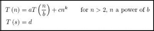
where s is a constant that is a power of b, b ≥ 2 and k ≥ 0 are constant integers, and a, c, and d are constants such that a > 0, c > 0, and d ≥ 0. Then the results in Theorem B.5 still hold.
Example B.28
Suppose that T (n) is eventually nondecreasing and satisfies
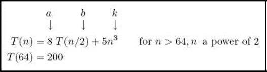
By Theorem B.6, because 8 = 23,
![]()
This concludes our discussion of techniques for solving recurrences. Another technique is to use “generating functions” to solve recurrences. This technique is discussed in Sahni (1988). Bentley, Haken, and Sax (1980) provide a general method for solving recurrences arising from the analysis of divide-and-conquer algorithms (see Chapter 2).
B.5 Proofs of Theorems
The following lemma is needed to prove Theorem B.1.
![]() Lemma B.1
Lemma B.1
Suppose we have the homogeneous linear recurrence
![]()
If r1 is a root of the characteristic equation
![]()
then
![]()
is a solution to the recurrence.
Proof: If, for i = n − k,..., n, we substitute ri1 for ti in the recurrence, we obtain
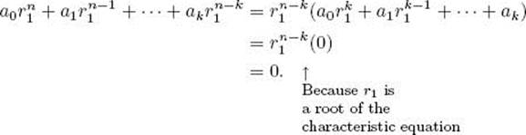
Therefore, r1n is a solution to the recurrence.
Proof of Theorem B.1 It is not hard to see that, for a linear homogeneous recurrence, a constant times any solution and the sum of any two solutions are each solutions to the recurrence. We can therefore apply Lemma B.1 to conclude that, if
![]()
are the k distinct roots of the characteristic equation, then
![]()
where the ci terms are arbitrary constants, is a solution to the recurrence. Although we do not show it here, one can prove that these are the only solutions.
![]() Proof of Theorem B.2 We prove the case where the multiplicity m equals 2. The case of a larger m is a straightforward generalization. Let r1 be a root of multiplicity 2. Set
Proof of Theorem B.2 We prove the case where the multiplicity m equals 2. The case of a larger m is a straightforward generalization. Let r1 be a root of multiplicity 2. Set
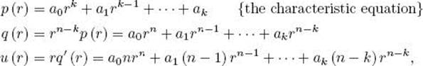
where q′ (r) means the first derivative. If we substitute ![]() for ti in the recurrence, we obtain u (r1). Therefore, if we can show that u (r1) = 0, we can conclude that
for ti in the recurrence, we obtain u (r1). Therefore, if we can show that u (r1) = 0, we can conclude that ![]() is a solution to the recurrence, and we are done. To this end, we have
is a solution to the recurrence, and we are done. To this end, we have
Therefore, to show that u (r1) = 0, we need only show that p (r1) and p′ (r1) both equal 0. We show this as follows. Because r1 is a solution of multiplicity 2 of the characteristic equation p (r), there exists a v (r) such that
![]()
Therefore,
![]()
and p (r1) and p′ (r1) both equal 0. This completes the proof.
![]() Proof of Theorem B.4 We obtain the proof for “big O.” Proofs for Ω and Θ can be established in a similar manner. Because T (n)
Proof of Theorem B.4 We obtain the proof for “big O.” Proofs for Ω and Θ can be established in a similar manner. Because T (n) ![]() O (f(n)) for all n such that n is a power of b, there exist a positive c1 and a nonnegative integer N1 such that, for n > N1 and n a power of b,
O (f(n)) for all n such that n is a power of b, there exist a positive c1 and a nonnegative integer N1 such that, for n > N1 and n a power of b,
![]()
For any positive integer n, there exists a unique k such that
![]()
It is possible to show, in the case of a smooth function, that, if b ≥ 2, then
![]()
That is, if this condition holds for 2, it holds for any b > 2. Therefore, there exist a positive constant c2 and a nonnegative integer N2 such that, for n > N2,
![]()
Therefore, if bk≥ N2,
![]()
Because T (n) and f(n) are both eventually nondecreasing, there exists an N3, such that, for m > n > N3,
![]()
Let r be so large that
![]()
If n > br and k is the value corresponding to n in Inequality B.7, then
![]()
Therefore, by Inequalities B.6, B.7, B.8, and B.9, for n > br,
![]()
which means that
![]()
EXERCISES
Section B.1
1. Use induction to verify the candidate solution to each of the following recurrence equations.
(a) tn = 4tn−1 for n > 1
t1 = 3
The candidate solution is tn = 3 (4n−1).
(b) tn = tn−1 + 5 for n > 1
t1 = 2
The candidate solution is tn = 5n − 3.
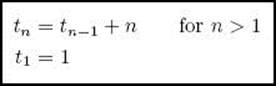
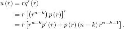
(c) tn = tn−1 + n for n > 1
t1 = 1
The candidate solution is ![]()
(d) tn = tn−1 + n2 for n > 1
t1 = 1
The candidate solution is ![]()
(e) 
The candidate solution is
(f) tn = 3tn−1 + 2n for n > 1
t1 = 1
The candidate solution is
(g) 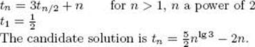
The candidate solution is tn = 5
(h) tn = ntn−1 for n > 0
t0 = 1
The candidate solution is tn = n!.
2. Write a recurrence equation for the nth term of the sequence 2, 6, 18, 54,..., and use induction to verify the candidate solution sn = 2 (3n−1)
3. The number of moves (mn for n rings) needed in the Towers of Hanoi problem (see Exercise 17 in Chapter 2) is given by the following recurrence equation
![]()
Use induction to show that the solution to this recurrence equation is mn = 2n − 1.
4. The following algorithm returns the position of the largest element in the array S. Write a recurrence equation for the number of comparisons tn needed to find the largest element. Use induction to show that the equation has the solution tn = n − 1.
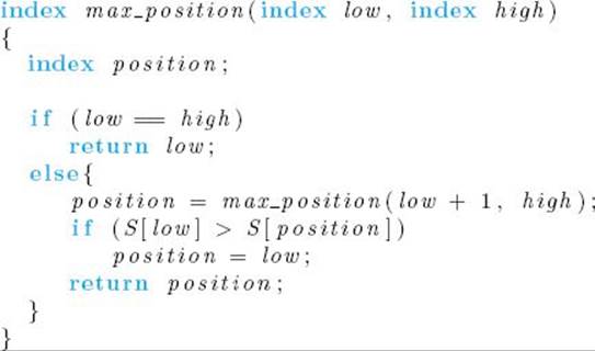
The top-level call is
max position (1, n).
5. The ancient Greeks were very interested in sequences resulting from geometric shapes such as the following triangular numbers:
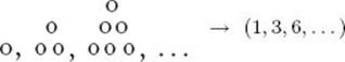
Write a recurrence equation for the nth term in this sequence, guess a solution, and use induction to verify your solution.
6. Into how many regions do n lines divide a plane so that every pair of lines intersect, but no more than two lines intersect at a common point? Write a recurrence equation for the number of regions for n lines, guess a solution for your equation, and use induction to verify your solution.
7. Show that 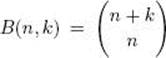 is the solution to the following recurrence equation:
8. Write and implement an algorithm that computes the value of the following recurrence, and run it using different problem instances. Use the results to guess a solution for this recurrence, and use induction to verify your solution.
![]()
Section B.2
9. Indicate which recurrence equations in the problems for Section B.1 fall into each of the following categories.
(a) Linear equations
(b) Homogeneous equations
(c) Equations with constant coefficients
10. Find the characteristic equations for all of the recurrence equations in Section B.1 that are linear with constant coefficients.
11. Show that if f(n) and g (n) are both solutions to a linear homogeneous recurrence equation with constant coefficients, then so is c × f(n) + d × g(n), where c and d are constants.
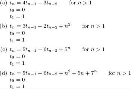
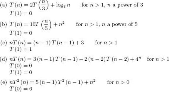
12. Solve the following recurrence equations using the characteristic equation.
13. Complete the solution to the recurrence equation given in Example B.15.
14. Complete the solution to the recurrence equation given in Example B.16.
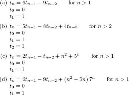
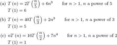
15. Solve the following recurrence equations using the characteristic equation.
16. Complete the solution to the recurrence equation given in Example B. 17.
17. Show that the recurrence equation
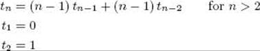
can be written as
![]()
18. Solve the recurrence equation in Exercise 17. The solution gives the number of derangements (nothing is in its right place) of n objects.
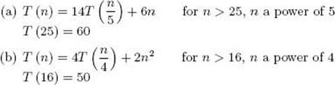
19. Solve the following recurrence equations using the characteristic equation.
Section B.3
20. Solve the recurrence equations in Exercise 1 using the substitution method.
Section B.4
21. Show that
(a) f(n) = n3 is a strictly increasing function.
(b) g (n) = 2n3 − 6n2 is an eventually nondecreasing function.
22. What can we say about a function f(n) that is both nondecreasing and nonincreasing for all values of n?
23. Show that the following functions are smooth.
(a) f(n) = n lg n
(b) g (n) = nk, for all k ≥ 0.
24. Assuming in each case that T (n) is eventually nondecreasing, use Theorem B.5 to determine the order of the following recurrence equations.
25. Assuming in each case that T (n) is eventually nondecreasing, use Theorem B.6 to determine the order of the following recurrence equations:
26. We know that the recurrence
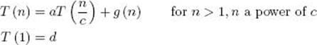
has solution
![]()
in the case a > c, provided that g (n) ![]() Θ(n). Prove that the recurrence has the same solution if we assume that
Θ(n). Prove that the recurrence has the same solution if we assume that
![]()
All materials on the site are licensed Creative Commons Attribution-Sharealike 3.0 Unported CC BY-SA 3.0 & GNU Free Documentation License (GFDL)
If you are the copyright holder of any material contained on our site and intend to remove it, please contact our site administrator for approval.
© 2016-2026 All site design rights belong to S.Y.A.