Foundations of Algorithms (2015)

Chapter 2 Divide-and-Conquer

Our first approach to designing algorithms, divide-and-conquer, is patterned after the brilliant strategy employed by the French emperor Napoleon in the Battle of Austerlitz on December 2, 1805. A combined army of Austrians and Russians outnumbered Napoleon’s army by about 15,000 soldiers. The Austro-Russian army launched a massive attack against the French right flank. Anticipating their attack, Napoleon drove against their center and split their forces in two. Because the two smaller armies were individually no match for Napoleon, they each suffered heavy losses and were compelled to retreat. By dividing the large army into two smaller armies and individually conquering these two smaller armies, Napoleon was able to conquer the large army.

The divide-and-conquer approach employs this same strategy on an instance of a problem. That is, it divides an instance of a problem into two or more smaller instances. The smaller instances are usually instances of the original problem. If solutions to the smaller instances can be obtained readily, the solution to the original instance can be obtained by combining these solutions. If the smaller instances are still too large to be solved readily, they can be divided into still smaller instances. This process of dividing the instances continues until they are so small that a solution is readily obtainable.

The divide-and-conquer approach is a top-down approach. That is, the solution to a top-level instance of a problem is obtained by going down and obtaining solutions to smaller instances. The reader may recognize this as the method used by recursive routines. Recall that when writing recursion, one thinks at the problem-solving level and lets the system handle the details of obtaining the solution (by means of stack manipulations). When developing a divide-and-conquer algorithm, we usually think at this level and write it as a recursive routine. After this, we can sometimes create a more efficient iterative version of the algorithm.

We now introduce the divide-and-conquer approach with examples, starting with Binary Search.

2.1 Binary Search

We showed an iterative version of Binary Search (Algorithm 1.5) in Section 1.2. Here we present a recursive version because recursion illustrates the top-down approach used by divide-and-conquer. Stated in divide-and-conquer terminology, Binary Search locates a key x in a sorted (nondecreasing order) array by first comparing x with the middle item of the array. If they are equal, the algorithm is done. If not, the array is divided into two subarrays, one containing all the items to the left of the middle item and the other containing all the items to the right. If x is smaller than the middle item, this procedure is then applied to the left subarray. Otherwise, it is applied to the right subarray. That is, x is compared with the middle item of the appropriate subarray. If they are equal, the algorithm is done. If not, the subarray is divided in two. This procedure is repeated until x is found or it is determined that x is not in the array.

The steps of Binary Search can be summarized as follows.

If x equals the middle item, quit. Otherwise:

1. Divide the array into two subarrays about half as large. If x is smaller than the middle item, choose the left subarray. If x is larger than the middle item, choose the right subarray.

2. Conquer (solve) the subarray by determining whether x is in that subarray. Unless the subarray is sufficiently small, use recursion to do this.

3. Obtain the solution to the array from the solution to the subarray.

Binary Search is the simplest kind of divide-and-conquer algorithm because the instance is broken down into only one smaller instance, so there is no combination of outputs. The solution to the original instance is simply the solution to the smaller instance. The following example illustrates Binary Search.

Example 2.1

Suppose x = 18 and we have the following array:

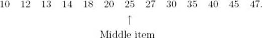
1. Divide the array: Because x < 25, we need to search

2. Conquer the subarray by determining whether x is in the subarray. This is accomplished by recursively dividing the subarray. The solution is:

Yes, x is in the subarray.

3. Obtain the solution to the array from the solution to the subarray:

Yes, x is in the array.

In Step 2 we simply assumed that the solution to the subarray was available. We did not discuss all the details involved in obtaining the solution because we wanted to show the solution at a problem-solving level. When developing a recursive algorithm for a problem, we need to

• Develop a way to obtain the solution to an instance from the solution to one or more smaller instances.

• Determine the terminal condition(s) that the smaller instance(s) is (are) approaching.

• Determine the solution in the case of the terminal condition(s).

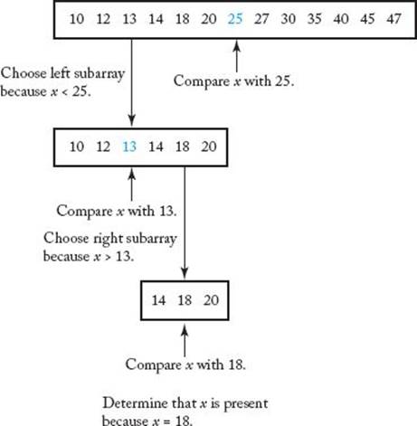
We need not be concerned with the details of how the solution is obtained (in the case of a computer, by means of stack manipulations). Indeed, worrying about these details can sometimes hinder one’s development of a complex recursive algorithm. For the sake of concreteness, Figure 2.1shows the steps done by a human when searching with Binary Search.

A recursive version of Binary Search now follows.

Algorithm 2.1

Binary Search (Recursive)

Problem: Determine whether x is in the sorted array S of size n.

Inputs: positive integer n, sorted (nondecreasing order) array of keys S indexed from 1 to n, a key x.

Outputs: location, the location of x in S (0 if x is not in S).

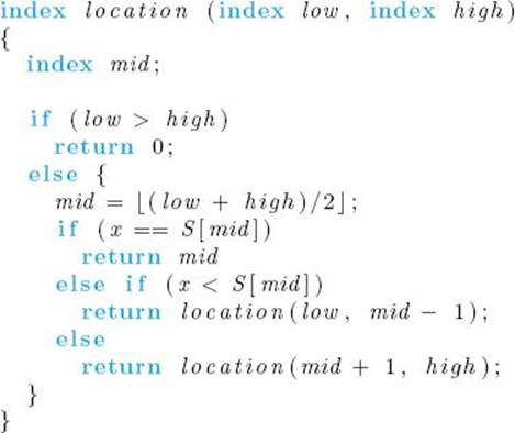
Notice that n, S, and x are not parameters to function location. Because they remain unchanged in each recursive call, there is no need to make them parameters. In this text only the variables, whose values can change in the recursive calls, are made parameters to recursive routines. There are two reasons for doing this. First, it makes the expression of recursive routines less cluttered. Second, in an actual implementation of a recursive routine, a new copy of any variable passed to the routine is made in each recursive call. If a variable’s value does not change, the copy is unnecessary. This waste could be costly if the variable is an array. One way to circumvent this problem would be to pass the variable by address. Indeed, if the implementation language is C++, an array is automatically passed by address, and using the reserved word const guarantees the array cannot be modified. However, including all of this in our pseudocode expression of recursive algorithms again serves to clutter them and possibly diminish their clarity.

Figure 2.1 The steps done by a human when searching with Binary Search. (Note: x = 18.)

Each of the recursive algorithms could be implemented in a number of ways, depending on the language used for the implementation. For example, one possible way to implement them in C++ would be pass all the parameters to the recursive routine; another would be to use classes; and yet another would be to globally define the parameters that do not change in the recursive calls. We will illustrate how to implement the last one since this is the alternative consistent with our expression of the algorithms. If we did define S and x globally and n was the number of items in S, our top-level call to function location in Algorithm 2.1 would be as follows:

locationout = location (1 , n) ;

Because the recursive version of Binary Search employs tail-recursion (that is, no operations are done after the recursive call), it is straightforward to produce an iterative version, as was done in Section 1.2. As previously discussed, we have written a recursive version because recursion clearly illustrates the divide-and-conquer process of dividing an instance into smaller instances. However, it is advantageous in languages such as C++ to replace tail-recursion by iteration. Most importantly, a substantial amount of memory can be saved by eliminating the stack developed in the recursive calls. Recall that when a routine calls another routine, it is necessary to save the first routine’s pending results by pushing them onto the stack of activation records. If the second routine calls another routine, the second routine’s pending results must also be pushed onto the stack, and so on. When control is returned to a calling routine, its activation record is popped from the stack and the computation of the pending results is completed. In the case of a recursive routine, the number of activation records pushed onto the stack is determined by the depth reached in the recursive calls. For Binary Search, the stack reaches a depth that in the worst case is about lg n + 1.

Another reason for replacing tail-recursion by iteration is that the iterative algorithm will execute faster (but only by a constant multiplicative factor) than the recursive version because no stack needs to be maintained. Because most modern LISP dialects compile tail-recursion to iterative code, there is no reason to replace tail-recursion by iteration in these dialects.

Binary Search does not have an every-case time complexity. We will do a worst-case analysis. We already did this informally in Section 1.2. Here we do the analysis more rigorously. Although the analysis refers to Algorithm 2.1, it pertains to Algorithm 1.5 as well. If you are not familiar with techniques for solving recurrence equations, you should study Appendix B before proceeding.

Analysis of Algorithm 2.1

Worst-Case Time Complexity (Binary Search, Recursive)

In an algorithm that searches an array, the most costly operation is usually the comparison of the search item with an array item. Thus, we have the following:

Basic operation: the comparison of x with S [mid].

Input size: n, the number of items in the array.

We first analyze the case in which n is a power of 2. There are two comparisons of x with S [mid] in any call to function location in which x does not equal S [mid]. However, as discussed in our informal analysis of Binary Search in Section 1.2, we can assume that there is only one comparison, because this would be the case in an efficient assembler language implementation. Recall from Section 1.3 that we ordinarily assume that the basic operation is implemented as efficiently as possible.

As discussed in Section 1.2, one way the worst case can occur is when x is larger than all array items. If n is a power of 2 and x is larger than all the array items, each recursive call reduces the instance to one exactly half as big. For example, if n = 16, then mid = (1 + 16) /2 = 8. Because x is larger than all the array items, the top eight items are the input to the first recursive call. Similarly, the top four items are the input to the second recursive call, and so on. We have the following recurrence:

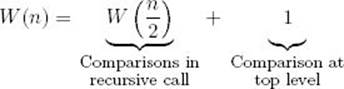
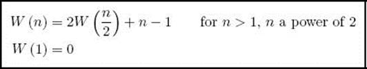
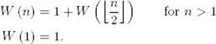
If n = 1 and x is larger than the single array item, there is a comparison of x with that item followed by a recursive call with low > high. At this point the terminal condition is true, which means that there are no more comparisons. Therefore, W (1) is 1. We have established the recurrence

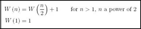
This recurrence is solved in Example B.1 in Appendix B. The solution is

If n is not restricted to being a power of 2, then

where y means the greatest integer less than or equal to y. We show how to establish this result in the exercises.

2.2 Mergesort

A process related to sorting is merging. By two-way merging we mean combining two sorted arrays into one sorted array. By repeatedly applying the merging procedure, we can sort an array. For example, to sort an array of 16 items, we can divide it into two subarrays, each of size 8, sort the two subarrays, and then merge them to produce the sorted array. In the same way, each subarray of size 8 can be divided into two subarrays of size 4, and these subarrays can be sorted and merged. Eventually, the size of the subarrays will become 1, and an array of size 1 is trivially sorted. This procedure is called “Mergesort.” Given an array with n items (for simplicity, let n be a power of 2), Mergesort involves the following steps:

1. Divide the array into two subarrays each with n/2 items.

2. Conquer (solve) each subarray by sorting it. Unless the array is sufficiently small, use recursion to do this.

3. Combine the solutions to the subarrays by merging them into a single sorted array.

The following example illustrates these steps.

Example 2.2

Suppose the array contains these numbers in sequence:

1. Divide the array:

2. Sort each subarray:

3. Merge the subarrays:

Figure 2.2 The steps done by a human when sorting with Mergesort.

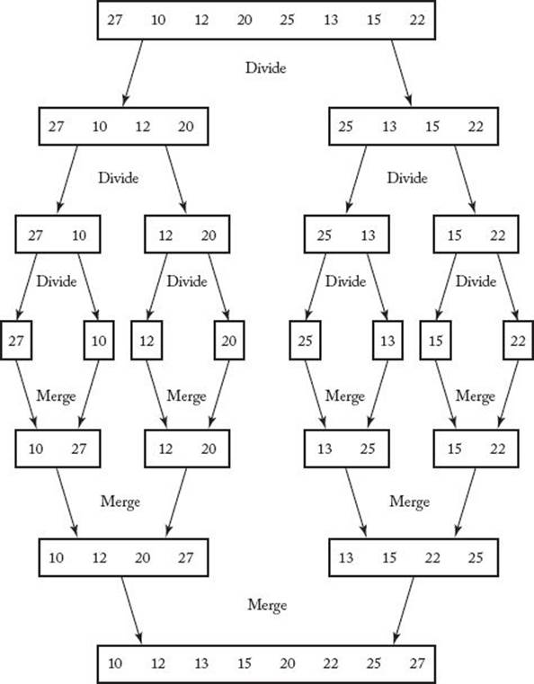
In Step 2 we think at the problem-solving level and assume that the solutions to the subarrays are available. To make matters more concrete, Figure 2.2 illustrates the steps done by a human when sorting with Mergesort. The terminal condition occurs when an array of size 1 is reached; at that time, the merging begins.

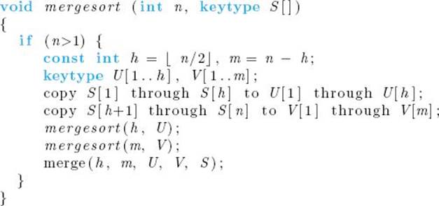
Algorithm 2.2

Mergesort

Problem: Sort n keys in nondecreasing sequence.

Inputs: positive integer n, array of keys S indexed from 1 to n.

Outputs: the array S containing the keys in nondecreasing order.

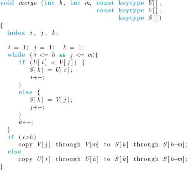
Before we can analyze Mergesort, we must write and analyze an algorithm that merges two sorted arrays.

Algorithm 2.3

Merge

Problem: Merge two sorted arrays into one sorted array.

Inputs: positive integers h and m, array of sorted keys U indexed from 1 to h, array of sorted keys V indexed from 1 to m.

Outputs: an array S indexed from 1 to h + m containing the keys in U and V in a single sorted array.

• Table 2.1 An example of merging two arrays U and V into one array S^∗

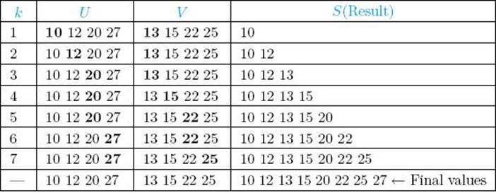
*Items compared are in boldface.

Table 2.1 illustrates how procedure merge works when merging two arrays of size 4.

Analysis of Algorithm 2.3

Worse-Case Time Complexity (Merge)

As mentioned in Section 1.3, in the case of algorithms that sort by comparing keys, the comparison instruction and the assignment instruction can each be considered the basic operation. Here we will consider the comparison instruction. When we discuss Mergesort further in Chapter 7, we will consider the number of assignments. In this algorithm, the number of comparisons depends on both h and m. We therefore have the following:

Basic operation: the comparison of U [i] with V [j].

Input size: h and m, the number of items in each of the two input arrays.

The worst case occurs when the loop is exited, because one of the indices— say, i—has reached its exit point h + 1 whereas the other index j has reached m, 1 less than its exit point. For example, this can occur when the first m − 1 items in V are placed first in S, followed by all h items in U, at which time the loop is exited because i equals h + 1. Therefore,

We can now analyze Mergesort.

Analysis of Algorithm 2.2

Worst-Case Time Complexity (Mergesort)

The basic operation is the comparison that takes place in merge. Because the number of comparisons increases with h and m, and h and m increase with n, we have the following:

Basic operation: the comparison that takes place in merge.

Input size: n, the number of items in the array S.

The total number of comparisons is the sum of the number of comparisons in the recursive call to mergesort with U as the input, the number of comparisons in the recursive call to mergesort with V as the input, and the number of comparisons in the top-level call to merge. Therefore,

We first analyze the case where n is a power of 2. In this case,

Our expression for W(n) becomes

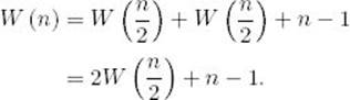
When the input size is 1, the terminal condition is met and no merging is done. Therefore, W (1) is 0. We have established the recurrence

This recurrence is solved in Example B.19 in Appendix B. The solution is

For n not a power of 2, we will establish in the exercises that

where y and y are the smallest integer ≥ y and the largest integer ≤ y, respectively. It is hard to analyze this case exactly because of the floors ( ) and ceilings ( ). However, using an induction argument like the one in Example B.25 in Appendix B, it can be shown that W(n) is nondecreasing. Therefore, Theorem B.4 in that appendix implies that

An in-place sort is a sorting algorithm that does not use any extra space beyond that needed to store the input. Algorithm 2.2 is not an in-place sort because it uses the arrays U and V besides the input array S. If U and V are variable parameters (passed by address) in merge, a second copy of these arrays will not be created when merge is called. However, new arrays U and V will still be created each time mergesort is called. At the top level, the sum of the numbers of items in these two arrays is n. In the top-level recursive call, the sum of the numbers of items in the two arrays is aboutn/2; in the recursive call at the next level, the sum of the numbers of items in the two arrays is about n/4; and, in general, the sum of the numbers of items in the two arrays at each recursion level is about one-half of the sum at the previous level. Therefore, the total number of extra array items created is about n (1 + 1/2 + 1/4 + · · ·) = 2n.

Algorithm 2.2 clearly illustrates the process of dividing an instance of a problem into smaller instances because two new arrays (smaller instances) are actually created from the input array (original instance). Therefore, this was a good way to introduce Mergesort and illustrate the divide-and-conquer approach. However, it is possible to reduce the amount of extra space to only one array containing n items. This is accomplished by doing much of the manipulation on the input array S. The following method for doing this is similar to the method used in Algorithm 2.1 (Binary Search, Recursive).

Algorithm 2.4

Mergesort 2

Problem: Sort n keys in nondecreasing sequence.

Inputs: positive integer n, array of keys S indexed from 1 to n.

Outputs: the array S containing the keys in nondecreasing order.

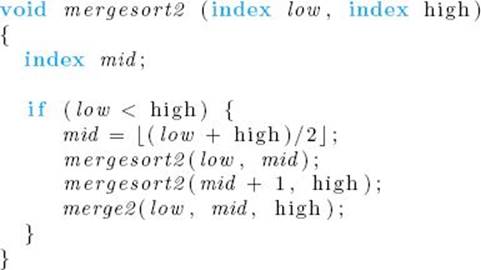
Following our convention of making only variables, whose values can change in recursive calls, parameters to recursive routines, n and S are not parameters to procedure mergesort2. If the algorithm were implemented by defining S globally and n was the number of items in S, the top-level call to mergesort2 would be as follows:

mergesort2 (1 , n) ;

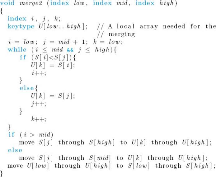
The merging procedure that works with mergesort2 follows.

Algorithm 2.5

Merge 2

Problem: Merge the two sorted subarrays of S created in Mergesort 2.

Inputs: indices low, mid, and high, and the subarray of S indexed from low to high. The keys in array slots from low to mid are already sorted in nondecreasing order, as are the keys in array slots from mid + 1 to high.

Outputs: the subarray of S indexed from low to high containing the keys in nondecreasing order.

2.3 The Divide-and-Conquer Approach

Having studied two divide-and-conquer algorithms in detail, you should now better understand the following general description of this approach.

The divide-and-conquer design strategy involves the following steps:

1. Divide an instance of a problem into one or more smaller instances.

2. Conquer (solve) each of the smaller instances. Unless a smaller instance is sufficiently small, use recursion to do this.

3. If necessary, combine the solutions to the smaller instances to obtain the solution to the original instance.

The reason we say “if necessary” in Step 3 is that in algorithms such as Binary Search Recursive (Algorithm 2.1) the instance is reduced to just one smaller instance, so there is no need to combine solutions.

More examples of the divide-and-conquer approach follow. In these examples we will not explicitly mention the steps previously outlined. It should be clear that we are following them.

2.4 Quicksort (Partition Exchange Sort)

Next we look at a sorting algorithm, called “Quicksort,” that was developed by Hoare (1962). Quicksort is similar to Mergesort in that the sort is accomplished by dividing the array into two partitions and then sorting each partition recursively. In Quicksort, however, the array is partitioned by placing all items smaller than some pivot item before that item and all items larger than the pivot item after it. The pivot item can be any item, and for convenience we will simply make it the first one. The following example illustrates how Quicksort works.

Example 2.3

Suppose the array contains these numbers in sequence:

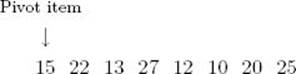
1. Partition the array so that all items smaller than the pivot item are to the left of it and all items larger are to the right:

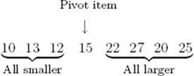
2. Sort the subarrays:

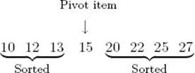
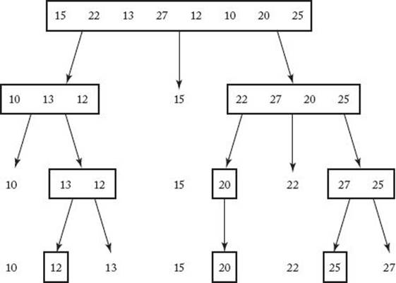
After the partitioning, the order of the items in the subarrays is unspecified and is a result of how the partitioning is implemented. We have ordered them according to how the partitioning routine, which will be presented shortly, would place them. The important thing is that all items smaller than the pivot item are to the left of it, and all items larger are to the right of it. Quicksort is then called recursively to sort each of the two subarrays. They are partitioned, and this procedure is continued until an array with one item is reached. Such an array is trivially sorted. Example 2.3 shows the solution at the problem-solving level. Figure 2.3 illustrates the steps done by a human when sorting with Quicksort. The algorithm follows.

Algorithm 2.6

Quicksort

Problem: Sort n keys in nondecreasing order.

Inputs: positive integer n, array of keys S indexed from 1 to n.

Outputs: the array S containing the keys in nondecreasing order.

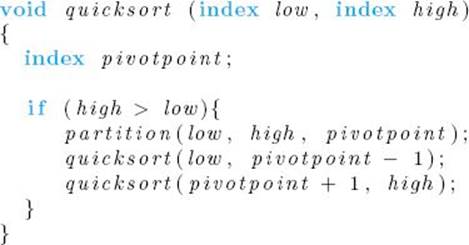
Following our usual convention, n and S are not parameters to procedure quicksort. If the algorithm were implemented by defining S globally and n was the number of items in S, the top-level call to quicksort would be as follows:

quicksort (1 , n) ;

Figure 2.3 The steps done by a human when sorting with Quicksort. The subarrays are enclosed in rectangles whereas the pivot points are free.

The partitioning of the array is done by procedure partition. Next we show an algorithm for this procedure.

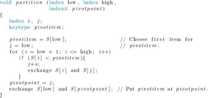
Algorithm 2.7

Partition

Problem: Partition the array S for Quicksort.

Inputs: two indices, low and high, and the subarray of S indexed from low to high.

Outputs: pivotpoint, the pivot point for the subarray indexed from low to high.

• Table 2.2 An example of procedure partition^∗

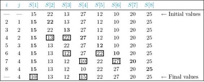
^∗ Items compared are in boldface. Items just exchanged appear in squares.

Procedure partition works by checking each item in the array in sequence. Whenever an item is found to be less than the pivot item, it is moved to the left side of the array. Table 2.2 shows how partition would proceed on the array in Example 2.3.

Next we analyze Partition and Quicksort.

Analysis of Algorithm 2.7

Every-Case Time Complexity (Partition)

Basic operation: the comparison of S [i] with pivotitem.

Input size: n = high − low + 1, the number of items in the subarray.

Because every item except the first is compared,

We are using n here to represent the size of the subarray, not the size of the array S. It represents the size of S only when partition is called at the top level.

Quicksort does not have an every-case complexity. We will do worst-case and average-case analyses.

Analysis of Algorithm 2.6

Worst-Case Time Complexity (Quicksort)

Basic operation: the comparison of S [i] with pivotitem in partition.

Input size: n, the number of items in the array S.

Oddly enough, it turns out that the worst case occurs if the array is already sorted in nondecreasing order. The reason for this should become clear. If the array is already sorted in nondecreasing order, no items are less than the first item in the array, which is the pivot item. Therefore, when partitionis called at the top level, no items are placed to the left of the pivot item, and the value of pivotpoint assigned by partition is 1. Similarly, in each recursive call, pivotpoint receives the value of low. Therefore, the array is repeatedly partitioned into an empty subarray on the left and a subarray with one less item on the right. For the class of instances that are already sorted in nondecreasing order, we have

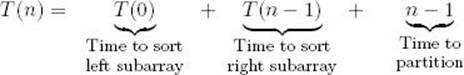
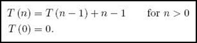
We are using the notation T(n) because we are presently determining the every-case complexity for the class of instances that are already sorted in nondecreasing order. Because T(0) = 0, we have the recurrence

This recurrence is solved in Example B.16 in Appendix B. The solution is

We have established that the worst case is at least n (n − 1) /2. Although intuitively it may now seem that this is as bad as things can get, we still need to show this. We will accomplish this by using induction to show that, for all n,

Induction base: For n = 0

Induction hypothesis: Assume that, for 0 ≤ k < n,

Induction step: We need to show that

For a given n, there is some instance with size n for which the processing time is W(n). Let p be the value of pivotpoint returned by partition at the top level when this instance is processed. Because the time to process the instances of size p − 1 and n − p can be no more than W(p − 1) and W(n − p), respectively, we have

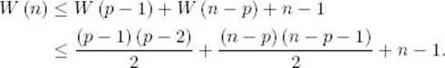
The last inequality is by the induction hypothesis. Algebraic manipulations can show that for 1 ≤ p ≤ n this last expression is

This completes the induction proof.

We have shown that the worst-case time complexity is given by

The worst case occurs when the array is already sorted because we always choose the first item for the pivot item. Therefore, if we have reason to believe that the array is close to being sorted, this is not a good choice for the pivot item. When we discuss Quicksort further in Chapter 7, we will investigate other methods for choosing the pivot item. If we use these methods, the worst case does not occur when the array is already sorted. But the worst-case time complexity is still n (n − 1) /2.

In the worst case, Algorithm 2.6 is no faster than Exchange Sort (Algorithm 1.3). Why then is this sort called Quicksort? As we shall see, it is in its average-case behavior that Quicksort earns its name.

Analysis of Algorithm 2.6

Average-Case Time Complexity (Quicksort)

Basic operation: the comparison of S [i] with pivotitem in partition

Input size: n, the number of items in the array S.

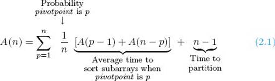
We will assume that we have no reason to believe that the numbers in the array are in any particular order, and therefore that the value of pivotpoint returned by partition is equally likely to be any of the numbers from 1 through n. If there was reason to believe a different distribution, this analysis would not be applicable. The average obtained is, therefore, the average sorting time when every possible ordering is sorted the same number of times. In this case, the average-case time complexity is given by the following recurrence:

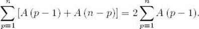
In the exercises we show that

Plugging this equality into Equality 2.1 yields

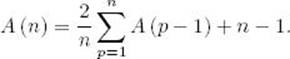
Multiplying by n we have

Applying Equality 2.2 to n − 1 gives

Subtracting Equality 2.3 from Equality 2.2 yields

which simplifies to

If we let

we have the recurrence

Like the recurrence in Example B.22 in Appendix B, the approximate solution to this recurrence is given by

which implies that

Quicksort’s average-case time complexity is of the same order as Mergesort’s time complexity. Mergesort and Quicksort are compared further in Chapter 7 and in Knuth (1973).

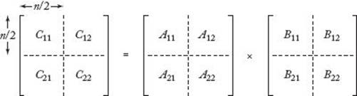
2.5 Strassen’s Matrix Multiplication Algorithm

Recall that Algorithm 1.4 (Matrix Multiplication) multiplied two matrices strictly according to the definition of matrix multiplication. We showed that the time complexity of its number of multiplications is given by T(n) = n³, where n is the number of rows and columns in the matrices. We can also analyze the number of additions. As you will show in the exercises, after the algorithm is modified slightly, the time complexity of the number of additions is given by T(n) = n³ − n². Because both of these time complexities are in Θ(n³), the algorithm can become impractical fairly quickly. In 1969, Strassen published an algorithm whose time complexity is better than cubic in terms of both multiplications and additions/subtractions. The following example illustrates his method.

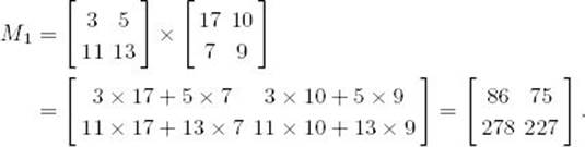
Example 2.4

Suppose we want the product C of two 2 × 2 matrices, A and B. That is,

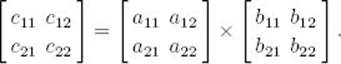
Strassen determined that if we let

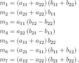
the product C is given by

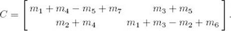
In the exercises, you will show that this is correct.

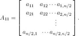
To multiply two 2 × 2 matrices, Strassen’s method requires seven multiplications and 18 additions/subtractions, whereas the straightforward method requires eight multiplications and four additions/subtractions. We have saved ourselves one multiplication at the expense of doing 14 additional additions or subtractions. This is not very impressive, and indeed it is not in the case of 2 × 2 matrices that Strassen’s method is of value. Because the commutativity of multiplications is not used in Strassen’s formulas, those formulas pertain to larger matrices that are each divided into four submatrices. First we divide the matrices A and B, as illustrated in Figure 2.4. Assuming that n is a power of 2, the matrix A₁₁, for example, is meant to represent the following submatrix of A:

Using Strassen’s method, first we compute

where our operations are now matrix addition and multiplication. In the same way, we compute M₂ through M₇. Next we compute

and C₁₂, C₂₁, and C₂₂. Finally, the product C of A and B is obtained by combining the four submatrices C_ij. The following example illustrates these steps.

Figure 2.4 The partitioning into submatrices in Strassen’s algorithm.

Example 2.5

Suppose that

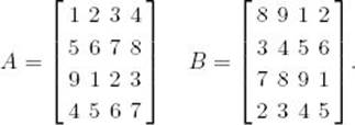
Figure 2.5 illustrates the partitioning in Strassen’s method. The computations proceed as follows:

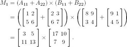
Figure 2.5 The partitioning in Strassen’s algorithm with n = 4 and values given to the matrices.

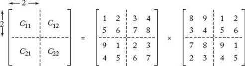
When the matrices are sufficiently small, we multiply in the standard way. In this example, we do this when n = 2. Therefore,

After this, M₂ through M₇ are computed in the same way, and then the values of C₁₁, C₁₂, C₂₁, and C₂₂ are computed. They are combined to yield C.

Next we present an algorithm for Strassen’s method when n is a power of 2.

Algorithm 2.8

Strassen

Problem: Determine the product of two n × n matrices where n is a power of 2.

Inputs: an integer n that is a power of 2, and two n × n matrices A and B.

Outputs: the product C of A and B.

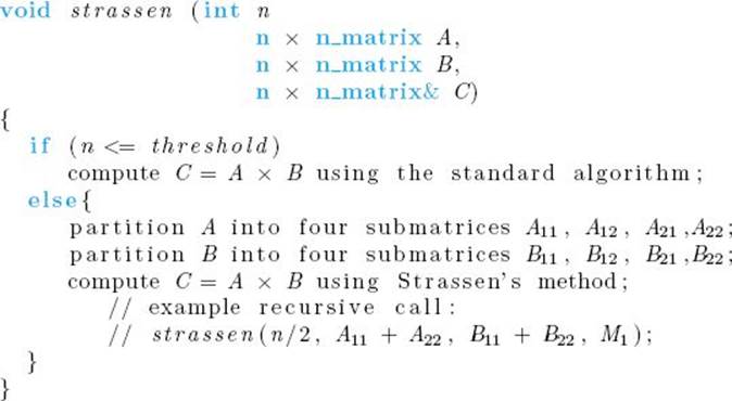
The value of threshold is the point at which we feel it is more efficient to use the standard algorithm than it would be to call procedure strassen recursively. In Section 2.7 we discuss a method for determining thresholds.

Analysis of Algorithm 2.8

Every-Case Time Complexity Analysis of Number of Multiplications (Strassen)

Basic operation: one elementary multiplication.

Input size: n, the number of rows and columns in the matrices.

For simplicity, we analyze the case in which we keep dividing until we have two 1 × 1 matrices, at which point we simply multiply the numbers in each matrix. The actual threshold value used does not affect the order. When n = 1, exactly one multiplication is done. When we have two n × nmatrices with n > 1, the algorithm is called exactly seven times with an (n/2) × (n/2) matrix passed each time, and no multiplications are done at the top level. We have established the recurrence

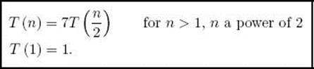
This recurrence is solved in Example B.2 in Appendix B. The solution is

Analysis of Algorithm 2.8

Every-Case Time Complexity Analysis of Number of Additions/Subtractions (Strassen)

Basic operation: one elementary addition or subtraction.

Input size: n, the number of rows and columns in the matrices.

Again we assume that we keep dividing until we have two 1 × 1 matrices. When n = 1, no additions/subtractions are done. When we have two n × n matrices with n > 1, the algorithm is called exactly seven times with an (n/2) × (n/2) matrix passed in each time, and 18 matrix additions/subtractions are done on (n/2) × (n/2) matrices. When two (n/2) × (n/2) matrices are added or subtracted, (n/2)² additions or subtractions are done on the items in the matrices. We have established the recurrence

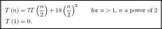
This recurrence is solved in Example B.20 in Appendix B. The solution is

When n is not a power of 2, we must modify the previous algorithm. One simple modification is to add sufficient numbers of columns and rows of 0s to the original matrices to make the dimension a power of 2. Alternatively, in the recursive calls we could add just one extra row and one extra column of 0s whenever the number of rows and columns is odd. Strassen (1969) suggested the following, more complex modification. We embed the matrices in larger ones with 2^km rows and columns, where k = lg n − 4 and m = n/2^k + 1. We use Strassen’s method up to a threshold value ofm and use the standard algorithm after reaching the threshold. It can be shown that the total number of arithmetic operations (multiplications, additions, and subtractions) is less than 4.7n^2.81.

Table 2.3 compares the time complexities of the standard algorithm and Strassen’s algorithm for n a power of 2. If we ignore for the moment the overhead involved in the recursive calls, Strassen’s algorithm is always more efficient in terms of multiplications, and for large values of n, Strassen’s algorithm is more efficient in terms of additions/subtractions. In Section 2.7 we will discuss an analysis technique that accounts for the time taken by the recursive calls.

• Table 2.3A comparison of two algorithms that multiply n × n matrices

Shmuel Winograd developed a variant of Strassen’s algorithm that requires only 15 additions/subtractions. It appears in Brassard and Bratley (1988). For this algorithm, the time complexity of the additions/subtractions is given by

Coppersmith and Winograd (1987) developed a matrix multiplication algorithm whose time complexity for the number of multiplications is in O (n^2.38). However, the constant is so large that Strassen’s algorithm is usually more efficient.

It is possible to prove that matrix multiplication requires an algorithm whose time complexity is at least quadratic. Whether matrix multiplications can be done in quadratic time remains an open question; no one has ever created a quadratic-time algorithm for matrix multiplication, and no one has proven that it is not possible to create such an algorithm.

One last point is that other matrix operations such as inverting a matrix and finding the determinant of a matrix are directly related to matrix multiplication. Therefore, we can readily create algorithms for these operations that are as efficient as Strassen’s algorithm for matrix multiplication.

2.6 Arithmetic with Large Integers

Suppose that we need to do arithmetic operations on integers whose size exceeds the computer’s hardware capability of representing integers. If we need to maintain all the significant digits in our results, switching to a floating-point representation would be of no value. In such cases, our only alternative is to use software to represent and manipulate the integers. We can accomplish this with the help of the divide-and-conquer approach. Our discussion focuses on integers represented in base 10. However, the methods developed can be readily modified for use in other bases.

• 2.6.1 Representation of Large Integers: Addition and Other Linear-Time Operations

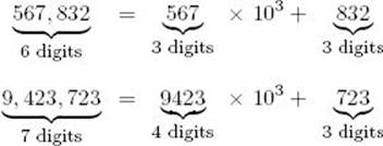
A straightforward way to represent a large integer is to use an array of integers, in which each array slot stores one digit. For example, the integer 543,127 can be represented in the array S as follows:

To represent both positive and negative integers we need only reserve the high-order array slot for the sign. We could use 0 in that slot to represent a positive integer and 1 to represent a negative integer. We will assume this representation and use the defined data type large integer to mean an array big enough to represent the integers in the application of interest.

It is not difficult to write linear-time algorithms for addition and subtraction, where n is the number of digits in the large integers. The basic operation consists of the manipulation of one decimal digit. In the exercises you are asked to write and analyze these algorithms. Furthermore, linear-time algorithms can readily be written that do the operation

where u represents a larger integer, m is a nonnegative integer, divide returns the quotient in integer division, and rem returns the remainder. This, too, is done in the exercises.

• 2.6.2 Multiplication of Large Integers

A simple quadratic-time algorithm for multiplying large integers is one that mimics the standard way learned in grammar school. We will develop one that is better than quadratic time. Our algorithm is based on using divide-and-conquer to split an n-digit integer into two integers of approximatelyn/2 digits. Following are two examples of such splits.

In general, if n is the number of digits in the integer u, we will split the integer into two integers, one with n/2 and the other with n/2, as follows:

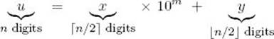
With this representation, the exponent m of 10 is given by

If we have two n-digit integers

their product is given by

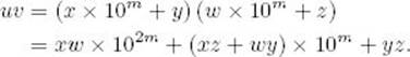
We can multiply u and v by doing four multiplications on integers with about half as many digits and performing linear-time operations. The following example illustrates this method.

Example 2.6

Consider the following:

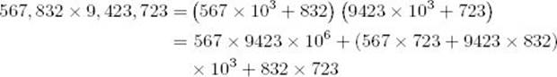
Recursively, these smaller integers can then be multiplied by dividing them into yet smaller integers. This division process is continued until a threshold value is reached, at which time the multiplication can be done in the standard way.

Although we illustrate the method using integers with about the same number of digits, it is still applicable when the number of digits is different. We simply use m = n/2 to split both of them, where n is the number of digits in the larger integer. The algorithm now follows. We keep dividing until one of the integers is 0 or we reach some threshold value for the larger integer, at which time the multiplication is done using the hardware of the computer (that is, in the usual way).

Algorithm 2.9

Large Integer Multiplication

Problem: Multiply two large integers, u and v.

Inputs: large integers u and v.

Outputs: prod, the product of u and v.

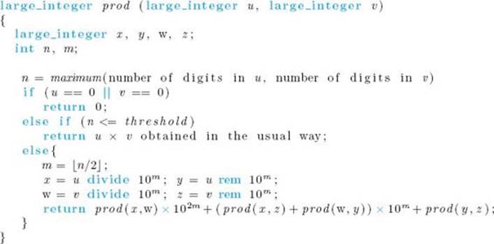
Notice that n is an implicit input to the algorithm because it is the number of digits in the larger of the two integers. Remember that divide, rem, and × represent linear-time functions that we need to write.

Analysis of Algorithm 2.9

Worst-Case Time Complexity (Large Integer Multiplication)

We analyze how long it takes to multiply two n-digit integers.

Basic operation: The manipulation of one decimal digit in a large integer when adding, subtracting, or doing divide 10^m, rem 10^m, or × 10^m. Each of these latter three calls results in the basic operation being done m times.

Input size: n, the number of digits in each of the two integers.

The worst case is when both integers have no digits equal to 0, because the recursion only ends when threshold is passed. We will analyze this case.

Suppose n is a power of 2. Then x, y, w, and z all have exactly n/2 digits, which means that the input size to each of the four recursive calls to prod is n/2. Because m = n/2, the linear-time operations of addition, subtraction, divide 10^m, rem 10^m, and × 10^m all have linear-time complexities in terms of n. The maximum input size to these linear-time operations is not the same for all of them, so the determination of the exact time complexity is not straightforward. It is much simpler to group all the linear-time operations in the one term cn, where c is a positive constant. Our recurrence is then

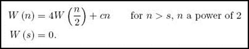
The actual value s at which we no longer divide the instance is less than or equal to threshold and is a power of 2, because all the inputs in this case are powers of 2.

For n not restricted to being a power of 2, it is possible to establish a recurrence like the previous one but involving floors and ceilings. Using an induction argument like the one in Example B.25 in Appendix B, we can show that W(n) is eventually nondecreasing. Therefore, Theorem B.6 inAppendix B implies that

Our algorithm for multiplying large integers is still quadratic. The problem is that the algorithm does four multiplications on integers with half as many digits as the original integers. If we can reduce the numbers of these multiplications, we can obtain an algorithm that is better than quadratic. We do this in the following way. Recall that function prod must determine

and we accomplished this by calling function prod recursively four times to compute

If instead we set

then

This means we can get the three values in Expression 2.4 by determining the following three values:

To get these three values we need to do only three multiplications, while doing some additional linear-time additions and subtractions. The algorithm that follows implements this method.

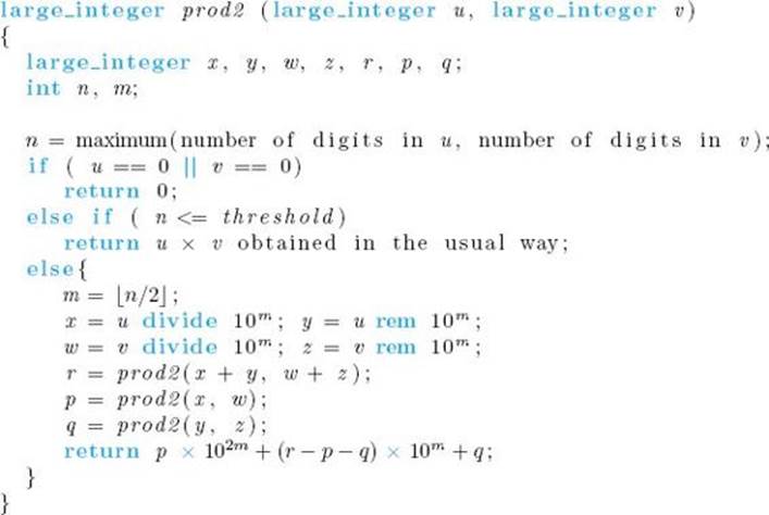
Algorithm 2.10

Large Integer Multiplication 2

Problem: Multiply two large integers, u and v.

Inputs: large integers u and v.

Outputs: prod2, the product of u and v.

Analysis of Algorithm 2.10

Worst-Case Time Complexity (Large Integer Multiplication 2)

We analyze how long it takes to multiply two n-digit integers.

Basic operation: The manipulation of one decimal digit in a large integer when adding, subtracting, or doing divide 10^m, rem 10^m, or × 10^m. Each of these latter three calls results in the basic operation being done m times.

Input size: n, the number of digits in each of the two integers.

The worst case happens when both integers have no digits equal to 0, because in this case the recursion ends only when the threshold is passed. We analyze this case.

• Table 2.4 Examples of the number of digits in x + y in Algorithm 2.10

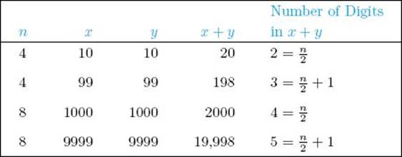
If n is a power of 2, then x, y, w, and z all have n/2 digits. Therefore, as Table 2.4 illustrates,

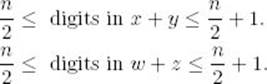
This means we can have the following input sizes for the given function calls:

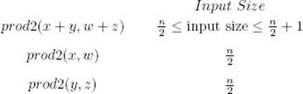
Because m = n/2, the linear-time operations of addition, subtraction, divide 10^m, rem 10^m, and × 10^m all have linear-time complexities in terms of n. Therefore, W(n) satisfies

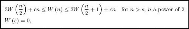
where s is less than or equal to threshold and is a power of 2, because all the inputs in this case are powers of 2. For n not restricted to being a power of 2, it is possible to establish a recurrence like the previous one but involving floors and ceilings. Using an induction argument like the one in Example B.25 in Appendix B, we can show that W(n) is eventually nondecreasing. Therefore, owing to the left inequality in this recurrence and Theorem B.6, we have

Next we show that

To that end, let

Using the right inequality in the recurrence, we have

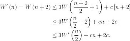
Because W(n) is nondecreasing, so is W′ (n). Therefore, owing to Theorem B.6 in Appendix B,

and so

Combining our two results, we have

Using Fast Fourier Transforms, Borodin and Munro (1975) developed a algorithm for multiplying large integers. The survey article (Brassard, Monet, and Zuffelatto, 1986) concerns very large integer multiplication.

It is possible to write algorithms for other operations on large integers, such as division and square root, whose time complexities are of the same order as that of the algorithm for multiplication.

2.7 Determining Thresholds

As discussed in Section 2.1, recursion requires a fair amount of overhead in terms of computer time. If, for example, we are sorting only eight keys, is it really worth this overhead just so we can use a Θ(n lg n) algorithm instead of a Θ(n²) algorithm? Or perhaps, for such a small n, would ExchangeSort (Algorithm 1.3) be faster than our recursive Mergesort? We develop a method that determines for what values of n it is at least as fast to call an alternative algorithm as it is to divide the instance further. These values depend on the divide-and-conquer algorithm, the alternative algorithm, and the computer on which they are implemented. Ideally, we would like to find an optimal threshold value of n. This would be an instance size such that for any smaller instance it would be at least as fast to call the other algorithm as it would be to divide the instance further, and for any larger instance size it would be faster to divide the instance again. However, as we shall see, an optimal threshold value does not always exist. Even if our analysis does not yield an optimal threshold value, we can use the results of the analysis to pick a threshold value. We then modify the divide-and-conquer algorithm so that the instance is no longer divided once n reaches that threshold value; instead, the alternative algorithm is called. We have already seen the use of thresholds in Algorithms 2.8, 2.9, and 2.10.

To determine a threshold, we must consider the computer on which the algorithm is implemented. This technique is illustrated using Mergesort and Exchange Sort. We use Mergesort’s worst-case time complexity in this analysis. So we are actually trying to optimize the worst-case behavior. When analyzing Mergesort, we determined that the worst case is given by the following recurrence:

Let’s assume that we are implementing Mergesort 2 (Algorithm 2.4). Suppose that on the computer of interest the time Mergesort 2 takes to divide and recombine an instance of size n is 32n µs, where µs stands for micro-seconds. The time to divide and recombine the instance includes the time to compute the value of mid, the time to do the stack operations for the two recursive calls, and the time to merge the two subarrays. Because there are several components to the division and recombination time, it is unlikely that the total time would simply be a constant times n. However, assume that this is the case to keep things as simple as possible. Because the term n − 1 in the recurrence for W(n) is the recombination time, it is included in the time 32n µs. Therefore, for this computer, we have

for Mergesort 2. Because only a terminal condition check is done when the input size is 1, we assume that W (1) is essentially 0. For simplicity, we initially limit our discussion to n being a power of 2. In this case we have the following recurrence:

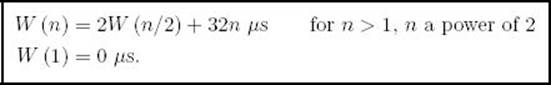
The techniques in Appendix B can be used to solve this recurrence. The solution is

Suppose that on this same computer Exchange Sort takes exactly

to sort an instance of size n. Sometimes students erroneously believe that the optimal point where Mergesort 2 should call Exchange Sort can now be found by solving the inequality

The solution is

Students sometimes believe that it is optimal to call Exchange Sort when n < 591 and to call Mergesort 2 otherwise. This analysis is only approximate because we base it on n being a power of 2. But more importantly it is incorrect, because it only tells us that if we use Mergesort 2 and keep dividing until n = 1, then Exchange Sort is better for n < 591. We want to use Mergesort 2 and keep dividing until it is better to call Exchange Sort, rather than divide the instance further. This is not the same as dividing until n = 1, and therefore the point at which we call Exchange Sort should be less than 591. That this value should be less than 591 is a bit hard to grasp in the abstract. The following concrete example, which determines the point at which it is more efficient to call Exchange Sort rather than dividing the instance further, should make the matter clear. From now on, we no longer limit our considerations to n being a power of 2.

Example 2.7

We determine the optimal threshold for Algorithm 2.5 (Mergesort 2) when calling Algorithm 1.3 (Exchange Sort). Suppose we modify Mergesort 2 so that Exchange Sort is called when n ≤ t for some threshold t. Assuming the hypothetical computer just discussed, for this version of Mergesort 2,

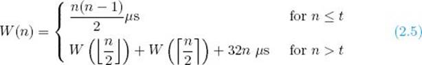
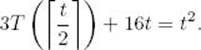
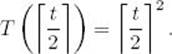
We want to determine the optimal value of t. That value is the value for which the top and bottom expressions in Equality 2.5 are equal, because this is the point where calling Exchange Sort is as efficient as dividing the instance further. Therefore, to determine the optimal value of t, we must solve

Because t/2 and t/2 are both less than or equal to t, the execution time is given by the top expression in Equality 2.5 if the instance has either of these input sizes. Therefore,

Substituting these equalities into Equation 2.6 yields

In general, in an equation with floors and ceilings, we can obtain a different solution when we insert an odd value for t than when we insert an even value for t. This is the reason there is not always an optimal threshold value. Such a case is investigated next. In this case, however, if we insert an even value for t, which is accomplished by setting t/2 and t/2 both equal to t/2, and solve Equation 2.7, we obtain

If we insert an odd value for t, which is accomplished by setting t/2 equal to (t − 1) /2 and t/2 equal to (t + 1) /2 and solve Equation 2.7, we obtain

Therefore, we have an optimal threshold value of 128.

Next we give an example where there is no optimal threshold value.

Example 2.8

Suppose for a given divide-and-conquer algorithm running on a particular computer we determine that

where 16n µs is the time needed to divide and recombine an instance of size n. Suppose on the same computer a certain iterative algorithm takes n² µs to process an instance of size n. To determine the value t at which we should call the iterative algorithm, we need to solve

Because t/2 ≤ t, the iterative algorithm is called when the input has this size, which means that

Therefore, we need to solve

If we substitute an even value for t (by setting t/2 = t/2) and solve, we get

If we substitute an odd value for t (by setting t/2 = (t + 1) /2) and solve, we get

Because the two values of t are not equal, there is no optimal threshold value. This means that if the size of an instance is an even integer between 64 and 70, it is more efficient to divide the instance one more time, whereas if the size is an odd integer between 64 and 70, it is more efficient to call the iterative algorithm. When the size is less than 64, it is always more efficient to call the iterative algorithm. When the size is greater than 70, it is always more efficient to divide the instance again. Table 2.5 illustrates that this is so.

• Table 2.5 Various instance sizes illustrating that the threshold is 64 for n even and 70 for n odd in Example 2.8

2.8 When Not to Use Divide-and-Conquer

If possible, we should avoid divide-and-conquer in the following two cases:

1. An instance of size n is divided into two or more instances each almost of size n.

2. An instance of size n is divided into almost n instances of size n/c, where c is a constant.

The first partitioning leads to an exponential-time algorithm, where the second leads to a n^{Θ(lg n)} algorithm. Neither of these is acceptable for large values of n. Intuitively, we can see why such partitionings lead to poor performance. For example, the first case would be like Napoleon dividing an opposing army of 30,000 soldiers into two armies of 29,999 soldiers (if this were somehow possible). Rather than dividing his enemy, he has almost doubled their number! If Napoleon did this, he would have met his Waterloo much sooner.

As you should now verify, Algorithm 1.6 (nth Fibonacci Term, Recursive) is a divide-and-conquer algorithm that divides the instance that computes the nth term into two instances that compute respectively the (n − 1)st term and the (n − 2)nd term. Although n is not the input size in that algorithm, the situation is the same as that just described concerning input size.

That is, the number of terms computed by Algorithm 1.6 is exponential in n, whereas the number of terms computed by Algorithm 1.7 (nth Fibonacci Term, Iterative) is linear in n.

Sometimes, on the other hand, a problem requires exponentiality, and in such a case there is no reason to avoid the simple divide-and-conquer solution. Consider the Towers of Hanoi problem, which is presented in Exercise 17. Briefly, the problem involves moving n disks from one peg to another given certain restrictions on how they may be moved. In the exercises you will show that the sequence of moves, obtained from the standard divide-and-conquer algorithm for the problem, is exponential in terms of n and that it is the most efficient sequence of moves given the problem’s restrictions. Therefore, the problem requires an exponentially large number of moves in terms of n.

EXERCISES

Sections 2.1

1. Use Binary Search, Recursive (Algorithm 2.1) to search for the integer 120 in the following list (array) of integers. Show the actions step by step.

2. Suppose that, even unrealistically, we are to search a list of 700 million items using Binary Search, Recursive (Algorithm 2.1). What is the maximum number of comparisons that this algorithm must perform before finding a given item or concluding that it is not in the list?

3. Let us assume that we always perform a successful search. That is, in Algorithm 2.1 the item x can always be found in the list S. Improve Algorithm 2.1 by removing all unnecessary operations.

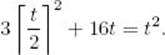
4. Show that the worst-case time complexity for Binary Search (Algorithm 2.1) is given by

when n is not restricted to being a power of 2. Hint: First show that the recurrence equation for W(n) is given by

To do this, consider even and odd values of n separately. Then use induction to solve the recurrence equation.

5. Suppose that, in Algorithm 2.1 (line 4), the splitting function is changed to mid = low;. Explain the new search strategy. Analyze the performance of this strategy and show the results using order notation.

6. Write an algorithm that searches a sorted list of n items by dividing it into three sublists of almost n/3 items. This algorithm finds the sublist that might contain the given item and divides it into three smaller sublists of almost equal size. The algorithm repeats this process until it finds the item or concludes that the item is not in the list. Analyze your algorithm and give the results using order notation.

7. Use the divide-and-conquer approach to write an algorithm that finds the largest item in a list of n items. Analyze your algorithm, and show the results in order notation.

Sections 2.2

8. Use Mergesort (Algorithms 2.2 and 2.4) to sort the following list. Show the actions step by step.

9. Give the tree of recursive calls in Exercise 8.

10. Write for the following problem a recursive algorithm whose worst-case time complexity is not worse than Θ(n ln n). Given a list of n distinct positive integers, partition the list into two sublists, each of size n/2, such that the difference between the sums of the integers in the two sublists is maximized. You may assume that n is a multiple of 2.

11. Write a nonrecursive algorithm for Mergesort (Algorithms 2.2 and 2.4).

12. Show that the recurrence equation for the worst-case time complexity for Mergesort (Algorithms 2.2 and 2.4) is given by

when n is not restricted to being a power of 2.

13. Write an algorithm that sorts a list of n items by dividing it into three sublists of about n/3 items, sorting each sublist recursively and merging the three sorted sublists. Analyze your algorithm, and give the results under order notation.

Sections 2.3

14. Given the recurrence relation

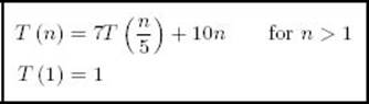
find T(625).

15. Consider algorithm solve given below. This algorithm solves problem P by finding the output (solution) O corresponding to any input I.

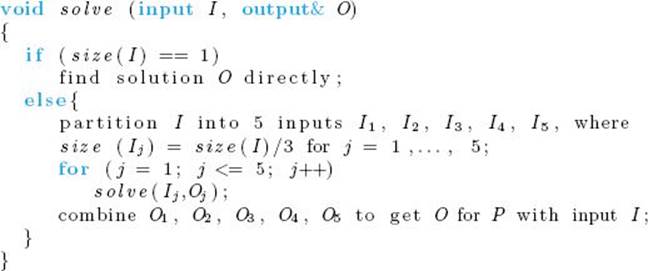
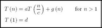
Assume g (n) basic operations for partitioning and combining and no basic operations for an instance of size 1.

(a) Write a recurrence equation T(n) for the number of basic operations needed to solve P when the input size is n.

(b) What is the solution to this recurrence equation if g (n) ∈ Θ(n)? (Proof is not required.)

(c) Assuming that g (n) = n², solve the recurrence equation exactly for n = 27.

(d) Find the general solution for n a power of 3.

16. Suppose that, in a divide-and-conquer algorithm, we always divide an instance of size n of a problem into 10 subinstances of size n/3, and the dividing and combining steps take a time in Θ(n²) _. Write a recurrence equation for the running time T(n), and solve the equation for T(n).

17. Write a divide-and-conquer algorithm for the Towers of Hanoi problem. The Towers of Hanoi problem consists of three pegs and n disks of different sizes. The object is to move the disks that are stacked, in decreasing order of their size, on one of the three pegs to a new peg using the third one as a temporary peg. The problem should be solved according to the following rules: (1) when a disk is moved, it must be placed on one of the three pegs; (2) only one disk may be moved at a time, and it must be the top disk on one of the pegs; and (3) a larger disk may never be placed on top of a smaller disk.

(a) Show for your algorithm that S (n) = 2ⁿ − 1. (Here S (n) denotes the number of steps (moves), given an input of n disks.)

(b) Prove that any other algorithm takes at least as many moves as given in part (a).

18. When a divide-and-conquer algorithm divides an instance of size n of a problem into subinstances each of size n/c, the recurrence relation is typically given by

where g (n) is the cost of the dividing and combining processes, and d is a constant. Let n = c^k.

(a) Show that

(b) Solve the recurrence relation given that g(n) ∈ Θ(n).

Sections 2.4

19. Use Quicksort (Algorithm 2.6) to sort the following list. Show the actions step by step.

20. Give the tree of recursive calls in Exercise 19.

21. Show that if

then

This result is used in the discussion of the worst-case time complexity analysis of Algorithm 2.6 (Quicksort).

22. Verify the following identity

This result is used in the discussion of the average-case time complexity analysis of Algorithm 2.6 (Quicksort).

23. Write a nonrecursive algorithm for Quicksort (Algorithm 2.6). Analyze your algorithm, and give the results using order notation.

24. Assuming that Quicksort uses the first item in the list as the pivot item:

(a) Give a list of n items (for example, an array of 10 integers) representing the worst-case scenario.

(b) Give a list of n items (for example, an array of 10 integers) representing the best-case scenario.

Sections 2.5

25 Show that the number of additions performed by Algorithm 1.4 (Matrix Multiplication) can be reduced to n³ − n² after a slight modification of this algorithm.

26. In Example 2.4, we gave Strassen’s product of two 2 × 2 matrices. Verify the correctness of this product.

27. How many multiplications would be performed in finding the product of two 64 × 64 matrices using the standard algorithm?

28. How many multiplications would be performed in finding the product of two 64 × 64 matrices using Strassen’s method (Algorithm 2.8)?

29. Write a recurrence equation for the modified Strassen’s algorithm developed by Shmuel Winograd that uses 15 additions/subtractions instead of 18. Solve the recurrence equation, and verify your answer using the time complexity shown at the end of Section 2.5.

Sections 2.6

30. Use Algorithm 2.10 (Large Integer Multiplication 2) to find the product of 1253 and 23,103.

31. How many multiplications are needed to find the product of the two integers in Exercise 30?

32. Write algorithms that perform the operations

where u represents a large integer, m is a nonnegative integer, divide returns the quotient in integer division, and rem returns the remainder. Analyze your algorithms, and show that these operations can be done in linear time.

33. Modify Algorithm 2.9 (Large Integer Multiplication) so that it divides each n-digit integer into

(a) three smaller integers of n/3 digits (you may assume that n = 3^k).

(b) four smaller integers of n/4 digits (you may assume that n = 4^k).

Analyze your algorithms, and show their time complexities in order notation.

Sections 2.7

34. Implement both Exchange Sort and Quicksort algorithms on your computer to sort a list of n elements. Find the lower bound for n that justifies application of the Quicksort algorithm with its overhead.

35. Implement both the standard algorithm and Strassen’s algorithm on your computer to multiply two n × n matrices (n = 2^k). Find the lower bound for n that justifies application of Strassen’s algorithm with its overhead.

36. Suppose that on a particular computer it takes 12n² µs to decompose and recombine an instance of size n in the case of Algorithm 2.8 (Strassen). Note that this time includes the time it takes to do all the additions and subtractions. If it takes n³ µs to multiply two n × n matrices using the standard algorithm, determine thresholds at which we should call the standard algorithm instead of dividing the instance further. Is there a unique optimal threshold?

Sections 2.8

37. Use the divide-and-conquer approach to write a recursive algorithm that computes n!. Define the input size (see Exercise 36 in Chapter 1), and answer the following questions. Does your function have an exponential time complexity? Does this violate the statement of case 1 given in Section 2.8?

38. Suppose that, in a divide-and-conquer algorithm, we always divide an instance of size n of a problem into n subinstances of size n/3, and the dividing and combining steps take linear time. Write a recurrence equation for the running time T(n), and solve this recurrence equation for T(n). Show your solution in order notation.

Additional Exercises

39. Implement both algorithms for the Fibonacci Sequence (Algorithms 1.6 and

1.7). Test each algorithm to verify that it is correct. Determine the largest number that the recursive algorithm can accept as its argument and still compute the answer within 60 seconds. See how long it takes the iterative algorithm to compute this answer.

40. Write an efficient algorithm that searches for a value in an n × m table (two-dimensional array). This table is sorted along the rows and columns—that is,

41. Suppose that there are n = 2^k teams in an elimination tournament, in which there are n/2 games in the first round, with the n/2 = 2^k−1 winners playing in the second round, and so on.

(a) Develop a recurrence equation for the number of rounds in the tournament.

(b) How many rounds are there in the tournament when there are 64 teams?

(c) Solve the recurrence equation of part (a).

42. A tromino is a group of three unit squares arranged in an L-shape. Consider the following tiling problem: The input is an m × m array of unit squares where m is a positive power of 2, with one forbidden square on the array. The output is a tiling of the array that satisfies the following conditions:

Every unit square other than the input square is covered by a tromino.

No tromino covers the input square.

No two trominos overlap.

No tromino extends beyond the board.

Write a divide-and-conquer algorithm that solves this problem.

43. Consider the following problem:

(a) Suppose we have nine identical-looking coins numbered 1 through 9 and only one of the coins is heavier than the others. Suppose further that you have one balance scale and are allowed only two weighings. Develop a method for finding the heavier counterfeit coin given these constraints.

(b) Suppose we now have an integer n (that represents n coins) and only one of the coins is heavier than the others. Suppose further that n is a power of 3 and you are allowed log₃ n weighings to determine the heavier coin. Write an algorithm that solves this problem. Determine the time complexity of your algorithm.

44. Write a recursive Θ(n lg n) algorithm whose parameters are three integers x, n, and p, and which computes the remainder when xⁿ is divided by p. For simplicity, you may assume that n is a power of 2—that is, that n = 2^k for some positive integer k.

45. Use the divide-and-conquer approach to write a recursive algorithm that finds the maximum sum in any contiguous sublist of a given list of n real values. Analyze your algorithm, and show the results in order notation.