Foundations of Algorithms (2015)

Chapter 3 Dynamic Programming

Recall that the number of terms computed by the divide-and-conquer algorithm for determining the nth Fibonacci term (Algorithm 1.6) is exponential in n. The reason is that the divide-and-conquer approach solves an instance of a problem by dividing it into smaller instances and then blindly solving these smaller instances. As discussed in Chapter 2, this is a top-down approach. It works in problems such as Mergesort, where the smaller instances are unrelated. They are unrelated because each consists of an array of keys that must be sorted independently. However, in problems such as the nth Fibonacci term, the smaller instances are related. For example, as shown in Section 1.2, to compute the fifth Fibonacci term we need to compute the fourth and third Fibonacci terms. However, the determinations of the fourth and third Fibonacci terms are related in that they both require the second Fibonacci term. Because the divide-and-conquer algorithm makes these two determinations independently, it ends up computing the second Fibonacci term more than once. In problems where the smaller instances are related, a divide-and-conquer algorithm often ends up repeatedly solving common instances, and the result is a very inefficient algorithm.

Dynamic programming, the technique discussed in this chapter, takes the opposite approach. Dynamic programming is similar to divide-and-conquer in that an instance of a problem is divided into smaller instances. However, in this approach we solve small instances first, store the results, and later, whenever we need a result, look it up instead of recomputing it. The term “dynamic programming” comes from control theory, and in this sense “programming” means the use of an array (table) in which a solution is constructed. As mentioned in Chapter 1, our efficient algorithm (Algorithm 1.7) for computing the nth Fibonacci term is an example of dynamic programming. Recall that this algorithm determines the nth Fibonacci term by constructing in sequence the first n+1 terms in an array f indexed from 0 to n. In a dynamic programming algorithm, we construct a solution from the bottom up in an array (or sequence of arrays). Dynamic programming is therefore a bottom-up approach. Sometimes, as in the case for Algorithm 1.7, after developing the algorithm using an array (or sequence of arrays), we are able to revise the algorithm so that much of the originally allocated space is not needed.

The steps in the development of a dynamic programming algorithm are as follows:

1. Establish a recursive property that gives the solution to an instance of the problem.

2. Solve an instance of the problem in a bottom-up fashion by solving smaller instances first.

To illustrate these steps, we present another simple example of dynamic programming in Section 3.1. The remaining sections present more advanced applications of dynamic programming.

3.1 The Binomial Coefficient

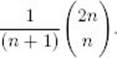
The binomial coefficient, which is discussed in Section A.7 in Appendix A, is given by

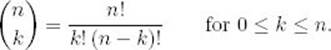
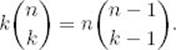
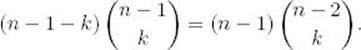
For values of n and k that are not small, we cannot compute the binomial coefficient directly from this definition because n! is very large even for moderate values of n. In the exercises we establish that

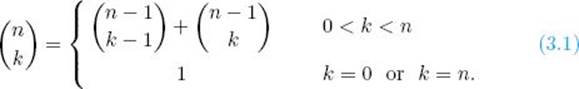
We can eliminate the need to compute n! or k! by using this recursive property. This suggests the following divide-and-conquer algorithm.

Algorithm 3.1

Binomial Coefficient Using Divide-and-Conquer

Problem: Compute the binomial coefficient.

Inputs: nonnegative integers n and k, where k ≤ n.

Outputs: bin, the binomial coefficient

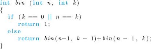
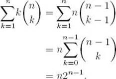
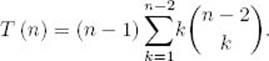
Like Algorithm 1.6 (nth Fibonacci Term, Recursive), this algorithm is very inefficient. In the exercises you will establish that the algorithm computes

terms to determine The problem is that the same instances are solved in each recursive call. For example, bin (n − 1, k − 1) and bin (n − 1, k) both need the result of bin (n − 2, k − 1), and this instance is solved separately in each recursive call. As mentioned in Section 2.8, the divide-and-conquer approach is always inefficient when an instance is divided into two smaller instances that are almost as large as the original instance.

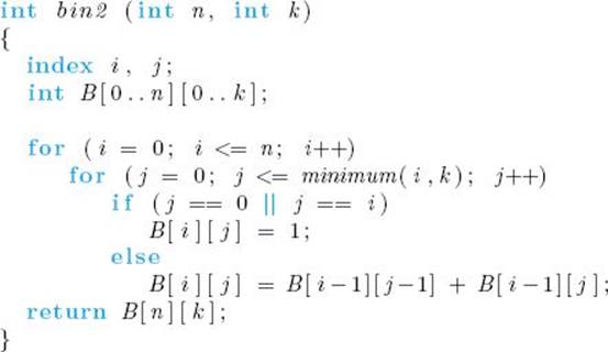
A more efficient algorithm is developed next using dynamic programming. A recursive property has already been established in Equality 3.1. We will use that property to construct our solution in an array B, where B [i] [j] will contain The steps for constructing a dynamic programming algorithm for this problem are as follows:

1. Establish a recursive property. This has already been done in Equality 3.1. Written in terms of B, it is

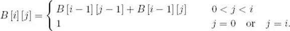
2. Solve an instance of the problem in a bottom-up fashion by computing the rows in B in sequence starting with the first row.

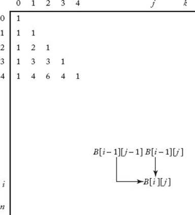
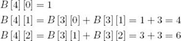
Step 2 is illustrated in Figure 3.1. (You may recognize the array in that figure as Pascal’s triangle.) Each successive row is computed from the row preceding it using the recursive property established in Step 1. The final value computed, B [n] [k], is Example 3.1 illustrates these steps. Notice in the example that we compute only the first two columns. The reason is that k = 2 in the example, and in general we need to compute the values in each row only up to the kth column. Example 3.1 computes B [0] [0] because the binomial coefficient is defined for n = k = 0. Therefore, an algorithm would perform this step even though the value is not needed in the computation of other binomial coefficients.

Figure 3.1 The array B used to compute the binomial coefficient.

Example 3.1

Compute B [4] [2] =

Compute row 0: {This is done only to mimic the algorithm exactly.}

{The value B [0] [0] is not needed in a later computation.}

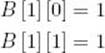
Compute row 1:

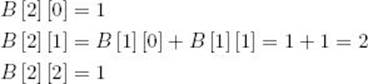
Compute row 2:

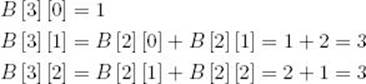
Compute row 3:

Compute row 4:

Example 3.1 computes increasingly larger values of the binomial coefficient in sequence. At each iteration, the values needed for that iteration have already been computed and saved. This procedure is fundamental to the dynamic programming approach. The following algorithm implements this approach in computing the binomial coefficient.

Algorithm 3.2

Binomial Coefficient Using Dynamic Programming

Problem: Compute the binomial coefficient.

Inputs: nonnegative integers n and k, where k ≤ n.

Outputs: bin2, the binomial coefficient

The parameters n and k are not the size of the input to this algorithm. Rather, they are the input, and the input size is the number of symbols it takes to encode them. We discussed a similar situation in Section 1.3 regarding algorithms that compute the nth Fibonacci term. However, we can still gain insight into the efficiency of the algorithm by determining how much work it does as a function for n and k. For given n and k, let’s compute the number of passes through the for-j loop. The following table shows the number of passes for each value of i:

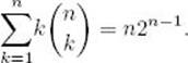
The total number of passes is therefore given by

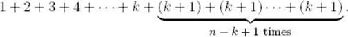
Applying the result in Example A.1 in Appendix A, we find that this expression equals

By using dynamic programming instead of divide-and-conquer, we have developed a much more efficient algorithm. As mentioned earlier, dynamic programming is similar to divide-and-conquer in that we find a recursive property that divides an instance into smaller instances. The difference is that in dynamic programming we use the recursive property to iteratively solve the instances in sequence, starting with the smallest instance, instead of blindly using recursion. In this way we solve each smaller instance just once. Dynamic programming is a good technique to try when divide-and-conquer leads to an inefficient algorithm.

The most straightforward way to present Algorithm 3.2 was to create the entire two-dimensional array B. However, once a row is computed, we no longer need the values in the row that precedes it. Therefore, the algorithm can be written using only a one-dimensional array indexed from 0 to k. This modification is investigated in the exercises. Another improvement to the algorithm would be to take advantage of the fact that

3.2 Floyd’s Algorithm for Shortest Paths

A common problem encountered by air travelers is the determination of the shortest way to fly from one city to another when a direct flight does not exist. Next we develop an algorithm that solves this and similar problems. First, let’s informally review some graph theory. Figure 3.2 shows a weighted, directed graph. Recall that in a pictorial representation of a graph the circles represent vertices, and a line from one circle to another represents an edge (also called an arc). If each edge has a direction associated with it, the graph is called a directed graph or digraph. When drawing an edge in such a graph, we use an arrow to show the direction. In a digraph there can be two edges between two vertices, one going in each direction. For example, in Figure 3.2 there is an edge from v₁ to v₂ and an edge from v₂ to v₁. If the edges have values associated with them, the values are called weights and the graph is called a weighted graph. We assume here that these weights are nonnegative. Although the values are ordinarily called weights, in many applications they represent distances. Therefore, we talk of a path from one vertex to another. In a directed graph, a path is a sequence of vertices such that there is an edge from each vertex to its successor. For example, in Figure 3.2 the sequence [v₁, v₄, v₃] is a path because there is an edge from v₁ to v₄ and an edge from v₄ to v₃. The sequence [v₃, v₄, v₁] is not a path because there is no edge from v₄ to v₁. A path from a vertex to itself is called a cycle. The path [v₁, v₄, v₅, v₁] in Figure 3.2 is a cycle. If a graph contains a cycle, it is cyclic; otherwise, it is acyclic. A path is called simple if it never passes through the same vertex twice. The path [v₁, v₂, v₃] in Figure 3.2 is simple, but the path [v₁, v₄, v₅, v₁, v₂] is not simple. Notice that a simple path never contains a subpath that is a cycle. The length of a path in a weighted graph is the sum of the weights on the path; in an unweighted graph it is simply the number of edges in the path.

Figure 3.2 A weighted, directed graph.

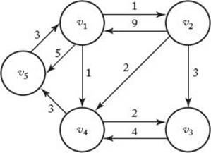
A problem that has many applications is finding the shortest paths from each vertex to all other vertices. Clearly, a shortest path must be a simple path. In Figure 3.2 there are three simple paths from v₁ to v₃—namely [v₁, v₂, v₃], [v₁, v₄, v₃], and [v₁, v₂, v₄, v₃]. Because [v₁, v₄, v₃] is the shortest path from v₁ to v₃. As mentioned previously, one common application of shortest paths is determining the shortest routes between cities.

The Shortest Paths problem is an optimization problem. There can be more than one candidate solution to an instance of an optimization problem. Each candidate solution has a value associated with it, and a solution to the instance is any candidate solution that has an optimal value. Depending on the problem, the optimal value is either the minimum or the maximum. In the case of the Shortest Paths problem, a candidate solution is a path from one vertex to another, the value is the length of the path, and the optimal value is the minimum of these lengths.

Because there can be more than one shortest path from one vertex to another, our problem is to find any one of the shortest paths. An obvious algorithm for this problem would be to determine, for each vertex, the lengths of all the paths from that vertex to each other vertex, and to compute the minimum of these lengths. However, this algorithm is worse than exponential-time. For example, suppose there is an edge from every vertex to every other vertex. Then a subset of all the paths from one vertex to another vertex is the set of all those paths that start at the first vertex, end at the other vertex, and pass through all the other vertices. Because the second vertex on such a path can be any of n − 2 vertices, the third vertex on such a path can be any of n − 3 vertices, … , and the second-to-last vertex on such a path can be only one vertex, the total number of paths from one vertex to another vertex that pass through all the other vertices is

which is worse than exponential. We encounter this same situation in many optimization problems. That is, the obvious algorithm that considers all possibilities is exponential-time or worse. Our goal is to find a more efficient algorithm.

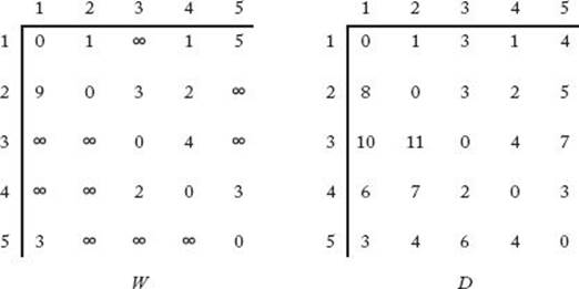
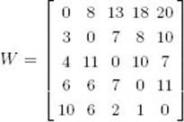
Using dynamic programming, we create a cubic-time algorithm for the Shortest Paths problem. First we develop an algorithm that determines only the lengths of the shortest paths. After that we modify it to produce shortest paths as well. We represent a weighted graph containing n vertices by an array W where

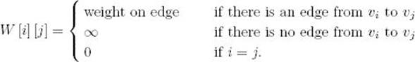
Because vertex v_j is said to be adjacent to v_i if there is an edge from v_i to v_j, this array is called the adjacency matrix representation of the graph. The graph in Figure 3.2 is represented in this manner in Figure 3.3. The array D in Figure 3.3 contains the lengths of the shortest paths in the graph. For example, D [3] [5] is 7 because 7 is the length of a shortest path from v₃ to v₅. If we can develop a way to calculate the values in D from those in W, we will have an algorithm for the Shortest Paths problem. We accomplish this by creating a sequence of n+1 arrays D^(k), where 0 ≤ k ≤ n and where

Figure 3.3 W represents the graph in Figure 3.2 and D contains the lengths of the shortest paths. Our algorithm for the Shortest Paths problem computes the values in D from those in W.

D^(k) [i] [j] = length of a shortest path from v_i to v_j using only vertices in the set {v₁, v₂, … , v_k} as intermediate vertices.

Before showing why this enables us to compute D from W, let’s illustrate the meaning of the items in these arrays.

Example 3.2

We will calculate some exemplary values of D^(k) [i] [j] for the graph in Figure 3.2.

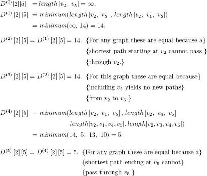
The last value computed, D⁽⁵⁾ [2] [5], is the length of a shortest path from v₂ to v₅ that is allowed to pass through any of the other vertices. This means that it is the length of a shortest path.

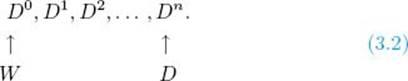
Because D⁽ⁿ⁾ [i] [j] is the length of a shortest path from v_i to v_j that is allowed to pass through any of the other vertices, it is the length of a shortest path from v_i to v_j. Because D⁽⁰⁾ [i] [j] is the length of a shortest path that is not allowed to pass through any other vertices, it is the weight on the edge from v₁ to v_j. We have established that

Therefore, to determine D from W we need only find a way to obtain D⁽ⁿ⁾ from D⁽⁰⁾. The steps for using dynamic programming to accomplish this are as follows:

1. Establish a recursive property (process) with which we can compute D^(k) from D^(k−1).

2. Solve an instance of the problem in a bottom-up fashion by repeating the process (established in Step 1) for k = 1 to n. This creates the sequence

We accomplish Step 1 by considering two cases:

Case 1. At least one shortest path from v_i to v_j, using only vertices in {v₁, v₂, … , v_k} as intermediate vertices, does not use v_k. Then

An example of this case in Figure 3.2 is that

because when we include vertex v₅, the shortest path from v₁ to v₃ is still [v₁, v₄, v₃].

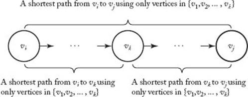
Case 2. All shortest paths from v_i to v_j, using only vertices in {v₁, v₂, … , v_k} as intermediate vertices, do use v_k. In this case any shortest path appears as in Figure 3.4. Because v_k cannot be an intermediate vertex on the subpath from v_i to v_k, that subpath uses only vertices in {v₁, v₂, … , v_k−1} as intermediates. This implies that the subpath’s length must be equal to D^(k−1) [i] [k] for the following reasons: First, the subpath’s length cannot be shorter because D^(k−1) [i] [k] is the length of a shortest path from v₁ to v_k using only vertices in {v₁, v₂, … , v_k−1} as intermediates. Second, the subpath’s length cannot be longer because if it were, we could replace it in Figure 3.4 by a shortest path, which contradicts the fact that the entire path in Figure 3.4 is a shortest path. Similarly, the length of the subpath from v_k to v_j in Figure 3.4 must be equal to D^(k−1) [k] [j]. Therefore, in the second case

Figure 3.4 The shortest path uses v_k.

An example of the second case in Figure 3.2 is that

Because we must have either Case 1 or Case 2, the value of D^(k) [i] [j] is the minimum of the values on the right in Equalities 3.3 and 3.4. This means that we can determine D^(k) from D^(k−1) as follows:

We have accomplished Step 1 in the development of a dynamic programming algorithm. To accomplish Step 2, we use the recursive property in Step 1 to create the sequence of arrays shown in Expression 3.2. Let’s do an example showing how each of these arrays is computed from the previous one.

Example 3.3

Given the graph in Figure 3.2, which is represented by the adjacency matrix W in Figure 3.3, some sample computations are as follows (recall that D⁽⁰⁾ = W):

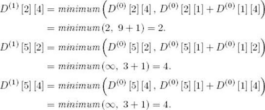
Once the whole array D⁽¹⁾ is computed, the array D⁽²⁾ is computed. A sample computation is

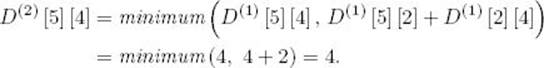
After computing all of D⁽²⁾, we continue in sequence until D⁽⁵⁾ is computed. This final array is D, the lengths of the shortest paths. It appears on the right in Figure 3.3.

Next we present the algorithm developed by Floyd (1962) and known as Floyd’s algorithm. Following the algorithm, we explain why it uses only one array D besides the input array W.

Algorithm 3.3

Floyd’s Algorithm for Shortest Paths

Problem: Compute the shortest paths from each vertex in a weighted graph to each of the other vertices. The weights are nonnegative numbers.

Inputs: A weighted, directed graph and n, the number of vertices in the graph. The graph is represented by a two-dimensional array W, which has both its rows and columns indexed from 1 to n, where W [i] [j] is the weight on the edge from the ith vertex to the jth vertex.

Outputs: A two-dimensional array D, which has both its rows and columns indexed from 1 to n, where D [i] [j] is the length of a shortest path from the ith vertex to the jth vertex.

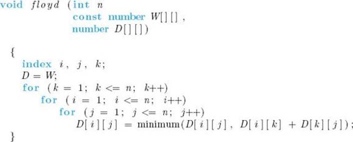
We can perform our calculations using only one array D because the values in the kth row and the kth column are not changed during the kth iteration of the loop. That is, in the kth iteration the algorithm assigns

which clearly equals D [i] [k], and

which clearly equals D [k] [j]. During the kth iteration, D [i] [j] is computed from only its own value and values in the kth row and the kth column. Because these values have maintained their values from the (k − 1)st iteration, they are the values we want. As mentioned before, sometimes after developing a dynamic programming algorithm, it is possible to revise the algorithm to make it more efficient in terms of space.

Next we analyze Floyd’s Algorithm.

Analysis of Algorithm 3.3

Every-Case Time Complexity (Floyd’s Algorithm for Shortest Paths)

Basic operation: The instruction in the for-j loop.

Input size: n, the number of vertices in the graph.

We have a loop within a loop within a loop, with n passes through each loop. So

The following modification to Algorithm 3.3 produces shortest paths.

Algorithm 3.4

Floyd’s Algorithm for Shortest Paths 2

Problem: Same as in Algorithm 3.3, except shortest paths are also created.

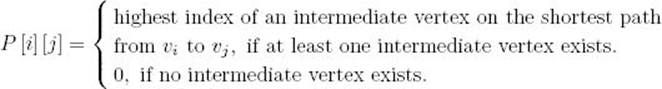
Additional outputs: an array P, which has both its rows and columns indexed from 1 to n, where

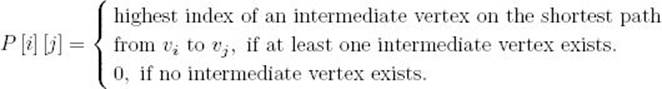
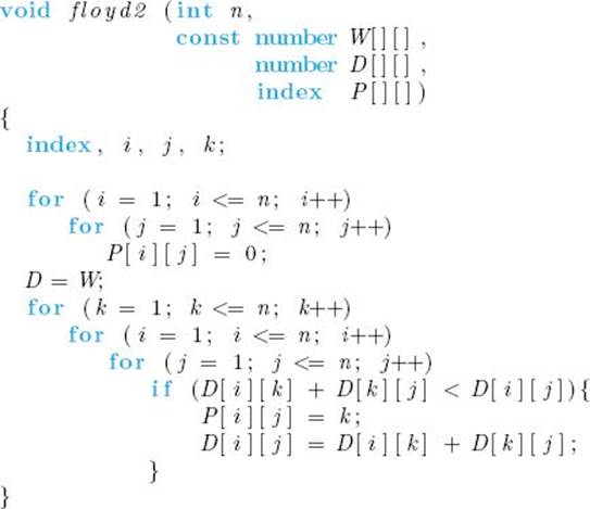
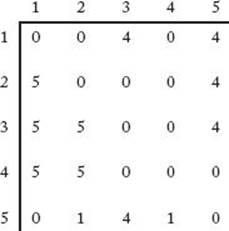
Figure 3.5 shows the array P that is created when the algorithm is applied to the graph in Figure 3.2.

The following algorithm produces a shortest path from vertex v_q to v_r using the array P.

Figure 3.5 The array P produced when Algorithm 3.4 is applied to the graph in Figure 3.2.

Algorithm 3.5

Print Shortest Path

Problem: Print the intermediate vertices on a shortest path from one vertex to another vertex in a weighted graph.

Inputs: the array P produced by Algorithm 3.4, and two indices, q and r, of vertices in the graph that is the input to Algorithm 3.4.

Outputs: the intermediate vertices on a shortest path from v_q to v_r.

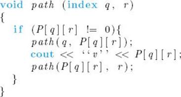
Recall the convention established in Chapter 2 of making only variables, whose values can change in the recursive calls, inputs to recursive routines. Therefore, the array P is not an input to path. If the algorithm were implemented by defining P globally, and we wanted a shortest path from v_q tov_r, the top-level call to path would be as follows:

path (q , r) ;

Given the value of P in Figure 3.5, if the values of q and r were 5 and 3, respectively, the output would be

These are the intermediate vertices on a shortest path from v₅ to v₃.

In the exercises we establish that W(n) ∈ Θ(n) for Algorithm 3.5.

3.3 Dynamic Programming and Optimization Problems

Recall that Algorithm 3.4 not only determines the lengths of the shortest paths but also constructs shortest paths. The construction of the optimal solution is a third step in the development of a dynamic programming algorithm for an optimization problem. This means that the steps in the development of such an algorithm are as follows:

1. Establish a recursive property that gives the optimal solution to an instance of the problem.

2. Compute the value of an optimal solution in a bottom-up fashion.

3. Construct an optimal solution in a bottom-up fashion.

Steps 2 and 3 are ordinarily accomplished at about the same point in the algorithm. Because Algorithm 3.2 is not an optimization problem, there is no third step.

Although it may seem that any optimization problem can be solved using dynamic programming, this is not the case. The principle of optimality must apply in the problem. That principle can be stated as follows:

Definition

The principle of optimality is said to apply in a problem if an optimal solution to an instance of a problem always contains optimal solutions to all substances.

The principle of optimality is difficult to state and can be better understood by looking at an example. In the case of the Shortest Paths problem we showed that if v_k is a vertex on an optimal path from v_i to v_j, then the subpaths from v_i to v_k and from v_k to v_j must also be optimal. Therefore, the optimal solution to the instance contains optimal solutions to all subinstances, and the principle of optimality applies.

If the principle of optimality applies in a given problem, we can develop a recursive property that gives an optimal solution to an instance in terms of optimal solutions to subinstances. The important but subtle reason why we can then use dynamic programming to construct an optimal solution to an instance is that the optimal solutions to the subinstances can be any optimal solutions. For example, in the case of the Shortest Paths problem, if the subpaths are any shortest paths, the combined path will be optimal. We can therefore use the recursive property to construct optimal solutions to increasingly large instances from the bottom up. Each solution along the way will always be optimal.

Although the principle of optimality may appear obvious, in practice it is necessary to show that the principle applies before assuming that an optimal solution can be obtained using dynamic programming. The following example shows that it does not apply in every optimization problem.

Example 3.4

Consider the Longest Paths problem of finding the longest simple paths from each vertex to all other vertices. We restrict the Longest Paths problem to simple paths because with a cycle we can always create an arbitrarily long path by repeatedly passing through the cycle. In Figure 3.6 the optimal (longest) simple path from v₁ to v₄ is [v₁, v₃, v₂, v₄]. However, the subpath [v₁, v₃] is not an optimal (longest) path from v₁ to v₃ because

Figure 3.6 A weighted, directed graph with a cycle.

Therefore, the principle of optimality does not apply. The reason for this is that the optimal paths from v₁ to v₃ and from v₃ to v₄ cannot be strung together to give an optimal path from v₁ to v₄. Doing this would create a cycle rather than an optimal path.

The remainder of this chapter is concerned with optimization problems. When developing the algorithms, we will not explicitly mention the steps outlined earlier. It should be clear that they are being followed.

3.4 Chained Matrix Multiplication

Suppose we want to multiply a 2 × 2 matrix times a 3 × 4 matrix as follows:

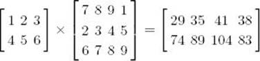
The resultant matrix is a 2 × 4 matrix. If we use the standard method of multiplying matrices (that is, the one obtained from the definition of matrix multiplication), it takes three elementary multiplications to compute each item in the product. For example, the first item in the first column is given by

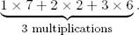
Because there are 2 × 4 = 8 entries in the product, the total number of elementary multiplication is

In general, to multiply an i × j matrix times a j × k matrix using the standard method, it is necessary to do

Consider the multiplication of the following four matrices:

The dimension of each matrix appears under the matrix. Matrix multiplication is an associative operation, meaning that the order in which we multiply does not matter. For example, A(B (CD)) and (AB) (CD) both give the same answer. There are five different orders in which we can multiply four matrices, each possibly resulting in a different number of elementary multiplications. In the case of the previous matrices, we have the following number of elementary multiplications for each order.

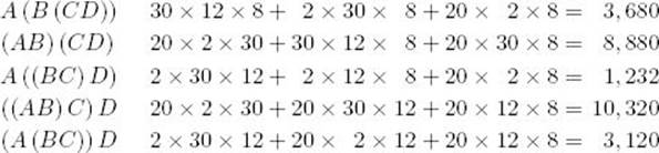
The third order is the optimal order for multiplying the four matrices.

Our goal is to develop an algorithm that determines the optimal order for multiplying n matrices. The optimal order depends only on the dimensions of the matrices. Therefore, besides n, these dimensions would be the only input to the algorithm. The brute-force algorithm is to consider all possible orders and take the minimum, as we just did. We will show that this algorithm is at least exponential-time. To this end, let t_n be the number of different orders in which we can multiply n matrices: A₁, A₂, … , A_n. A subset of all the orders is the set of orders for which A₁ is the last matrix multiplied. As illustrated below, the number of different orders in this subset is t_n−1, because it is the number of different orders with which we can multiply A₂ through A_n:

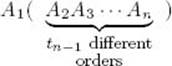
A second subset of all the orders is the set of orders for which A_n is the last matrix multiplied. Clearly, the number of different orders in this subset is also t_n−1. Therefore,

Because there is only one way to multiply two matrices, t₂ = 1. Using the techniques in Appendix B, we can solve this recurrence to show that

It is not hard to see that the principle of optimality applies in this problem. That is, the optimal order for multiplying n matrices includes the optimal order for multiplying any subset of the n matrices. For example, if the optimal order for multiplying six particular matrices is

then

must be the optimal order for multiplying matrices A₂ through A₄. This means we can use dynamic programming to construct a solution.

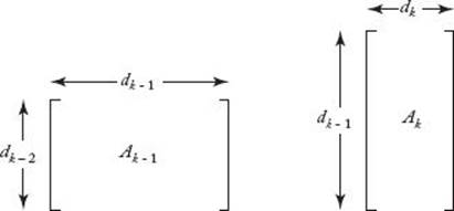
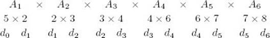
Because we are multiplying the (k − 1)st matrix, A_k−1, times the kth matrix, A_k, the number of columns in A_k−1 must equal the number of rows in A_k. For example, in the product discussed earlier, the first matrix has three columns and the second has three rows. If we let d₀ be the number of rows inA₁ and d_k be the number of columns in A_k for 1 ≤ k ≤ n, the dimension of A_k is d_k−1 × d_k. This is illustrated in Figure 3.7.

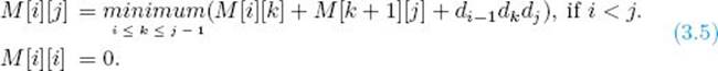
As in the previous section, we will use a sequence of arrays to construct our solution. For 1 ≤ i ≤ j ≤ n, let

M [i] [j] = minimum number of multiplications needed to multiply A_i through A_j, if i < j.

M [i] [i] = 0.

Before discussing how we will use these arrays, let’s illustrate the meanings of the items in them.

Figure 3.7 The number of columns in A_k−1 is the same as the number of rows

Example 3.5

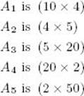
Suppose we have the following six matrices:

To multiply A₄, A₅, and A₆, we have the following two orders and numbers of elementary multiplications:

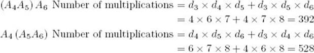
Therefore,

The optimal order for multiplying six matrices must have one of these factorizations:

1. A₁ (A₂A₃A₄A₅A₆)

2. (A₁A₂) (A₃A₄A₅A₆)

3. (A₁A₂A₃) (A₄A₅A₆)

4. (A₁A₂A₃A₄) (A₅A₆)

5 (A₁A₂A₃A₄A₅) A₆

where inside each parentheses the products are obtained according to the optimal order for the matrices inside the parentheses. Of these factorizations, the one that yields the minimum number of multiplications must be the optimal one. The number of multiplications for the kth factorization is the minimum number needed to obtain each factor plus the number needed to multiply the two factors. This means that it equals

We have established that

There is nothing in the preceding argument that restricts the first matrix to being A₁ or the last matrix to being A₆. For example, we could have obtained a similar result for multiplying A₂ through A₆. Therefore, we can generalize this result to obtain the following recursive property when multiplyingn matrices. For 1 ≤ i ≤ j ≤ n

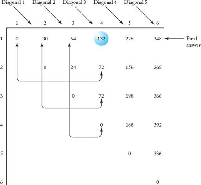
A divide-and-conquer algorithm based on this property is exponential-time. We develop a more efficient algorithm using dynamic programming to compute the values of M [i] [j] in steps. A grid similar to Pascal’s triangle is used (see Section 3.1). The calculations, which are a little more complex than those in Section 3.1, are based on the following property of Equality 3.5: M [i] [j] is calculated from all entries on the same row as M [i] [j] but to the left of it, along with all entries in the same column as M [i] [j] but beneath it. Using this property, we can compute the entries in M as follows: First we set all those entries in the main diagonal to 0; next we compute all those entries in the diagonal just above it, which we call diagonal 1; next we compute all those entries in diagonal 2; and so on. We continue in this manner until we compute the only entry in diagonal 5, which is our final answer, M [1] [6]. This procedure is illustrated in Figure 3.8 for the matrices in Example 3.5. The following example shows the calculations.

Example 3.6

Suppose we have the six matrices in Example 3.5. The steps in the dynamic programming algorithm follow. The results appear in Figure 3.8.

Compute diagonal 0:

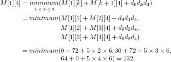
Compute diagonal 1:

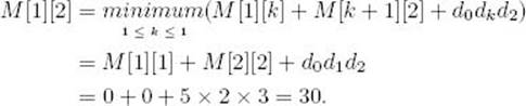
Figure 3.8 The array M developed in Example 3.5. M [1] [4], which is circled, is computed from the pairs of entries indicated

The values of M [2] [3], M [3] [4], M [4] [5], and M [5] [6] are computed in the same way. They appear in Figure 3.8.

Compute diagonal 2:

The values of M [2] [4], M [3] [5], and M [4] [6] are computed in the same way and are shown in Figure 3.8.

Compute diagonal 3:

The values of M [2] [5] and M [3] [6] are computed in the same manner and are shown in Figure 3.8.

Compute diagonal 4:

The entries in diagonal 4 are computed in the same manner and are shown in Figure 3.8.

Compute diagonal 5:

Finally, the entry in diagonal 5 is computed in the same manner. This entry is the solution to our instance; it is the minimum number of elementary multiplications, and its value is given by

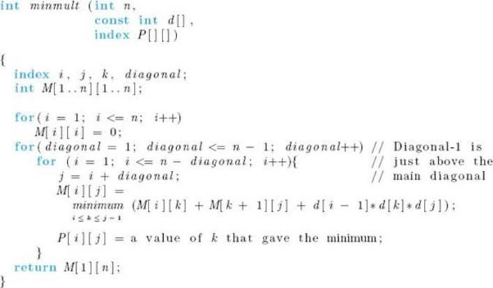
The algorithm that follows implements this method. The dimensions of the n matrices—namely, the values of d₀ through d_n—are the only inputs to the algorithm. Matrices themselves are not inputs because the values in the matrices are irrelevant to the problem. The array P produced by the algorithm can be used to print the optimal order. We discuss this after analyzing Algorithm 3.6.

Algorithm 3.6

Minimum Multiplications

Problem: Determining the minimum number of elementary multiplications needed to multiply n matrices and an order that produces that minimum number.

Inputs: the number of matrices n, and an array of integers d, indexed from 0 to n, where d [i − 1] × d [i] is the dimension of the ith matrix.

Outputs: minmult, the minimum number of elementary multiplications needed to multiply the n matrices; a two-dimensional array P from which the optimal order can be obtained. P has its rows indexed from 1 to n − 1 and its columns indexed from 1 to n. P [i] [j] is the point where matrices ithrough j are split in an optimal order for multiplying the matrices.

Next we analyze Algorithm 3.6.

Analysis of Algorithm 3.6

Every-Case Time Complexity (Minimum Multiplications)

Basic operation: We can consider the instructions executed for each value of k to be the basic operation. Included is a comparison to test for the minimum.

Input size: n, the number of matrices to be multiplied.

We have a loop within a loop within a loop. Because j = i + diagonal, for given values of diagonal and i, the number of passes through the k loop is

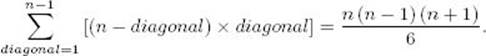
For a given value of diagonal, the number of passes through the for-i loop is n − diagonal. Because diagonal goes from 1 to n − 1, the total number of times the basic operation is done equals

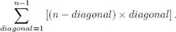
In the exercises we establish that this expression equals

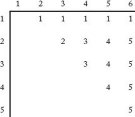
Next we show how an optimal order can be obtained from the array P. The values of that array, when the algorithm is applied to the dimensions in Example 3.5, are shown in Figure 3.9. The fact that, for example, P [2] [5] = 4 means that the optimal order for multiplying matrices A₂ through A₅has the factorization

where inside the parentheses the matrices are multiplied according to the optimal order. That is, P [2] [5], which is 4, is the point where the matrices should be split to obtain the factors. We can produce an optimal order by visiting P [1] [n] first to determine the top-level factorization. Because n = 6 and P [1, 6] = 1, the top-level factorization in the optimal order is

Next we determine the factorization in the optimal order for multiplying A₂ through A₆ by visiting P [2] [6]. Because the value of P [2] [6] is 5, that factorization is

We now know that the factorization in the optimal order is

where the factorization for multiplying A₂ through A₅ must still be determined. Next we look up P [2] [5] and continue in this manner until all the factorizations are determined. The answer is

Figure 3.9 The array P produced when Algorithm 3.6 is applied to the dimensions in Example 3.5.

The following algorithm implements the method just described.

Algorithm 3.7

Print Optimal Order

Problem: Print the optimal order for multiplying n matrices.

Inputs: Positive integer n, and the array P produced by Algorithm 3.6. P [i] [j] is the point where matrices i through j are split in an optimal order for multiplying those matrices.

Outputs: the optimal order for multiplying the matrices.

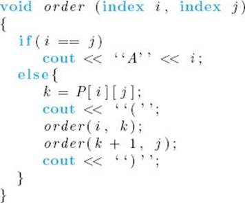
Following our usual convention for recursive routines, P and n are not inputs to order, but are inputs to the algorithm. If the algorithm were implemented by defining P and n globally, the top-level call to order would be as follows:

order (1 , n) ;

When the dimensions are those in Example 3.5, the algorithm prints the following:

There are parentheses around the entire expression because the algorithm puts parentheses around every compound term. In the exercises we establish for Algorithm 3.7 that

Our Θ(n³) algorithm for chained matrix multiplication is from Godbole (1973). Yao (1982) developed methods for speeding up certain dynamic programming solutions. Using those methods, it is possible to create a Θ(n²) algorithm for chained matrix multiplication. Hu and Shing (1982, 1984) describe a Θ(n lg n) algorithm for chained matrix multiplication.

3.5 Optimal Binary Search Trees

Next we obtain an algorithm for determining the optimal way of organizing a set of items in a binary search tree. Before discussing what kind of organization is considered optimal, let’s review such trees. For any node in a binary tree, the subtree whose root is the left child of the node is called theleft subtree of the node. The left subtree of the root of the tree is called the left subtree of the tree. The right subtree is defined analogously.

Definition

A binary search tree is a binary tree of items (ordinarily called keys), that come from an ordered set, such that

1. Each node contains one key.

2. The keys in the left subtree of a given node are less than or equal to the key in that node.

3. The keys in the right subtree of a given node are greater than or equal to the key in that node.

Figure 3.10 shows two binary search trees, each with the same keys. In the tree on the left, look at the right subtree of the node containing “Ralph.” That subtree contains “Tom,” “Ursula,” and “Wally,” and these names are all greater than “Ralph” according to an alphabetic ordering. Although, in general, a key can occur more than once in a binary search tree, for simplicity we assume that the keys are distinct.

Figure 3.10 Two binary search trees.

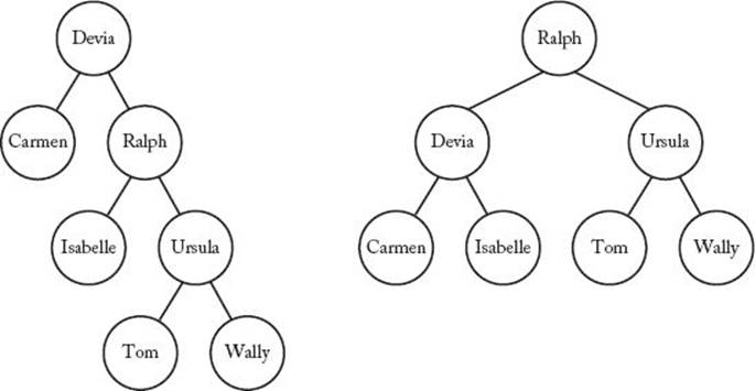
The depth of a node in a tree is the number of edges in the unique path from the root to the node. This is also called the level of the node in the tree. Usually we say that a node has a depth and that the node is at a level. For example, in the tree on the left in Figure 3.10, the node containing “Ursula” has a depth of 2. Alternatively, we could say that the node is at level 2. The root has a depth of 0 and is at level 0. The depth of a tree is the maximum depth of all nodes in the tree. The tree on the left in Figure 3.10 has a depth of 3, whereas the tree on the right has a depth of 2. A binary tree is called balanced if the depth of the two subtrees of every node never differ by more than 1. The tree on the left in Figure 3.10 is not balanced because the left subtree of the root has a depth of 0, and the right subtree has a depth of 2. The tree on the right in Figure 3.10 is balanced.

Ordinarily, a binary search tree contains records that are retrieved according to the values of the keys. Our goal is to organize the keys in a binary search tree so that the average time it takes to locate a key is minimized. (See Section A.8.2 for a discussion of the average.) A tree that is organized in this fashion is called optimal. It is not hard to see that, if all keys have the same probability of being the search key, the tree on the right in Figure 3.10 is optimal. We are concerned with the case where the keys do not have the same probability. An example of this case would be a search of one of the trees in Figure 3.10 for a name picked at random from people in the United States. Because “Tom” is a more common name than “Ursula,” we would assign a greater probability to “Tom.” (See Section A.8.1 in Appendix A for a discussion of randomness.)

We will discuss the case in which it is known that the search key is in the tree. A generalization to the case where it may not be in the tree is investigated in the exercises. To minimize the average search time, we need to know the time complexity of locating a key. Therefore, before proceeding, let’s write and analyze an algorithm that searches for a key in a binary search tree. The algorithm uses the following data types:

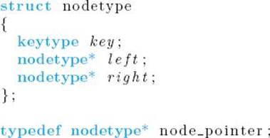
This declaration means that a node pointer variable is a pointer to a nodetype record. That is, its value is the memory address of such a record.

Algorithm 3.8

Search Binary Tree

Problem: Determine the node containing a key in a binary search tree. It is assumed that the key is in the tree.

Inputs: a pointer tree to a binary search tree and a key keyin.

Outputs: a pointer p to the node containing the key.

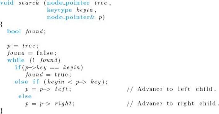
The number of comparisons done by procedure search to locate a key is called the search time. Our goal is to determine a tree for which the average search time is minimal. As discussed in Section 1.2, we assume that comparisons are implemented efficiently. With this assumption, only one comparison is done in each iteration of the while loop in the previous algorithm. Therefore, the search time for a given key is

where depth (key) is the depth of the node containing the key. For example, because the depth of the node containing “Ursula” is 2 in the left tree in Figure 3.10, the search time for “Ursula” is

Let Key₁, Key₂, … , Key_n be the n keys in order, and let p_i be the probability that Key_i is the search key. If c_i is the number of comparisons needed to find Key_i in a given tree, the average search time for that tree is

This is the value we want to minimize.

Example 3.7

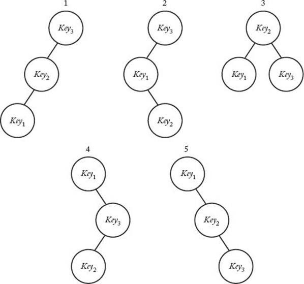
Figure 3.11 shows the five different trees when n = 3. The actual values of the keys are not important. The only requirement is that they be ordered. If

the average search times for the trees in Figure 3.11 are:

1. 3 (0.7) + 2 (0.2) + 1 (0.1) = 2.6

2. 2 (0.7) + 3 (0.2) + 1 (0.1) = 2.1

3. 2 (0.7) + 1 (0.2) + 2 (0.1) = 1.8

4. 1 (0.7) + 3 (0.2) + 2 (0.1) = 1.5

5. 1 (0.7) + 2 (0.2) + 3 (0.1) = 1.4

The fifth tree is optimal.

Figure 3.11 The possible binary search trees when there are three keys.

In general, we cannot find an optimal binary search tree by considering all binary search trees because the number of such trees is at least exponential in n. We prove this by showing that if we just consider all binary search trees with a depth of n − 1, we have an exponential number of trees. In a binary search tree with a depth of n − 1, the single node at each of the n − 1 levels beyond the root can be either to the left or to the right of its parent, which means there are two possibilities at each of those levels. This means that the number of different binary search trees with a depth of n − 1 is 2ⁿ⁻¹.

Dynamic programming will be used to develop a more efficient algorithm. To that end, suppose that keys Key_i through Key_j are arranged in a tree that minimizes

where c_m is the number of comparisons needed to locate Key_m in the tree. We will call such a tree optimal for those keys and denote the optimal value by A [i] [j]. Because it takes one comparison to locate a key in a tree containing one key, A [i] [i] = p_i.

Example 3.8

Suppose we have three keys and the probabilities in Example 3.7. That is,

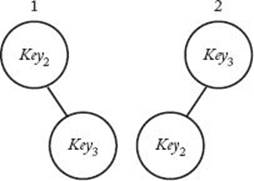
To determine A [2] [3] we must consider the two trees in Figure 3.12. For those two trees we have the following:

1. 1 (p₂) + 2 (p₃) = 1 (0.2) + 2 (0.1) = 0.4

2. 2 (p₂) + 1 (p₃) = 2 (0.2) + 1 (0.1) = 0.5

The first tree is optimal, and

Figure 3.12 The binary search trees composed of Key₂ and Key₃.

Notice that the optimal tree obtained in Example 3.8 is the right subtree of the root of the optimal tree obtained in Example 3.7. Even if this tree was not the exact same one as that right subtree, the average time spent searching in it would have to be the same. Otherwise, we could substitute it for that subtree, resulting in a tree with a smaller average search time. In general, any subtree of an optimal tree must be optimal for the keys in that subtree. Therefore, the principle of optimality applies.

Figure 3.13 Optimal binary search tree given that Key_k is at the root.

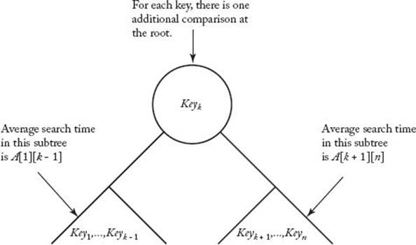
Next, let tree 1 be an optimal tree given the restriction that Key₁ is at the root, tree 2 be an optimal tree given the restriction that Key₂ is at the root, … , tree n be an optimal tree given the restriction that Key_n is at the root. For 1 ≤ k ≤ n, the subtrees of tree k must be optimal, and therefore the average search times in these subtrees are as depicted in Figure 3.13. This figure also shows that for each m ≠ k it takes exactly one more comparison (the one at the root) to location Key_m in tree k than it does to locate that key in the subtree that contains it. This one comparison adds 1 × p_m to the average search time for Key_m in tree k. We’ve established that the average search time for tree k is given by

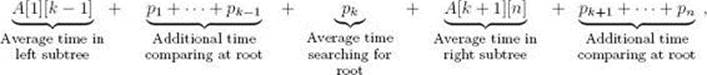
which equals

Because one of the k trees must be optimal, the average search time for the optimal tree is given by

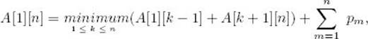
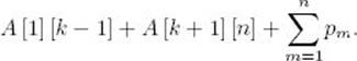
where A [1] [0] and A [n + 1] [n] are defined to be 0. Although the sum of the probabilities in this last expression is clearly 1, we have written it as a sum because we now wish to generalize the result. To that end, there is nothing in the previous discussion that requires that the keys be Key₁ throughKey_n. That is, in general, the discussion pertains to Key_i through Key_j, where i < j. We have therefore derived the following:

Using Equality 3.6, we can write an algorithm that determines an optimal binary search tree. Because A [i] [j] is computed from entries in the ith row but to the left of A [i] [j] and from entries in the jth column but beneath A [i] [j], we proceed by computing in sequence the values on each diagonal (as was done in Algorithm 3.6). Because the steps in the algorithm are so similar to those in Algorithm 3.6, we do not include an example illustrating these steps. Rather, we simply give the algorithm followed by a comprehensive example showing the results of applying the algorithm. The array R produced by the algorithm contains the indices of the keys chosen for the root at each step. For example, R [1] [2] is the index of the key in the root of an optimal tree containing the first two keys, and R [2] [4] is the index of the key in the root of an optimal tree containing the second, third, and fourth keys. After analyzing the algorithm, we will discuss how to build an optimal tree from R.

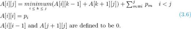
Algorithm 3.9

Optimal Binary Search Tree

Problem: Determine an optimal binary search tree for a set of keys, each with a given probability of being the search key.

Inputs: n, the number of keys, and an array of real numbers p indexed from 1 to n, where p [i] is the probability of searching for the ith key.

Outputs: A variable minavg, whose value is the average search time for an optimal binary search tree; and a two-dimensional array R from which an optimal tree can be constructed. R has its rows indexed from 1 to n+1 and its columns indexed from 0 to n. R [i] [j] is the index of the key in the root of an optimal tree containing the ith through the jth keys.

Analysis of Algorithm 3.9

Every-Case Time Complexity (Optimal Binary Search Tree)

Basic operation: The instructions executed for each value of k. They include a comparison to test for the minimum. The value of does not need to be computed from scratch each time. In the exercises you will find an efficient way to compute these sums.

Input size: n, the number of keys.

The control of this algorithm is almost identical to that in Algorithm 3.6. The only difference is that, for given values of diagonal and i, the basic operation is done diagonal+1 times. An analysis like the one of Algorithm 3.6 establishes that

The following algorithm constructs a binary tree from the array R. Recall that R contains the indices of the keys chosen for the root at each step.

Algorithm 3.10

Build Optimal Binary Search Tree

Problem: Build an optimal binary search tree.

Inputs: n, the number of keys, an array Key containing the n keys in order, and the array R produced by Algorithm 3.9. R [i] [j] is the index of the key in the root of an optimal tree containing the ith through the jth keys.

Outputs: a pointer tree to an optimal binary search tree containing the n keys.

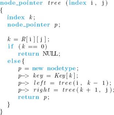
The instruction p = new nodetype gets a new node and puts its address in p. Following our convention for recursive algorithms, the parameters n, Key, and R are not inputs to function tree. If the algorithm were implemented by defining n, Key, and R globally, a pointer root to the root of an optimal binary search tree is obtained by calling tree as follows:

root = tree (1, n);

We did not illustrate the steps in Algorithm 3.9 because it is similar to Algorithm 3.6 (Minimum Multiplications). Likewise, we will not illustrate the steps in Algorithm 3.10 because this algorithm is similar to Algorithm 3.7 (Print Optimal Order). Rather, we provide one comprehensive example showing the results of applying both Algorithms 3.9 and 3.10.

Example 3.9

Supposed we have the following values of the array Key:

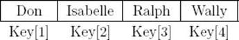
and

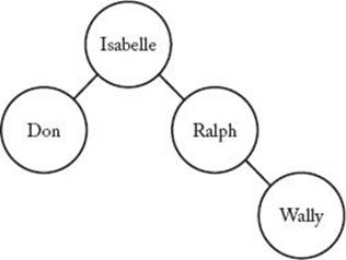
The arrays A and R produced by Algorithm 3.9 are shown in Figure 3.14, and the tree created by Algorithm 3.10 is shown in Figure 3.15. The minimal average search time is 7/4.

Figure 3.14 The arrays A and R, produced when Algorithm 3.9 is applied to the instance in Example 3.9.

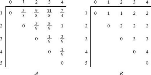
Notice that R [1] [2] could be 1 or 2. The reason is that either of these indices could be the index of the root in an optimal tree containing only the first two keys. Therefore, both of these indices give the minimum value of A [1] [2] in Algorithm 3.9, which means that either could be chosen for R[1] [2].

Figure 3.15 The tree produced when Algorithms 3.9 and 3.10 are applied to the instance in Example 3.9.

The previous algorithm for determining an optimal binary search tree is from Gilbert and Moore (1959). A Θ(n²) algorithm can be obtained using the dynamic programming speed-up method in Yao (1982).

3.6 The Traveling Salesperson Problem

Suppose a salesperson is planning a sales trip that includes 20 cities. Each city is connected to some of the other cities by a road. To minimize travel time, we want to determine a shortest route that starts at the salesperson’s home city, visits each of the cities once, and ends up at the home city. This problem of determining a shortest route is called the Traveling Salesperson problem.

An instance of this problem can be represented by a weighted graph, in which each vertex represents a city. As in Section 3.2, we generalize the problem to include the case in which the weight (distance) going in one direction can be different from the weight going in another direction. Again we assume that the weights are nonnegative numbers. Figures 3.2 and 3.16 show such weighted graphs. A tour (also called a Hamiltonian circuit) in a directed graph is a path from a vertex to itself that passes through each of the other vertices exactly once. An optimal tour in a weighted, directed graph is such a path of minimum length. The Traveling Salesperson problem is to find an optimal tour in a weighted, directed graph when at least one tour exists. Because the starting vertex is irrelevant to the length of an optimal tour, we will consider v₁ to be the starting vertex. The following are the three tours and lengths for the graph in Figure 3.16:

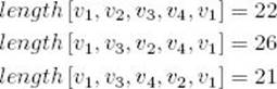
The last tour is optimal. We solved this instance by simply considering all possible tours. In general, there can be an edge from every vertex to every other vertex. If we consider all possible tours, the second vertex on the tour can be any of n−1 vertices, the third vertex on the tour can be any of n − 2 vertices, … , the nth vertex on the tour can be only one vertex. Therefore, the total number of tours is

Figure 3.16 The optimal tour is [v₁, v₃, v₄, v₂, v₁].

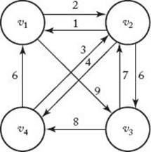
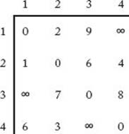
Figure 3.17 The adjacency matrix representation W of the graph in Figure 3.16.

which is worse than exponential.

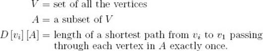
Can dynamic programming be applied to this problem? Notice that if v_k is the first vertex after v₁ on an optimal tour, the subpath of that tour from v_k to v₁ must be a shortest path from v_k to v₁ that passes through each of the other vertices exactly once. This means that the principle of optimality applies, and we can use dynamic programming. To that end, we represent the graph by an adjacency matrix W, as was done in Section 3.2. Figure 3.17 shows the adjacency matrix representation of the graph in Figure 3.16. Let

Example 3.10

For the graph in Figure 3.16,

Notice that {v₁, v₂, v₃, v₄} uses curly braces to represent a set, whereas [v₁, v₂, v₃, v₄] uses square brackets to represent a path. If A = {v₃}, then

If A = {v₃, v₄}, then

Because V − {v₁, v_j} contains all the vertices except v₁ and v_j and the principle of optimality applies, we have

and, in general for i ≠ 1 and v_i not in A,

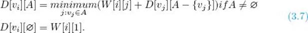
We can create a dynamic programming algorithm for the Traveling Salesperson problem using Equality 3.7. But first, let’s illustrate how the algorithm would proceed.

Example 3.11

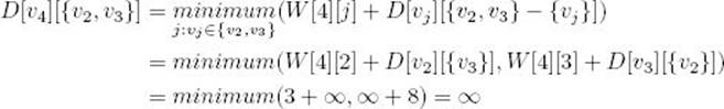
Determine an optimal tour for the graph represented in Figure 3.17. First consider the empty set:

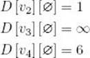
Next consider all sets containing one element:

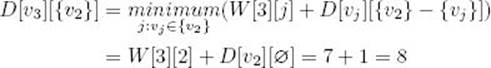
Similarly,

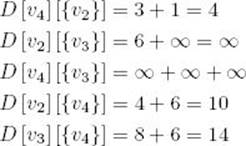
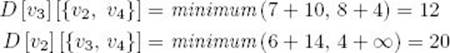
Next consider all sets containing two elements:

Similarly,

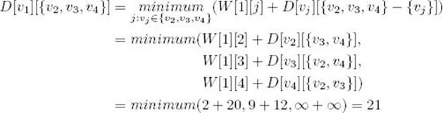
Finally, compute the length of an optimal tour:

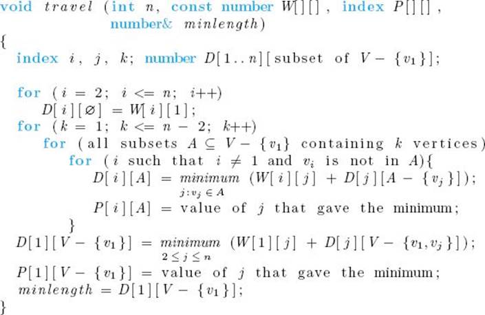
The dynamic programming algorithm for the Traveling Salesperson problem follows.

Algorithm 3.11

The Dynamic Programming Algorithm for the Traveling Salesperson Problem

Problem: Determine an optimal tour in a weighted, directed graph. The weights are nonnegative numbers.

Inputs: a weighted, directed graph, and n, the number of vertices in the graph. The graph is represented by a two-dimensional array W, which has both its rows and columns indexed from 1 to n, where W [i] [j] is the weight on the edge from ith vertex to the jth vertex.

Outputs: a variable minlength, whose value is the length of an optimal tour, and a two-dimensional array P from which an optimal tour can be constructed. P has its rows indexed from 1 to n and its columns indexed by all subsets of V − {v₁}. P [i] [A] is the index of the first vertex after v_i on a shortest path from v_i to v₁ that passes through all vertices in A exactly once.

Before showing how an optimal tour can be obtained from the array P, we analyze the algorithm. First we need a theorem:

Theorem 3.1

For all n ≥ 1

Proof: It is left as an exercise to show that

Therefore,

The last equality is obtained by applying the result found in Example A.10 in Appendix A.

The analysis of Algorithm 3.11 follows.

Analysis of Algorithm 3.11

Every-Case Time and Space Complexity (The Dynamic Programming Algorithm for the Traveling Salesperson Problem)

Basic operation: The time in both the first and last loops is insignificant compared to the time in the middle loop because the middle loop contains various levels of nesting. Therefore, we will consider the instructions executed for each value of v_j to be the basic operation. They include an addition instruction.

Input size: n, the number of vertices in the graph.

For each set A containing k vertices, we must consider n − 1 − k vertices, and for each of these vertices, the basic operation is done k times. Because the number of subsets A of V −{v₁} containing k vertices is equal to the total number of times the basic operation is done is given by

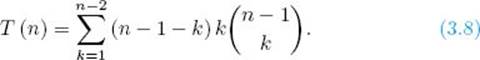
It is not hard to show that

Substituting this equality into Equality 3.8, we have

Finally, applying Theorem 3.1, we have

Because the memory used in this algorithm is also large, we will analyze the memory complexity, which we call M (n). The memory used to store the arrays D [v_i] [A] and P [v_i] [A] is clearly the dominant amount of memory. So we will determine how large these arrays must be. Because V − {v₁} contains n − 1 vertices, we can apply the result in Example A.10 in Appendix A to conclude that it has 2ⁿ⁻¹ subsets A. The first index of the arrays D and P ranges in value between 1 and n. Therefore,

At this point you may be wondering what we have gained, because our new algorithm is still Θ(n²2ⁿ) The following example shows that even an algorithm with this time complexity can sometimes be useful.

Example 3.12

Ralph and Nancy are both competing for the same sales position. The boss tells them on Friday that, starting on Monday, whoever can cover the entire 20-city territory faster will get the position. The territory includes the home office, and they must return to the home office when they are done. There is a road from every city to every other city. Ralph figures he has the whole weekend to determine his route; so he simply runs the brute-force algorithm that considers all (20 − 1)! tours on his computer. Nancy recalls the dynamic programming algorithm from her algorithms course. Figuring she should take every advantage she can, she runs that algorithm on her computer. Assuming that the time to process the basic instruction in Nancy’s algorithm is 1 microsecond, and that it takes 1 microsecond for Ralph’s algorithm to compute the length of each tour, the time taken by each algorithm is given approximately by the following:

Dynamic programming algorithm: (20 − 1) (20 − 2) 2²⁰⁻³ µs = 45 seconds.

We see that even a Θ(n²2ⁿ)algorithm can be useful when the alternative is a factorial-time algorithm. The memory used by the dynamic programming algorithm in this example is

Although this is quite large, it is feasible by today’s standards.

Using the Θ(n²2ⁿ) algorithm to find the optimal tour is practical only because n is small. If, for example, there were 60 cities, that algorithm, too, would take many years.

Let’s discuss how to retrieve an optimal tour from the array P. We don’t give the algorithm; rather, we simply illustrate how it would proceed. The members of the array P needed to determine an optimal tour for the graph represented in Figure 3.16 are:

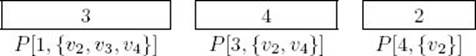
We obtain an optimal tour as follows:

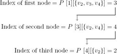
The optimal tour is, therefore,

No one has ever found an algorithm for the Traveling Salesperson problem whose worst-case time complexity is better than exponential. Yet no one has ever proved that such an algorithm is not possible. This problem is one of a large class of closely related problems that share this property and are the focus of Chapter 9.

3.7 Sequence Alignment

We show an application of a dynamic program to molecular genetics, namely a homologous DNA sequence alignment. First, we briefly review some concepts in genetics.

A chromosome is a long, threadlike macromolecule consisting of the compound deoxyribonucleic acid (DNA). Chromosomes are the carriers of biologically expressed hereditary characteristics. DNA is composed of two complementary strands, each strand consisting of a sequence of nucleotides. A nucleotide contains a pentose sugar (deoxyribose), a phosphate group, and a purine or pyrimidine base. The purines, adenine (A) and guanine (G), are similar in structure, as are the pyrimidines, cytosine (C) and thymine (T). The strands are joined together by hydrogen bonds between pairs of nucleotides. Adenine always pairs with thymine and guanine always pairs with cytosine. Each pair of these is called a canonical base pair (bp), and A, G, C, and T are called bases.

A section of DNA is depicted in Figure 3.18. The strands actually twist around each other to form a right-handed double helix. However, for our purposes, we need only consider them as character strings as shown. It is believed that a chromosome is just one long DNA molecule.

A DNA sequence is a section of DNA, and a site is the location of each base pair in the sequence. A DNA sequence can undergo a substitution mutation that means one nucleotide is substituted by another, an insertion mutation that means a base pair is inserted in the sequence, and adeletion mutation that means a base pair is deleted from the sequence.

Consider the same DNA sequence in every individual in a particular population (species). In each generation, each site in the sequence has a probability of undergoing a mutation in each gamete that produces an individual for the next generation. A possible result is substitution at a given site of one base by another base in the entire population (or much of it). Another possible result would be that a speciation event eventually occurs, which means that the members of the species separate into two different species. In this case, the total substitutions that eventually occur in one of the species can be quite different from those that occur in the other species. This means that the sequences in individuals, taken from each of the two species, may be quite different. We say that the sequences have diverged. The corresponding sequences from the two species are called homologous sequences. In a phylogenetic tree inference, we are interested in comparing homologous sequences from different species and estimating their distance in an evolutionary sense.

Figure 3.18 A section of DNA.

When we compare homologous sequences from two individuals in two different species, we must first align the sequences because one or both of the sequences may have undergone insertion and/or deletion mutations since they diverged. For example, an alignment of the first introns of the human and owl monkey insulin genes results in a 196-nucleotide sequence in which 163 of the sites do not have a gap in either sequence.

Example 3.13

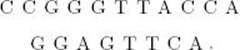
Suppose we have the following homologous sequences:

We could align them in many ways. The following shows two possible alignments:

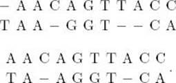
When we include a dash (−) in an alignment, this is called inserting a gap. It indicates that either the sequence with the gap has undergone a deletion or the other sequence has undergone an insertion.

Which alignment in the previous example is better? Both have five matching base pairs. The top alignment has two mismatched base pairs, but at the expense of inserting four gaps. On the other hand, the bottom alignment has three mismatched base pairs but at the expense of inserting only two gaps. In general, it is not possible to say which alignment is better without first specifying the penalty for a mismatch and the penalty for a gap. For example, suppose we say a gap has a penalty of 1 and a mismatch has a penalty of 3. We call the sum of all the penalties in an alignment the cost of the alignment. Given these penalty assignments, the top alignment in Example 3.13 has a cost of 10, whereas the bottom one has a cost of 11. So, the top one is better. On the other hand, if we say a gap has a penalty of 2 and a mismatch has a penalty of 1, it is not hard to see that the bottom alignment has a smaller cost and is therefore better.

Once we do specify the penalties for gaps and mismatches, it is possible to determine the optimal alignment. However, doing this by checking all possible alignments is an intractable task. Next, we develop an efficient dynamic programming algorithm for the sequence alignment problem.

For the sake of concreteness, we assume the following:

The penalty for a mismatch is 1.

The penalty for a gap is 2.

First, we represent the two sequences in arrays as follows:

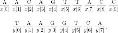
Let opt(i, j) be the cost of the optimal alignment of the subsequences x[i..9] and y[j..7]. Then opt(0, 0) is the cost of the optimal alignment of x[0..9] and y[0..7], which is the alignment we want to perform. This optimal alignment must start with one of the following.

1. x[0] is aligned with y[0]. If x[0] = y[0] there is no penalty at the first alignment site, whereas if x[0] ≠ y[0] there is a penalty of 1.

2. x[0] is aligned with a gap and there is a penalty of 2 at the first alignment site.

3. y[0] is aligned with a gap and there is a penalty of 2 at the first alignment site.

Suppose the optimal alignment A_opt of x[0..9] and y[0..7] has x[0] aligned with y[0]. Then this alignment contains within it an alignment B of x[1..9] and y[1..7]. Suppose this is not the optimal alignment of these two subsequences. Then there is some other alignment C that has a smaller cost. Thus, alignment C, along with aligning x[0] with y[0], will yield an alignment of x[0..9] and y[0..7] and has a smaller cost than A_opt. So, alignment B must be the optimal alignment of x[1..9] and y[1..7]. Similarly, if the optimal alignment of x[0..9] and y[0..7] has x[0] aligned with a gap, then that alignment contains within it the optimal alignment of x[1..9] and y[0..7], and if the optimal alignment of x[0..9] and y[0..7] has y[0] aligned with a gap, then that alignment contains within it the optimal alignment of x[0..9] and y[1..7].

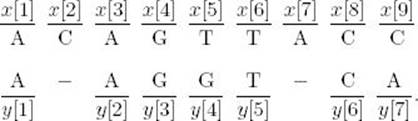
Example 3.14

Suppose the following is an optimal alignment of x[0..9] and y[0..7]:

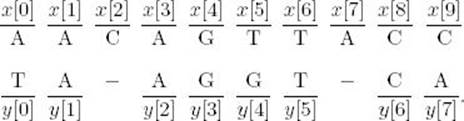
Then the following must be an optimal alignment of x[1..9] and y[1..7]:

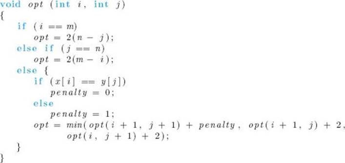
If we let penalty = 0 if x[0] = y[0] and 1 otherwise, we have established the following recursive property:

opt(0, 0) = min(opt(1, 1) + penalty, opt(1, 0) + 2, opt(0, 1) + 2).

Although we illustrated this recursive property starting at the 0th position in both sequences, it clearly holds if we start at arbitrary positions. So, in general,

To complete the development of a recursive algorithm, we need terminal conditions. Let m be the length of sequence x and n be the length of sequence y. If we have passed the end of sequence x (i = m), and we are at the jth position in sequence y, where j < n, then we must insert n − j gaps. So, one terminal condition is

Similarly, if we have passed the end of sequence y (j = n), and we are at the ith position in sequence x, where i < m, then we must insert m − i gaps. So, another terminal condition is

We now have the following divide-and-conquer algorithm:

Algorithm 3.12

Sequence Alignment Using Divide-and-Conquer

Problem: Determine an optimal alignment of two homologous DNA sequences.

Inputs: A DNA sequence x of length m and a DNA sequence y of length n. The sequences are represented in arrays.

Outputs: The cost of an optimal alignment of the two sequences.

The top-level call to the algorithm is

Note that this algorithm only gives the cost of an optimal alignment; it does not produce one. It could be modified to also produce one. However, we will not pursue that here because the algorithm is very inefficient and is therefore not the one we would actually use. It is left as an exercise to show that it has exponential-time complexity.

The problem is that many subinstances are evaluated more than once. For example, to evaluate opt(0, 0) at the top level, we need to evaluate opt(1, 1), opt(1, 0), and opt(0, 1). To evaluate opt(1, 0) in the first recursive call, we need to evaluate opt(2, 1), opt(2, 0), and opt(1, 1). The two evaluations of opt(1, 1) will unnecessarily be done independently.

Figure 3.19 The array used to find the optimal alignment.

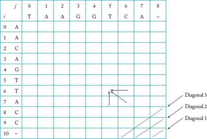
To solve the problem using dynamic programming, we create an m + 1 by n + 1 array, as shown in Figure 3.19 for the current instance. Note that we include one extra character in each sequence which is a gap. The purpose of this is to give our upward iteration scheme a starting point. We want to compute and store opt(i, j) in the ijth slot of this array. Recall that we have the following equalities:

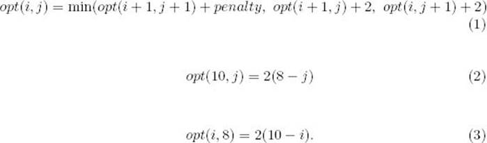
Note that we have put the current instance’s values of m and n in the formulas. If we are in the bottom row of the array, we use Equality (2) to compute opt(i, j); if we are in the rightmost column, we use Equality (3); otherwise, we use Equality (1). Note in Equality (1) that each array item’s value can be computed from the value of the array item to the right of it, the value of the array item underneath it, and the value of the array item underneath and to the right of it. For example, we illustrate in Figure 3.19 that opt(6, 5) is computed from opt(6, 6), opt(7, 5), and opt(7, 6).

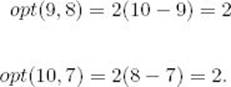
Therefore, we can compute all values in the array in Figure 3.19 by first computing all values on Diagonal 1, then computing all values on Diagonal 2, then computing all values on Diagonal 3, and so on. We illustrate the computations for the first three diagonals:

Diagonal 1:

Diagonal 2:

Diagonal 3:

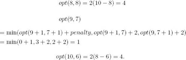
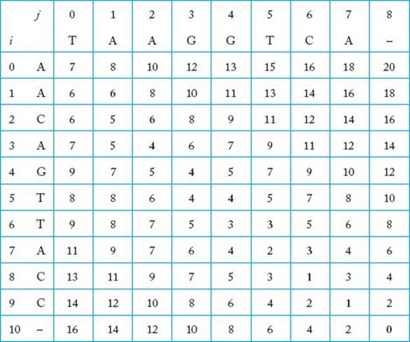
Figure 3.20 shows the array after all the values are computed. The value of the optimal alignment is opt(0, 0), which is 7.

Next, we show how the optimal alignment can be retrieved from the completed array. First, we must obtain the path that led to opt(0, 0). We do this by starting in the upper-left corner of the array and retracing our steps. We look at the three array items that could have led to opt(0, 0) and choose the one that gives the correct value. We then repeat this procedure with the chosen item. Ties are broken arbitrarily. We do this until we arrive in the lower-right corner. The path obtained is highlighted in Figure 3.20. We show how the first few values in the path were obtained. First, denote the array slot that occupies the ith row and the jth column by [i][j]. Then proceed as follows:

1. Choose array slot [0][0].

2. Find second array item in the path.

(a) Check array slot [0][1]. Since we move to the left from this slot, to arrive at array slot [0][0], a gap is inserted that means 2 is added to the cost. We have that

Figure 3.20 The completed array used to find the optimal alignment.

(b) Check array slot [1][0]. Since we move up from this slot to arrive at array slot [0][0], a gap is inserted that means 2 is added to the cost. We have that

(c) Check array slot [1][1]. Since we move diagonally from this slot to arrive at array slot [0][0], the value of penalty is added to the cost. Since x[0] = A and y[0] = T, penalty = 1. We have that

Thus, the second array slot in the path is [1][1].

Alternatively, we could create the path while storing the entries in the array. That is, each time we store an array element we create a pointer back to the array element that determined its value.

Once we have the path, we retrieve the alignment as follows (note that the sequences are generated in reverse order).

1. Starting in the bottom-right corner of the array, we follow the high-lighted path.

2. Every time we make a diagonal move to arrive at array slot [i][j], we place the character in the ith row into the x sequence and we place the character in the jth column into the y sequence.

3. Every time we make a move directly up to arrive at array slot [i][j], we place the character in the ith row into the x sequence, and we place a gap into the y sequence.

4. Every time we make a move directly to the left to arrive at array slot [i][j], we place the character in the jth column into the y sequence, and we place a gap into the x sequence.

If you follow this procedure for the array in Figure 3.20, we will obtain the following optimal alignment:

Note that if we assigned different penalties, we might obtain a different optimal alignment. Li (1997) discusses the assignment of penalties.

It is left as an exercise to write the dynamic programming algorithm for the sequence alignment problem. This algorithm for sequence alignment, which is developed in detail in Waterman (1984), is one of the most widely used sequence alignment methods. It is used in sophisticated sequence alignment systems such as BLAST (Bedell, 2003) and DASH (Gardner-Stephen and Knowles, 2004). This section is based on material in Neapolitan (2009). That text discusses molecular evolutionary genetics in much more detail.

EXERCISES

Sections 3.1

1. Establish Equality 3.1 given in this section.

2. Use induction on n to show that the divide-and-conquer algorithm for the Binomial Coefficient problem (Algorithm 3.1), based on Equality 3.1, computes terms to determine

3. Implement both algorithms for the Binomial Coefficient problem (Algorithms 3.1 and 3.2) on your system and study their performances using different problem instances.

4. Modify Algorithm 3.2 (Binomial Coefficient Using Dynamic Programming) so that it uses only a one-dimensional array indexed from 0 to k.

Sections 3.2

5. Use Floyd’s algorithm for the Shortest Paths problem 2 (Algorithm 3.4) to construct the matrix D, which contains the lengths of the shortest paths, and the matrix P, which contains the highest indices of the intermediate vertices on the shortest paths, for the following graph. Show the actions step by step.

6. Use the Print Shortest Path algorithm (Algorithm 3.5) to find the shortest path from vertex v₇ to vertex v₃, in the graph of Exercise 5, using the matrix

P found in that exercise. Show the actions step by step.

7. Analyze the Print Shortest Path algorithm (Algorithm 3.5) and show that it has a linear-time complexity.

8. Implement Floyd’s algorithm for the Shortest Paths problem 2 (Algorithm 3.4) on your system, and study its performance using different graphs.

9. Can Floyd’s algorithm for the Shortest Paths problem 2 (Algorithm 3.4) be modified to give just the shortest path from a given vertex to another specified vertex in a graph? Justify your answer.

10. Can Floyd’s algorithm for the Shortest Paths problem 2 (Algorithm 3.4) be used to find the shortest paths in a graph with some negative weights? Justify your answer.

Sections 3.3

11. Find an optimization problem in which the principle of optimality does not apply and therefore that the optimal solution cannot be obtained using dynamic programming. Justify your answer.

Sections 3.4

12. List all of the different orders in which we can multiply five matrices A, B, C, D, and E.

13. Find the optimal order, and its cost, for evaluating the product A₁ × A₂ × A₃ × A₄ × A₅, where

Show the final matrices M and P produced by Algorithm 3.6.

14. Implement the Minimum Multiplications algorithm (Algorithm 3.6) and the Print Optimal Order algorithm (Algorithm 3.7) on your system, and study their performances using different problem instances.

15. Show that a divide-and-conquer algorithm based on Equality 3.5 has an exponential-time complexity.

16. Consider the problem of determining the number of different orders in which n matrices can be multiplied.

(a) Write a recursive algorithm that takes an integer n as input and solves this problem. When n equals 1 the algorithm returns 1.

(b) Implement the algorithm and show the output of the algorithm for n = 2, 3, 4, 5, 6, 7, 8, 9, and 10.

17. Establish the equality

This is used in the every-case time complexity analysis of Algorithm 3.6.

18. Show that to fully parenthesize an expression having n matrices we need n−1 pairs of parentheses.

19. Analyze Algorithm 3.7 and show that it has a linear-time complexity.

20. Write an efficient algorithm that will find an optimal order for multiplying n matrices A₁ × A₂ × · · · × A_n, where the dimension of each matrix is 1 × 1, 1 × d, d × 1, or d × d for some positive integer d. Analyze your algorithm and show the results using order notation.

Sections 3.5

21. How many different binary search trees can be constructed using six distinct keys?

22. Create the optimal binary search tree for the following items, where the probability occurrence of each word is given in parentheses: CASE (.05), ELSE (.15), END (.05), IF (.35), OF (.05), THEN (.35).

23. Find an efficient way to compute which is used in the Optimal Binary Search Tree algorithm (Algorithm 3.9).

24. Implement the Optimal Binary Search Tree algorithm (Algorithm 3.9) and the Build Optimal Binary Search Tree algorithm (Algorithm 3.10) on your system, and study their performances using different problem instances.

25. Analyze Algorithm 3.10, and show its time complexity using order notation.

26. Generalize the Optimal Binary Search Tree algorithm (Algorithm 3.9) to the case in which the search key may not be in the tree. That is, you should let q_i, in which i = 0, 1, 2, … , n, be the probability that a missing search key can be situated between Key_i and Key_i+1. Analyze your generalized algorithm and show the results using order notation.

27. Show that a divide-and-conquer algorithm based on Equality 3.6 has an exponential time complexity.

Sections 3.6

28. Find an optimal circuit for the weighted, direct graph represented by the following matrix W. Show the actions step by step.

29. Write a more detailed version of the Dynamic Programming algorithm for the Traveling Salesperson problem (Algorithm 3.11).

30. Implement your detailed version of Algorithm 3.11 from Exercise 27 on your system and study its performance using several problem instances.

Sections 3.7

31. Analyze the time complexity of Algorithm opt, which appears in Section 3.7.

32. Write the dynamic programming algorithm for the sequence alignment problem.

33. Assuming a penalty of 1 for a mismatch and a penalty of 2 for a gap, use the dynamic programming algorithm to find an optimal alignment of the following sequences:

Additional Exercises

34. Like algorithms for computing the nth Fibonacci term (see Exercise 34 in Chapter 1), the input size in Algorithm 3.2 (Binomial Coefficient Using Dynamic Programming) is the number of symbols it takes to encode the numbers n and k. Analyze the algorithm in terms of its input size.

35. Determine the number of possible orders for multiplying n matrices A₁, A₂, … , A_n.

36. Show that the number of binary search trees with n keys is given by the formula

37. Can you develop a quadratic-time algorithm for the Optimal Binary Search Tree problem (Algorithm 3.9)?

38. Use the dynamic programming approach to write an algorithm to find the maximum sum in any contiguous sublist of a given list of n real values. Analyze your algorithm, and show the results using order notation.

39. Let us consider two sequences of characters S₁ and S₂. For example, we could have S₁ = A$CMA*MN and S₂ = AXMC4ANB. Assuming that a subsequence of a sequence can be constructed by deleting any number of characters from any positions, use the dynamic programming approach to create an algorithm that finds the longest common subsequence of S₁ and S₂. This algorithm returns the maximum-length common subsequence of each sequence.