Foundations of Algorithms (2015)

Chapter 4 The Greedy Approach

Charles Dickens’ classic character Ebenezer Scrooge may well be the most greedy person ever, fictional or real. Recall that Scrooge never considered the past or future. Each day his only drive was to greedily grab as much gold as he could. After the Ghost of Christmas Past reminded him of the past and the Ghost of Christmas Future warned him of the future, he changed his greedy ways.

A greedy algorithm proceeds in the same way as Scrooge did. That is, it grabs data items in sequence, each time taking the one that is deemed “best” according to some criterion, without regard for the choices it has made before or will make in the future. One should not get the impression that there is something wrong with greedy algorithms because of the negative connotations of Scrooge and the word “greedy.” They often lead to very efficient and simple solutions.

Like dynamic programming, greedy algorithms are often used to solve optimization problems. However, the greedy approach is more straightforward. In dynamic programming, a recursive property is used to divide an instance into smaller instances. In the greedy approach, there is no division into smaller instances. A greedy algorithm arrives at a solution by making a sequence of choices, each of which simply looks the best at the moment. That is, each choice is locally optimal. The hope is that a globally optimal solution will be obtained, but this is not always the case. For a given algorithm, we must determine whether the solution is always optimal.

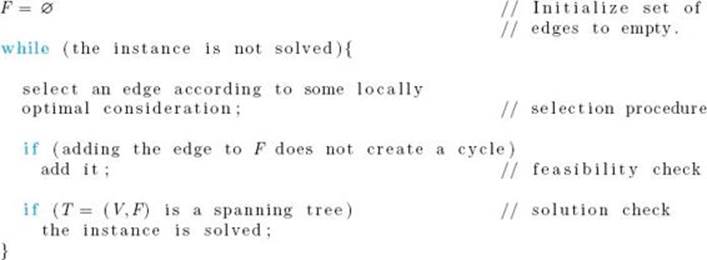
A simple example illustrates the greedy approach. Joe, the sales clerk, often encounters the problem of giving change for a purchase. Customers usually don’t want to receive a lot of coins. For example, most customers would be aggravated if he gave them 87 pennies when the change was $0.87. Therefore, his goal is not only to give the correct change, but to do so with as few coins as possible. A solution to an instance of Joe’s change problem is a set of coins that adds up to the amount he owes the customer, and an optimal solution is such a set of minimum size. A greedy approach to the problem could proceed as follows. Initially there are no coins in the change. Joe starts by looking for the largest coin (in value) he can find. That is, his criterion for deciding which coin is best (locally optimal) is the value of the coin. This is called the selection procedure in a greedy algorithm. Next he sees if adding this coin to the change would make the total value of the change exceed the amount owed. This is called the feasibility check in a greedy algorithm. If adding the coin would not make the change exceed the amount owed, he adds the coin to the change. Next he checks to see if the value of the change is now equal to the amount owed. This is the solution check in a greedy algorithm. If the values are not equal, Joe gets another coin using his selection procedure and repeats the process. He does this until the value of the change equals the amount owed or he runs out of coins. In the latter case, he is not able to return the exact amount owed. The following is a high-level algorithm for this procedure.

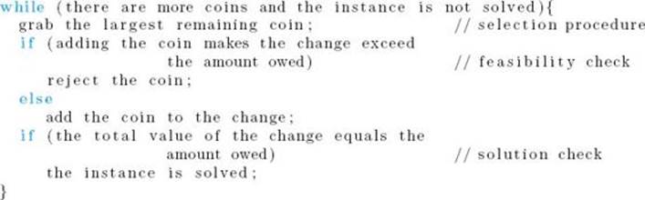
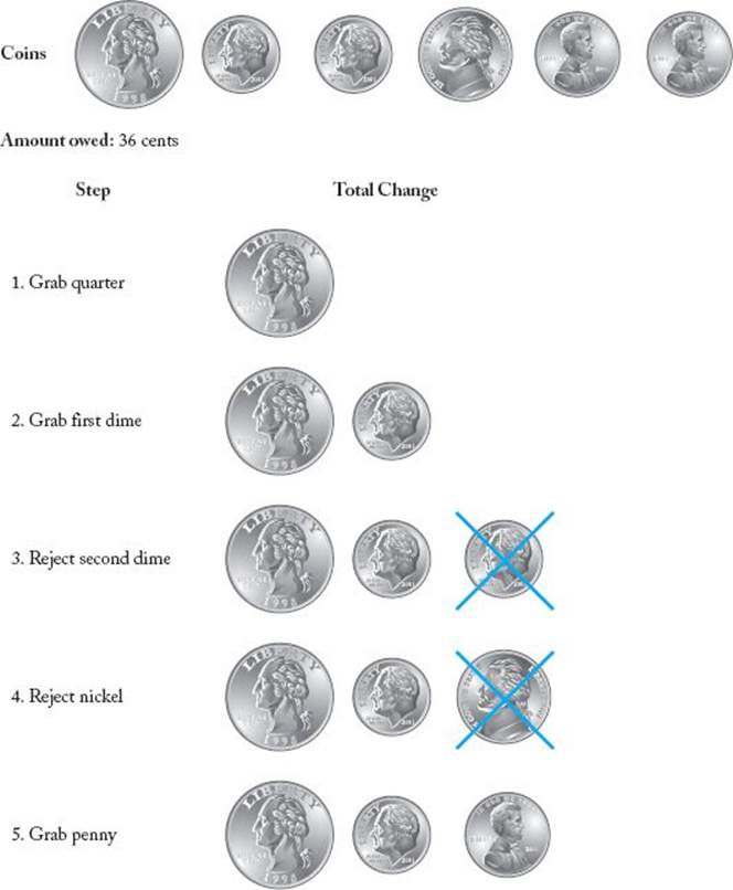
In the feasibility check, when we determine that adding a coin would make the change exceed the amount owed, we learn that the set obtained by adding that coin cannot be completed to give a solution to the instance. Therefore, that set is unfeasible and is rejected. An example application of this algorithm appears in Figure 4.1. Again, the algorithm is called “greedy” because the selection procedure simply consists of greedily grabbing the next-largest coin without considering the potential drawbacks of making such a choice. There is no opportunity to reconsider a choice. Once a coin is accepted, it is permanently included in the solution; once a coin is rejected, it is permanently excluded from the solution. This procedure is very simple, but does it result in an optimal solution? That is, in the Change problem, when a solution is possible, does the solution provided by the algorithm contain the minimum number of coins necessary to give the correct change? If the coins consist of U.S. coins (penny, nickel, dime, quarter, half dollar) and if there is at least one type of each coin available, the greedy algorithm always returns an optimal solution when a solution exists. This is proven in the exercises. There are cases other than those involving standard U.S. coins for which the greedy algorithm produces optimal solutions. Some of these also are investigated in the exercises. Notice here that if we include a 12-cent coin with the U.S. coins, the greedy algorithm does not always give an optimal solution. Figure 4.2 illustrates this result. In that figure, the greedy solution contains five coins, whereas the optimal solution, which consists of a dime, nickel, and penny, contains only three coins.

Figure 4.1 A greedy algorithm for giving change.

As this Change problem shows, a greedy algorithm does not guarantee an optimal solution. We must always determine whether this is the case for a particular greedy algorithm. Sections 4.1, 4.2, 4.3, and 4.4 discuss problems for which the greedy approach always yields an optimal solution. Section 4.5 investigates a problem in which it does not. In that section, we compare the greedy approach with dynamic programming to illuminate when each approach might be applicable. We close here with a general outline of the greedy approach. A greedy algorithm starts with an empty set and adds items to the set in sequence until the set represents a solution to an instance of a problem. Each iteration consists of the following components:

Figure 4.2 The greedy algorithm is not optimal if a 12-cent coin is included.

• A selection procedure chooses the next item to add to the set. The selection is performed according to a greedy criterion that satisfies some locally optimal consideration at the time.

• A feasibility check determines if the new set is feasible by checking whether it is possible to complete this set in such a way as to give a solution to the instance.

• A solution check determines whether the new set constitutes a solution to the instance.

4.1 Minimum Spanning Trees

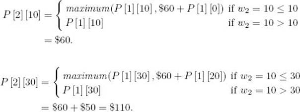
Suppose an urban planner wants to connect certain cities with roads so that it is possible for someone to drive from any city to any other city. If there are budgetary restrictions, the planner may want to do this with the minimum amount of road. We will develop an algorithm that solves this and similar problems. First, let’s informally review more graph theory. Figure 4.3(a) shows a connected, weighted, undirected graph G. We assume here that the weights are nonnegative numbers. The graph is undirected because the edges do not have direction. This is represented pictorially by an absence of arrows on the edges. Because the edges do not have direction, we say an edge is between two vertices. A path in an undirected graph is a sequence of vertices such that there is an edge between each vertex and its successor. Because the edges have no direction, there is a path from vertex u to vertex v if and only if there is a path from v to u. Therefore, for undirected graphs we simply say that there is a path between two vertices. An undirected graph is called connected if there is a path between every pair of vertices. All the graphs in Figure 4.3 are connected. If we removed the edge between v₂ and v₄ from the graph in Figure 4.3(b), the graph would no longer be connected.

Figure 4.3 A weighted graph and three subgraphs.

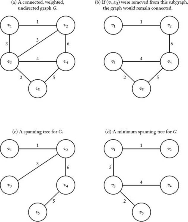
In an undirected graph, a path from a vertex to itself, which contains at least three vertices and in which all intermediate vertices are distinct, is called a simple cycle. An undirected graph with no simple cycles is called acyclic. The graphs in Figure 4.3(c) and (d) are acyclic, whereas the ones inFigure 4.3(a) and (b) are not. A tree (technically, a free tree) is an acyclic, connected, undirected graph. The graphs in Figure 4.3(c) and (d) are trees. With this definition, no vertex is singled out as the root, and a rooted tree is defined as a tree with one vertex designated as the root. Therefore, a rooted tree is what is often called a tree (as was done in Section 3.5).

Consider the problem of removing edges from a connected, weighted, undirected graph G to form a subgraph such that all the vertices remain connected and the sum of the weights on the remaining edges is as small as possible. Such a problem has numerous applications. As mentioned earlier, in road construction we may want to connect a set of cities with a minimum amount of road. Similarly, in telecommunications we may want to use a minimal length of cable, and in plumbing we may want to use a minimal amount of pipe. A subgraph with minimum weight must be a tree, because if a subgraph were not a tree, it would contain a simple cycle, and we could remove any edge on the cycle, resulting in a connected graph with a smaller weight. To illustrate this, look at Figure 4.3. The subgraph in Figure 4.3(b) of the graph in Figure 4.3(a) cannot have minimum weight because if we remove any edge on the simple cycle [v₃, v₄, v₅, v₃], the subgraph remains connected. For example, we could remove the edge connecting v₄ and v₅, resulting in a connected graph with a smaller weight.

A spanning tree for G is a connected subgraph that contains all the vertices in G and is a tree. The trees in Figure 4.3(c) and (d) are spanning trees for G. A connected subgraph of minimum weight must be a spanning tree, but not every spanning tree has minimum weight. For example, the spanning tree in Figure 4.3(c) does not have mininum weight, because the spanning tree in Figure 4.3(d) has a lesser weight. An algorithm for our problem must obtain a spanning tree of minimum weight. Such a tree is called a minimum spanning tree. The tree in Figure 4.3(d) is a minimum spanning tree for G. A graph can have more than one minimum spanning tree. There is another one for G, which you may wish to find.

To find a minimum spanning tree by the brute-force method of considering all spanning trees is worse than exponential in the worst case. We will solve the problem more efficiently using the greedy approach. First we need the formal definition of an undirected graph.

Definition

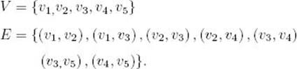
An undirected graph G consists of a finite set V whose members are called the vertices of G, together with a set E of pairs of vertices in V. These pairs are called the edges of G. We denote G by

We will denote members of V by v_i and the edge between v_i and v_j by

Example 4.1

For the graph in Figure 4.3(a),

The order in which we list the vertices to denote an edge is irrelevant in an undirected graph. For example, (v₁, v₂) denotes the same edge as (v₂, v₁). We have listed the vertex with the lower index first.

A spanning tree T for G has the same vertices V as G, but the set of edges of T is a subset F of E. We will denote a spanning tree by T = (V , F). Our problem is to find a subset F of E such that T = (V , F) is a minimum spanning tree for G. A high-level greedy algorithm for the problem could proceed as follows:

This algorithm simply says “select an edge according to some locally optimal consideration.” There is no unique locally optimal property for a given problem. We will investigate two different greedy algorithms for this problem, Prim’s algorithm and Kruskal’s algorithm. Each uses a different locally optimal property. Recall that there is no guarantee that a given greedy algorithm always yields an optimal solution. One must prove whether or not this is the case. We will prove that both Prim’s and Kruskal’s algorithms always produce minimum spanning trees.

• 4.1.1 Prim’s Algorithm

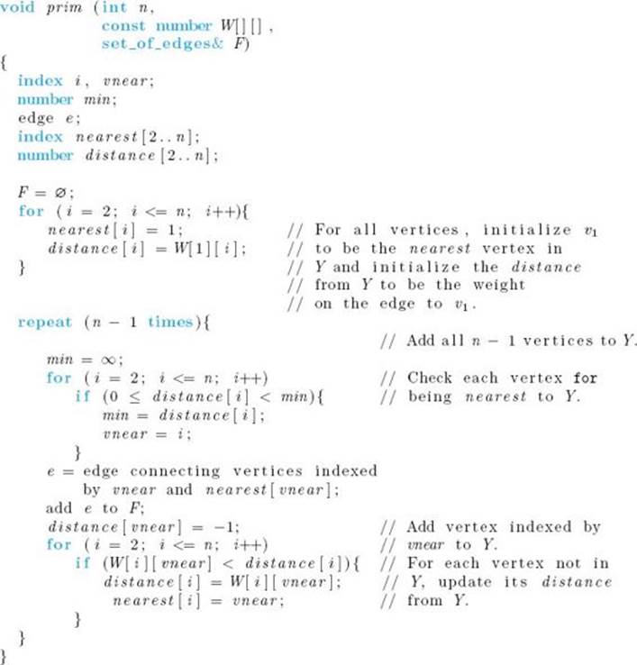
Prim’s algorithm starts with an empty subset of edges F and a subset of vertices Y initialized to contain an arbitrary vertex. We will initialize Y to {v₁}. A vertex nearest to Y is a vertex in V −Y that is connected to a vertex in Y by an edge of minimum weight. (Recall from Chapter 3 that weight and distance terminology are used interchangeably for weighted graphs.) In Figure 4.3(a), v₂ is nearest to Y when Y = {v₁}. The vertex that is nearest to Y is added to Y and the edge is added to F. Ties are broken arbitrarily. In this case, v₂ is added to Y, and (v₁, v₂) is added to F. This process of adding nearest vertices is repeated until Y = V . The following is a high-level algorithm for this procedure:

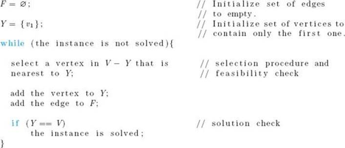
The selection procedure and feasibility check are done together because taking the new vertex from V − Y guarantees that a cycle is not created. Figure 4.4 illustrates Prim’s algorithm. At each step in that figure, Y contains the shaded vertices and F contains the shaded edges.

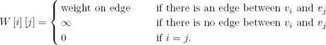
The high-level algorithm works fine for a human creating a minimum spanning tree for a small graph from a picture of the graph. The human merely finds the vertex nearest to Y by inspection. However, for the purposes of writing an algorithm that can be implemented in a computer language,we need to describe a step-by-step procedure. To this end, we represent a weighted graph by its adjacency matrix. That is, we represent it by an n × n array W of numbers where

Figure 4.4 A weighted graph (in upper-left corner) and the steps in Prim’s algorithm for that graph. The vertices in Y and the edges in F are shaded at each step.

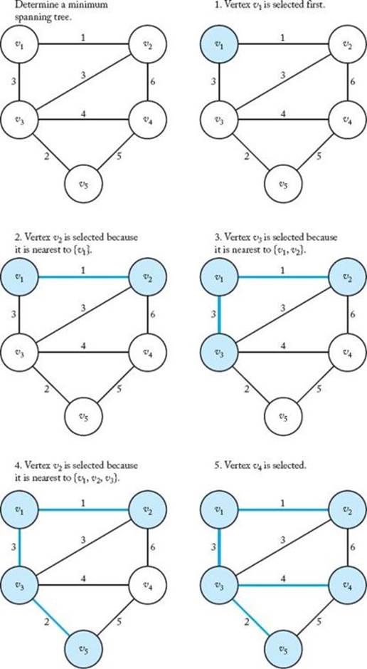
Figure 4.5 The array representation W of the graph in Figure 4.3(a).

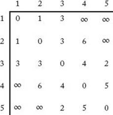
The graph in Figure 4.3(a) is represented in this manner in Figure 4.5. We maintain two arrays, nearest and distance, where, for i = 2, … , n,

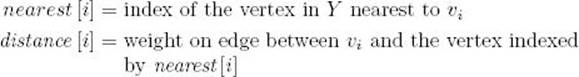
Because at the start Y = {v₁}, nearest[i] is initialized to 1 and distance[i] is initialized to the weight on the edge between v₁ and v_i. As vertices are added to Y , these two arrays are updated to reference the new vertex in Y nearest to each vertex outside of Y . To determine which vertex to add to Y , in each iteration we compute the index for which distance[i] is the smallest. We call this index vnear. The vertex indexed by vnear is added to Y by setting distance[vnear] to −1. The following algorithm implements this procedure.

Algorithm 4.1

Prim’s Algorithm

Problem: Determine a minimum spanning tree.

Inputs: integer n ≥ 2, and a connected, weighted, undirected graph containing n vertices. The graph is represented by a two-dimensional array W, which has both its rows and columns indexed from 1 to n, where W [i] [j] is the weight on the edge between the ith vertex and the jth vertex.

Outputs: set of edges F in a minimum spanning tree for the graph.

Analysis of Algorithm 4.1

Every-Case Time Complexity (Prim’s Algorithm)

Basic operation: There are two loops, each with n−1 iterations, inside the repeat loop. Executing the instructions inside each of them can be considered to be doing the basic operation once.

Input size: n, the number of vertices.

Because the repeat loop has n − 1 iterations, the time complexity is given by

Clearly, Prim’s algorithm produces a spanning tree. However, is it necessarily minimal? Because at each step we select the vertex nearest to Y , intuitively it seems that the tree should be minimal. However, we need to prove whether or not this is the case. Although greedy algorithms are often easier to develop than dynamic programming algorithms, usually it is more difficult to determine whether or not a greedy algorithm always produces an optimal solution. Recall that for a dynamic programming algorithm we need only show that the principle of optimality applies. For a greedy algorithm we usually need a formal proof. Next we give such a proof for Prim’s algorithm.

Let an undirected graph G = (V , E) be given. A subset F and E is called promising if edges can be added to it so as to form a minimum spanning tree. The subset {(v₁, v₂) , (v₁, v₃)}, in Figure 4.3(a) is promising, and the subset {(v₂, v₄)} is not promising.

Lemma 4.1

Let G = (V , E) be a connected, weighted, undirected graph; let F be a promising subset of E; and let Y be the set of vertices connected by the edges in F. If e is an edge of minimum weight that connects a vertex in Y to a vertex in V − Y , then F ∪ {e} is promising.

Proof: Because F is promising, there must be some set of edges F′ such that

and (V , F′) is a minimum spanning tree. If e ∈ F′, then

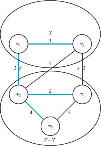
which means F ∪ {e} is promising and we’re done. Otherwise, because (V , F′) is a spanning tree, F′ ∪ {e} must contain exactly one simple cycle and e must be in the cycle. Figure 4.6 illustrates this. The simple cycle is [v₁, v₂, v₄, v₃]. As can be seen in Figure 4.6, there must be another edge e′∈ F′ in the simple cycle that also connects a vertex in Y to one in V −Y . If we remove e′ from F′ ∪ {e}, the simple cycle disappears, which means that we have a spanning tree. Because e is an edge of minimum weight that connects a vertex in Y to one in V − Y , the weight of e must be less than or equal to the weight of e′(in fact, they must be equal). So

Figure 4.6 A graph illustrating the proof in Lemma 4.1. The edges in F′ are shaded in color.

is a minimum spanning tree. Now

because e′ cannot be in F (recall that edges in F connect only vertices in Y .) Therefore, F ∪ {e} is promising, which completes the proof.

Theorem 4.1

Prim’s algorithm always produces a minimum spanning tree.

Proof: We use induction to show that the set F is promising after each iteration of the repeat loop.

Induction base: Clearly the empty set ∅ is promising.

Induction hypothesis: Assume that, after a given iteration of the repeat loop, the set of edges so far selected—namely, F—is promising.

Induction step: We need to show that the set F ∪ {e} is promising, where e is the edge selected in the next iteration. Because the edge e selected in the next iteration is an edge of minimum weight that connects a vertex in Y to one on V − Y , F ∪ {e} is promising, by Lemma 4.1. This completes the induction proof.

By the induction proof, the final set of edges is promising. Because this set consists of the edges in a spanning tree, that tree must be a minimum spanning tree.

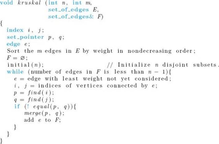
• 4.1.2 Kruskal’s Algorithm

Kruskal’s algorithm for the Minimum Spanning Tree problem starts by creating disjoint subsets of V , one for each vertex and containing only that vertex. It then inspects the edges according to nondecreasing weight (ties are broken arbitrarily). If an edge connects two vertices in disjoint subsets, the edge is added and the subsets are merged into one set. This process is repeated until all the subsets are merged into one set. The following is a high-level algorithm for this procedure.

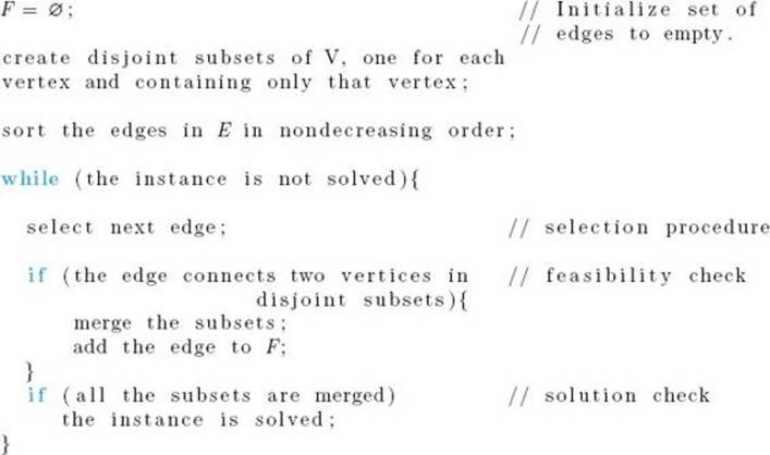
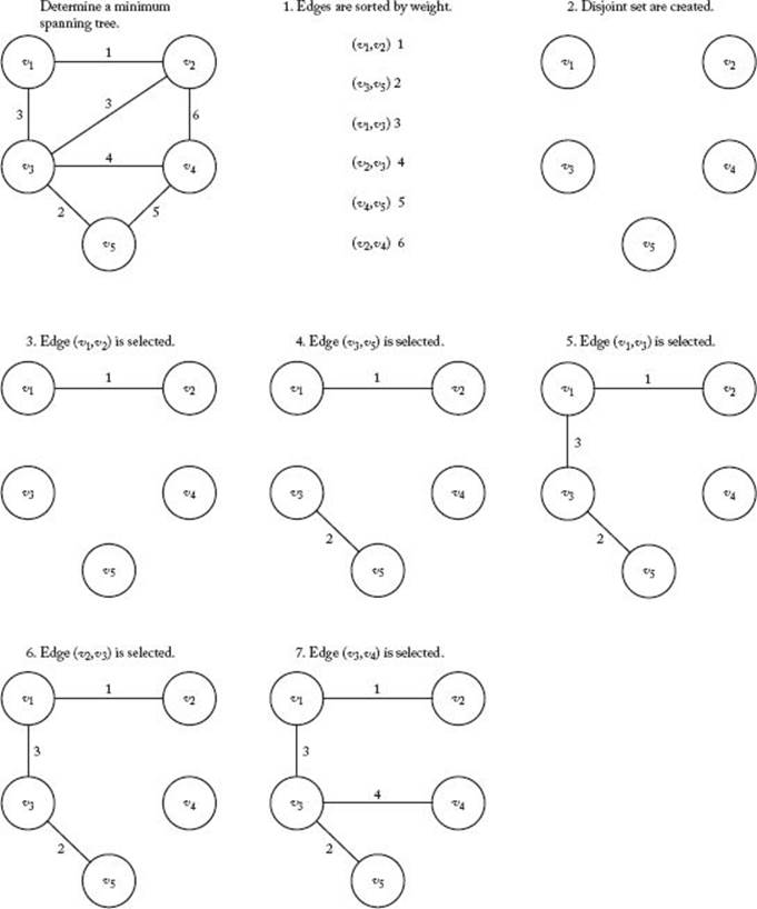
Figure 4.7 illustrates Kruskal’s algorithm.

To write a formal version of Kruskal’s algorithm, we need a disjoint set abstract data type. Such a data type is implemented in Appendix C. Because that implementation is for disjoint subsets of indices, we need only refer to the vertices by index to use the implementation. The disjoint set abstract data type consists of data types index and set pointer, and routines initial, find, merge, and equal, such that if we declare

Figure 4.7 A weighted graph (in upper-left corner) and the steps in Kruskal’s algorithm for that graph.

then

• initial(n) initializes n disjoint subsets, each of which contains exactly one of the indices between 1 and n.

• p = find(i) makes p point to the set containing index i.

• merge(p, q) merges the two sets, to which p and q point, into the set.

• equal(p, q) returns true if p and q both point to the same set.

The algorithm follows.

Algorithm 4.2

Kruskal’s Algorithm

Problem: Determine a minimum spanning tree.

Inputs: integer n ≥ 2, positive integer m, and a connected, weighted, undirected graph containing n vertices and m edges. The graph is represented by a set E that contains the edges in the graph along with their weights.

Outputs: F, a set of edges in a minimum spanning tree.

The while loop is exited when there are n−1 edges in F, because there are n − 1 edges in a spanning tree.

Analysis of Algorithm 4.2

Worst-Case Time-Complexity (KruskaI’s Algorithm)

Basic operation: a comparison instruction.

Input size: n, the number of vertices, and m, the number of edges.

There are three considerations in this algorithm:

1. The time to sort the edges. We obtained a sorting algorithm in Chapter 2 (Mergesort) that is worst-case Θ(m lg m). In Chapter 7 we will show, for algorithms that sort by comparison of keys, that it is not possible to improve on this performance. Therefore, the time complexity for sorting the edges is given by

2. The time in the while loop. The time it takes to manipulate the disjoint sets is dominant in this loop (because everything else is constant). In the worst case, every edge is considered before the while loop is exited, which means there are m passes through the loop. Using the implementation called Disjoint Set Data Structure II in Appendix C, the time complexity for m passes through a loop that contains a constant number of calls to routines find, equal, and merge is given by

where the basic operation is a comparison instruction.

3. The time to initialize n disjoint sets. Using the disjoint set data structure implementation mentioned previously, the time complexity for the initialization is given by

Because m ≥ n−1, the sorting and the manipulations of the disjoint sets dominate the initialization time, which means that

It may appear that the worst case has no dependence on n. However, in the worst case, every vertex can be connected to every other vertex, which would mean that

Therefore, we can also write the worst case as follows:

It is useful to use both expressions for the worst case when comparing Kruskal’s algorithm with Prim’s algorithm.

We need the following lemma to prove that Kruskal’s algorithm always produces an optimal solution.

Lemma 4.2

Let G = (V , E) be a connected, weighted, undirected graph; let F be a promising subset of E; and let e be an edge of minimum weight in E − F such that F ∪ {e} has no simple cycles. Then F ∪ {e} is promising.

Proof: The proof is similar to the proof of Lemma 4.1. Because F is promising, there must be some set of edges F′ such that

and (V , F′) is a minimum spanning tree. If e ∈ F′, then

which means that F ∪ {e} is promising and we’re done. Otherwise, because (V , F′) is a spanning tree, F′ ∪ {e} must contain exactly one simple cycle and e must be in the cycle. Because F ∪{e} contains no simple cycles, there must be some edge e′ ∈ F′ that is in the cycle and that is not in F. That is, e′ ∈ E − F . The set F ∪ {e′} has no simple cycles because it is a subset of F′. Therefore, the weight of e is no greater than the weight of e′. (Recall that we assumed e is an edge of minimum weight in E − F such that F ∪{e} has no cycles.) If we remove e′ from F′ ∪ {e}, the simple cycle in this set disappears, which means we have a spanning tree. Indeed

is a minimum spanning tree because, as we have shown, the weight of e is no greater than the weight of e′. Because e′ is not in F,

Therefore, F ∪ {e} is promising, which completes the proof.

Theorem 4.2

Kruskal’s algorithm always produces a minimum spanning tree.

Proof: The proof is by induction, starting with the empty set of edges. You are asked to apply Lemma 4.2 to complete the proof in the exercises.

• 4.1.3 Comparing Prim’s Algorithm with Kruskal’s Algorithm

We obtained the following time complexities:

Prim’s Algorithm: T(n) ∈ Θ(n²)

Kruskal’s Algorithm: W (m, n) ∈ Θ(m lg m) and W (m, n) ∈ Θ(n² lg n)

We also showed that in a connected graph

For a graph whose number of edges m is near the low end of these limits (the graph is very sparse), Kruskal’s algorithm is Θ(n lg n), which means that Kruskal’s algorithm should be faster. However, for a graph whose number of edges is near the high end (the graph is highly connected), Kruskal’s algorithm is Θ(n² lg n)_, which means that Prim’s algorithm should be faster.

• 4.1.4 Final Discussion

As mentioned before, the time complexity of an algorithm sometimes depends on the data structure used to implement it. Using heaps, Johnson (1977) created a Θ(m lg n) implementation of Prim’s algorithm. For a sparse graph, this is Θ(n lg n), which is an improvement over our implementation. But for a dense graph, it is Θ(n² lg n)_, which is slower than our implementation. Using the Fibonacci heap, Fredman and Tarjan (1987) developed the fastest implementation of Prim’s algorithm. Their implementation is Θ(m + n lg n). For a sparse graph, this is Θ(n lg n), and for a dense graph it is Θ(n²) _.

Prim’s algorithm originally appeared in Jarník (1930) and was published by its namesake in Prim (1957). Kruskal’s algorithm is from Kruskal (1956). The history of the Minimum Spanning Tree problem is discussed in Graham and Hell (1985). Other algorithms for the problem can be found in Yao (1975) and Tarjan (1983).

4.2 Dijkstra’s Algorithm for Single-Source Shortest Paths

In Section 3.2, we developed a Θ(n³) algorithm for determining the shortest paths from each vertex to all other vertices in a weighted, directed graph. If we wanted to know only the shortest paths from one particular vertex to all the others, that algorithm would be overkill. Next we will use the greedy approach to develop a Θ(n²) algorithm for this problem (called the Single-Source Shortest Paths problem). This algorithm is due to Dijkstra (1959). We present the algorithm, assuming that there is a path from the vertex of interest to each of the other vertices. It is a simple modification to handle the case where this is not so.

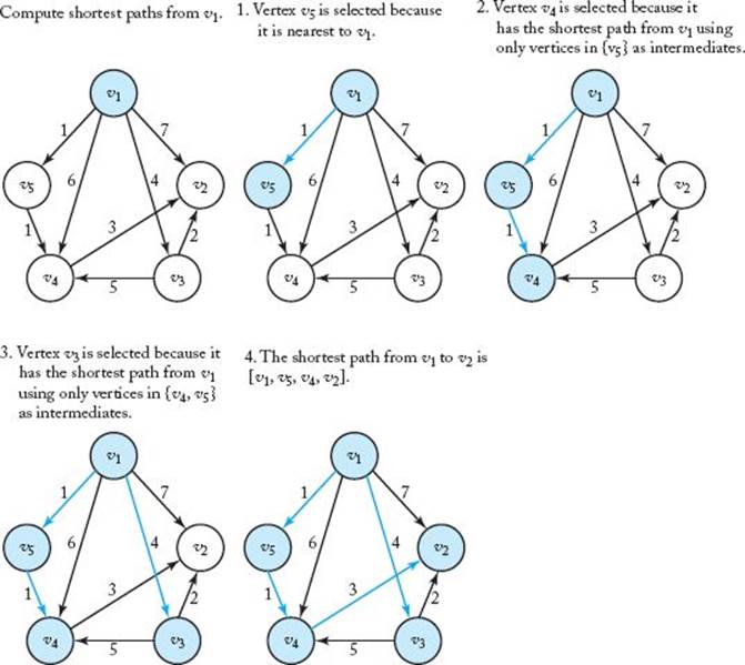
This algorithm is similar to Prim’s algorithm for the Minimum Spanning Tree problem. We initialize a set Y to contain only the vertex whose shortest paths are to be determined. For focus, we say that the vertex is v₁. We initialize a set F of edges to being empty. First we choose a vertex v that isnearest to v₁, add it to Y , and add the edge < v₁, v > to F. (By < v₁, v > we mean the directed edge from v₁ to v.) That edge is clearly a shortest path from v₁ to v. Next we check the paths from v₁ to the vertices in V − Y that allow only vertices in Y as intermediate vertices. A shortest of these paths is a shortest path (this needs to be proven). The vertex at the end of such a path is added to Y , and the edge (on the path) that touches that vertex is added to F. This procedure is continued until Y equals V , the set of all vertices. At this point, F contains the edges in shortest paths. The following is a high-level algorithm for this approach.

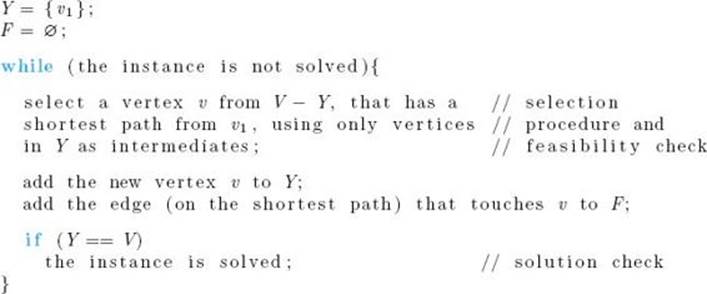
Figure 4.8 illustrates Dijkstra’s algorithm. As was the case for Prim’s algorithm, the high-level algorithm works only for a human solving an instance by inspection on a small graph. Next we give a detailed algorithm. For this algorithm, the weighted graph is represented by a two-dimensional array exactly as was done in Section 3.2. This algorithm is very similar to Algorithm 4.1 (Prim’s). The difference is that instead of the arrays nearest and distance, we have arrays touch and length, where for i = 2, … , n,

touch[i] = index of vertex v in Y such that the edge <v, v_i> is the last edge on the current shortest path from v₁ to v_i using only vertices in Y as intermediates.

length[i] = length of the current shortest path from v₁ to v_i using only vertices in Y as intermediates.

The algorithm follows.

Algorithm 4.3

Dijkstra’s Algorithm

Problem: Determine the shortest paths from v₁ to all other vertices in a weighted, directed graph.

Inputs: integer n ≥ 2, and a connected, weighted, directed graph containing n vertices. The graph is represented by a two-dimensional array W, which has both its rows and columns indexed from 1 to n, where W [i] [j] is the weight on the edge from the ith vertex to the jth vertex.

Figure 4.8 A weighted, directed graph (in upper-left corner) and the steps in Dijkstra’s algorithm for that graph. The vertices in Y and the edges in F are shaded in color at each step.

Outputs: set of edges F containing edges in shortest paths.

Because we are assuming that there is a path from v₁ to every other vertex, the variable vnear has a new value in each iteration of the repeat loop. If this were not the case, the algorithm, as written, would end up adding the last edge over and over until n − 1 iterations of the repeat loop were completed.

Algorithm 4.3 determines only the edges in the shortest paths. It does not produce the lengths of those paths. These lengths could be obtained from the edges. Alternatively, a simple modification of the algorithm would enable it to compute the lengths and store them in an array as well.

The control in Algorithm 4.3 is identical to that in Algorithm 4.1. Therefore, from the analysis of that Algorithm 4.1, we know for Algorithm 4.3 that

Although we do not do it here, it is possible to prove that Algorithm 4.3 always produces shortest paths. The proof uses an induction argument similar to the one used to prove that Prim’s algorithm (Algorithm 4.1) always produces a minimum spanning tree.

As is the case for Prim’s algorithm, Dijkstra’s algorithm can be implemented using a heap or a Fibonacci heap. The heap implementation is Θ(m lg n), and the Fibonacci heap implementation is Θ(m + n lg n), where m is the number of edges. See Fredman and Tarjan (1987) for this latter implementation.

4.3 Scheduling

Suppose a hair stylist has several customers waiting for different treatments (e.g., simple cut, cut with shampoo, permanent, hair coloring). The treatments don’t all take the same amount of time, but the stylist knows how long each takes. A reasonable goal would be to schedule the customers in such a way as to minimize the total time they spend both waiting and being served (getting treated). Such a schedule is considered optimal. The time spent both waiting and being served is called the time in the system. The problem of minimizing the total time in the system has many applications. For example, we may want to schedule users’ access to a disk drive to minimize the total time they spend waiting and being served.

Another scheduling problem occurs when each job (customer) takes the same amount of time to complete but has a deadline by which it must start to yield a profit associated with the job. The goal is to schedule the jobs to maximize the total profit. We will consider scheduling with deadlinesafter discussing the simpler scheduling problem of minimizing the total time in the system.

• 4.3.1 Minimizing Total Time in the System

A simple solution to minimizing the total time in the system is to consider all possible schedules and take the minimum. This is illustrated in the following example.

Example 4.2

Suppose there are three jobs and the service times for these jobs are

The actual time units are not relevant to the problem. If we schedule them in the order 1, 2, 3, the times spent in the system for the three jobs are as follows:

The total time in the system for this schedule is

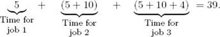
This same method of computation yields the following list of all possible schedules and total times in the system:

Schedule [3, 1, 2] is optimal with a total time of 32.

Clearly, an algorithm that considers all possible schedules is factorialtime. Notice in the previous example that an optimal schedule occurs when the job with the smallest service time (job 3, with a service time of 4) is scheduled first, followed by the job with the second-smallest service time (job 1, with a service time of 5), followed finally by the job with the largest service time (job 2, with a service time of 10). Intuitively, it seems that such a schedule would be optimal because it gets the shortest jobs out of the way first. A high-level greedy algorithm for this approach is as follows:

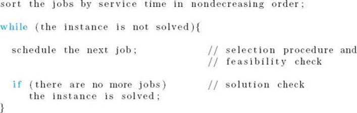
We wrote this algorithm in the general form of the greedy approach to show that it is indeed a greedy algorithm. However, clearly all the algorithm does is sort the jobs according to service time. Its time complexity is therefore given by

Although intuitively it seems that the schedule created by this algorithm is optimal, this supposition needs to be proved. The following theorem proves the stronger result that this schedule is the only optimal one.

Theorem 4.3

The only schedule that minimizes the total time in the system is one that schedules jobs in nondecreasing order by service time.

Proof: For 1 ≤ i ≤ n − 1, let t_i be the service time for the ith job scheduled in some particular optimal schedule (one that minimizes the total time in the system). We need to show that the schedule has the jobs scheduled in nondecreasing order by service time. We show this using proof by contradiction. If they are not scheduled in nondecreasing order, then for at least one i where 1 ≤ i ≤ n − 1,

We can rearrange our original schedule by interchanging the ith and (i + 1)st jobs. By doing this, we have taken t_i units off the time the (i + 1)st job (in the original schedule) spends in the system. The reason is that it no longer waits while the ith job (in the original schedule) is being served. Similarly, we have added t_i+1 units to the time the ith job (in the original schedule) spends in the system. Clearly, we have not changed the time that any other job spends in the system. Therefore, if T is the total time in the system in our original schedule and T′ is the total time in the rearranged schedule,

Because t_i > t_i+1,

which contradicts the optimality of our original schedule.

It is straightforward to generalize our algorithm to handle the Multiple-Server Scheduling problem. Suppose there are m servers. Order those servers in an arbitrary manner. Order the jobs again by service time in nondecreasing order. Let the first server serve the first job, the second server the second job, … , and the mth server the mth job. The first server will finish first because that server serves the job with the shortest service time. Therefore, the first server serves the (m + 1)st job. Similarly, the second server serves the (m + 2)nd job, and so on. The scheme is as follows:

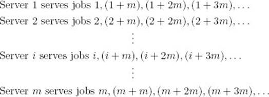
Clearly, the jobs end up being processed in the following order:

That is, the jobs are processed in nondecreasing order by service time.

• 4.3.2 Scheduling with Deadlines

In this scheduling problem, each job takes one unit of time to finish and has a deadline and a profit. If the job starts before or at its deadline, the profit is obtained. The goal is to schedule the jobs so as to maximize the total profit. Not all jobs have to be scheduled. We need not consider any schedule that has a job scheduled after its deadline because that schedule has the same profit as one that doesn’t schedule the job at all. We call such a schedule impossible. The following example illustrates this problem.

Example 4.3

Suppose we have the following jobs, deadlines, and profits:

When we say that job 1 has a deadline of 2, we mean that job 1 can start at time 1 or time 2. There is no time 0. Because job 2 has a deadline of 1, that job can start only at time 1. The possible schedules and total profits are as follows:

Impossible schedules have not been listed. For example, schedule [1, 2] is not possible, and is therefore not listed, because job 1 would start first at time 1 and take one unit of time to finish, causing job 2 to start at time 2. However, the deadline for job 2 is time 1. Schedule [1, 3], for example, is possible because job 1 is started before its deadline, and job 3 is started at its deadline. We see that schedule [4, 1] is optimal with a total profit of 70.

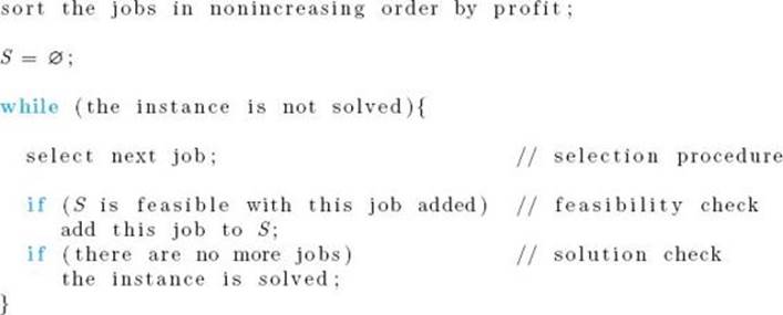
To consider all schedules, as is done in Example 4.3, takes factorial time. Notice in the example that the job with the greatest profit (job 4) is included in the optimal schedule, but the job with the second-greatest profit (job 2) is not. Because both jobs have deadlines equal to 1, both cannot be scheduled. Of course, the one with the greatest profit is the one scheduled. The other job scheduled is job 1, because its profit is greater than that of job 3. This suggests that a reasonable greedy approach to solving the problem would be to first sort the jobs in nonincreasing order by profit, and next inspect each job in sequence and add it to the schedule if it is possible. Before we can create even a high-level algorithm for this approach, we need some definitions.

A sequence is called a feasible sequence if all the jobs in the sequence start by their deadlines. For example, [4, 1] is a feasible sequence in Example 4.3, but [1, 4] is not a feasible sequence. A set of jobs is called a feasible set if there exists at least one feasible sequence for the jobs in the set. In Example 4.3, {1, 4} is a feasible set because the scheduling sequence [4, 1] is feasible, whereas {2, 4} is not a feasible set because no scheduling sequence allows both jobs to start by their deadlines. Our goal is to find a feasible sequence with maximum total profit. We call such a sequence anoptimal sequence and the set of jobs in the sequence an optimal set of jobs. We can now present a high-level greedy algorithm for the Scheduling with Deadlines problem.

The following example illustrates this algorithm.

Example 4.4

Suppose we have the following jobs, deadlines, and profits:

We have already sorted the jobs before labeling them. The previous greedy algorithm does the following:

1. S is set to ∅.

2. S is set to {1} because the sequence [1] is feasible.

3. S is set to {1, 2} because the sequence [2, 1] is feasible.

4. {1, 2, 3} is rejected because there is no feasible sequence for this set. 5. S is set to {1, 2, 4} because the sequence [2, 1, 4] is feasible.

6. {1, 2, 4, 5} is rejected because there is no feasible sequence for this set.

7. {1, 2, 4, 6} is rejected because there is no feasible sequence for this set.

8. {1, 2, 4, 7} is rejected because there is no feasible sequence for this set.

The final value of S is {1, 2, 4}, and a feasible sequence for this set is [2, 1, 4]. Because jobs 1 and 4 both have deadlines of 3, we could use the feasible sequence [2, 4, 1] instead.

Before proving that this algorithm always produces an optimal sequence, let’s write a formal version of it. To do this, we need an efficient way to determine whether a set is feasible. To consider all possible sequences is not acceptable because it would take factorial time to do this. The following lemma enables us to check efficiently whether or not a set is feasible.

Lemma 4.3

Let S be a set of jobs. Then S is feasible if and only if the sequence obtained by ordering the jobs in S according to nondecreasing deadlines is feasible.

Proof: Suppose S is feasible. Then there exists at least one feasible sequence for the jobs in S. In this sequence, suppose that job x is scheduled before job y, and job y has a smaller (earlier) deadline than job x. If we interchange these two jobs in the sequence, job y will still start by its deadline because it will have started even earlier. And, because the deadline for job x is larger than the deadline for job y and the new time slot given to job x was adequate for job y, job x will also start by its deadline. Therefore, the new sequence will still be feasible. We can prove that the ordered sequence is feasible by repeatedly using this fact while we do an Exchange Sort (Algorithm 1.3) on the original feasible sequence. In the other direction, of course, S is feasible if the ordered sequence is feasible.

Example 4.5

Suppose we have the jobs in Example 4.4. To determine whether {1, 2, 4, 7) is feasible, Lemma 4.3 says we need only check the feasibility of the sequence

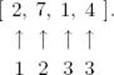
The deadline of each job has been listed under the job. Because job 4 is not scheduled by its deadline, the sequence is not feasible. By Lemma 4.3, the set is not feasible.

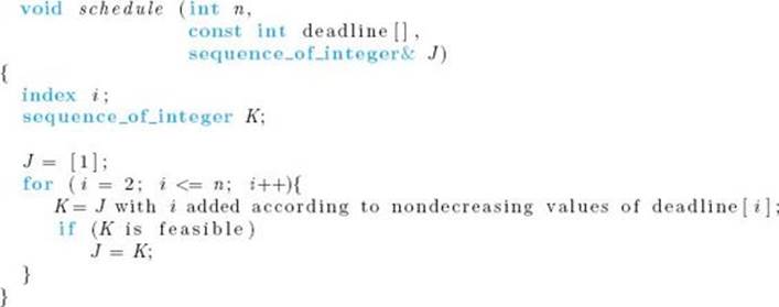
The algorithm follows. It is assumed that the jobs have already been sorted by profit in nonincreasing order, before being passed to the algorithm. Because the profits are needed only to sort the jobs, they are not listed as parameters of the algorithm.

Algorithm 4.4

Scheduling with Deadlines

Problem: Determine the schedule with maximum total profit given that each job has a profit that will be obtained only if the job is scheduled by its deadline.

Inputs: n, the number of jobs, and array of integers deadline, indexed from 1 to n, where deadline[i] is the deadline for the ith job. The array has been sorted in nonincreasing order according to the profits associated with the jobs.

Outputs: an optimal sequence J for the jobs.

Before analyzing this algorithm, let’s apply it.

Example 4.6

Suppose we have the jobs in Example 4.4. Recall that they had the following deadlines:

Algorithm 4.4 does the following:

1. J is set to [1].

2. K is set to [2, 1] and is determined to be feasible.
J is set to [2, 1] because K is feasible.

3. K is set to [2, 3, 1] and is rejected because it is not feasible.

4. K is set to [2, 1, 4] and is determined to be feasible.
J is set to [2, 1, 4] because K is feasible.

5. K is set to [2, 5, 1, 4] and is rejected because it is not feasible.

6. K is set to [2, 1, 6, 4] and is rejected because it is not feasible.

7. K is set to [2, 7, 1,4] and is rejected because it is not feasible.

The final value of J is [2, 1, 4].

Analysis of Algorithm 4.4

Worst-Case Time Complexity (Scheduling with Deadlines)

Basic operation: We need to do comparisons to sort the jobs, we need to do more comparisons when we set K equal to J with job i added, and we need to do comparisons to check if K is feasible. Therefore, a comparison instruction is the basic operation.

Input size: n, the number of jobs.

It takes a time of Θ(n lg n) to sort the jobs before passing them to the procedure. In each iteration of the for-i loop, we need to do at most i − 1 comparisons to add the ith job to K, and at most i comparisons to check if K is feasible. Therefore, the worst case is

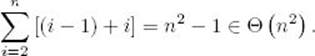
The first equality is obtained in Example A.1 in Appendix. Because this time dominates the sorting time,

Finally, we prove that the algorithm always gives an optimal solution.

Theorem 4.4

Algorithm 4.4 always produces an optimal set of jobs.

Proof: The proof is by induction on the number of jobs n.

Induction base: Clearly, the theorem holds if there is one job.

Induction hypothesis: Suppose the set of jobs that our algorithm obtains from the first n jobs is optimal for the first n jobs.

Induction step: We need to show that the set of jobs our algorithm obtains from the first n+1 jobs is optimal for the first n+1 jobs. To that end, let A be the set of jobs that our algorithm obtains from the first n+1 jobs and let B be an optimal set of jobs obtained from the first n + 1 jobs. Furthermore, let job(k) be the kth job in our sorted list of jobs.

There are two cases:

Case 1. B does not include job (n + 1).

In this case B is a set of jobs obtained from the first n jobs. However, by the induction hypothesis, A includes an optimal set of jobs obtained from the first n jobs. Therefore, the total profit of the jobs in B can be no greater than the total profit of the jobs in A, and A must be optimal.

Case 2. B includes job (n + 1).

Suppose A includes job (n + 1). Then

where B′ is a set obtained from the first n jobs and A′ is the set our algorithm obtains from the first n jobs. By the induction hypothesis, A′ is optimal for the first n jobs. Therefore,

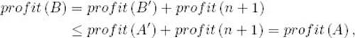
where profit (n + 1) is the profit of job (n + 1) and profit (A) is the total profit of the jobs in A. Since B is optimal for the first n + 1 jobs, we can conclude that A is also.

Suppose A does not include job (n + 1). Consider the time slot occupied by job (n + 1) in B. If that slot was available when our algorithm considered job (n + 1), it would schedule that job. Therefore, that time slot must be given to some job, say job (i₁), in A. If job (i₁) is in B, then whatever slot it occupies in B must be occupied by some job, say job (i₂), in A because otherwise our algorithm could have put job (i₁) in that slot and job (n + 1) in job (i₁)’s slot. Clearly, job (i₂) is not equal to job (i₁) or job (n + 1). If job (i₂) is in B, then whatever time slot it occupies in B must be occupied by some job, say job (i₃), in A because otherwise our algorithm could have put job (i₂) in that slot, job (i₁) in job (i₂)’s slot, and job (n + 1) in job (i₁)’s slot. Clearly, job (i₃) is not equal to job (i₂), job (i₁), or job (n + 1). We can repeat this argument indefinitely. Since the schedules are finite, we must therefore eventually arrive at a job, say job (i_k), which is in A and not in B. Otherwise, A ⊆ B, which means our algorithm could have scheduled job (n + 1) with the jobs in A. We can modify B by placing job (i₁) in job (n + 1)’s slot, job (i₂) in job (i₁)’s slot, …, and job (i_k) in job (i_k−1)’s slot. We have effectively replaced job (n + 1) by job (i_k) in B. Because the jobs are sorted in nondecreasing order, job (i_k)’s profit is at least as great as job (n + 1)’s profit. So we have a set of jobs that has a total profit at least as great as the total profit of the jobs in B. However, this set is obtained from the first njobs. Therefore, by the induction hypothesis, its total profit can be no greater than the total profit of the jobs in A, which means A is optimal.

Using Disjoint Set Data Structure III, which is presented in Appendix C, it is possible to create a Θ(n lg m) version of procedure schedule (in Algorithm 4.4), where m is the minimum of n and the largest of the deadlines for the n jobs. Because the time to sort is still in Θ(n lg n), the entire algorithm is Θ(n lg n). This modification will be discussed in the exercises.

4.4 Huffman Code

Even though the capacity of secondary storage devices keeps getting larger and their cost keeps getting smaller, the devices continue to fill up due to increased storage demands. Given a data file, it would therefore be desirable to find a way to store the file as efficiently as possible. The problem ofdata compression is to find an efficient method for encoding a data file. Next, we discuss the encoding method, called Huffman code, and a greedy algorithm for finding a Huffman encoding for a given file.

A common way to represent a file is to use a binary code. In such a code, each character is represented by a unique binary string, called the codeword. A fixed-length binary code represents each character using the same number of bits. For example, suppose our character set is {a, b, c}. Then we could use 2 bits to code each character, since this gives us four possible codewords and we need only three. We could code as follows:

Given this code, if our file is

our encoding is

We can obtain a more efficient coding using a variable-length binary code. Such a code can represent different characters using different numbers of bits. In the current example, we can code one of the characters as 0. Since ‘b’ occurs most frequently, it would be most efficient to code ‘b’ using this codeword. However, then ‘a’ could not be coded as ‘00’ because we would not be able to distinguish one ‘a’ from two ‘b’s. Furthermore, we would not want to code ‘a’ as ‘01’ because when we encountered a 0, we could not determine if it represented a ‘b’ or the beginning of an ‘a’ without looking beyond the current digit. So we could code as follows:

Given this code, File 4.1 would be encoded as

With this encoding it takes only 13 bits to represent the file, whereas the previous one took 18 bits. It is not hard to see that this encoding is optimal given that it is the minimum number of bits necessary to represent the file with a binary character code.

Given a file, the Optimal Binary Code problem is to find a binary character code for the characters in the file, which represents the file in the least number of bits. First we discuss prefix codes, and then we develop Huffman’s algorithm for solving this problem.

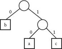
Figure 4.9 Binary tree corresponding to Code 4.2.

• 4.4.1 Prefix Codes

One particular type of variable-length code is a prefix code. In a prefix code no codeword for one character constitutes the beginning of the codeword for another character. For example, if 01 is the code word for ‘a’, then 011 could not be the codeword for ‘b’. Code 4.2 is an example of a prefix code. A fixed-length code is also a prefix code. Every prefix code can be represented by a binary tree whose leaves are the characters that are to be encoded. The binary tree corresponding to Code 4.2 appears in Figure 4.9. The advantage of a prefix code is that we need not look ahead when parsing the file. This is readily apparent from the tree representation of the code. To parse, we start at the first bit on the left in the file and the root of the tree. We sequence through the bits, and go left or right down the tree depending on whether a 0 or 1 is encountered. When we reach a leaf, we obtain the character at that leaf; then we return to the root and repeat the procedure starting with the next bit in sequence.

Example 4.7

Suppose our character set is {a, b, c, d, e, f} and each character appears in the file the number of times indicated in Table 4.1. That table also shows three different codes we could use to encode the file. Let’s compute the number of bits for each encoding:

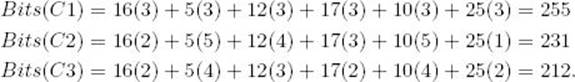
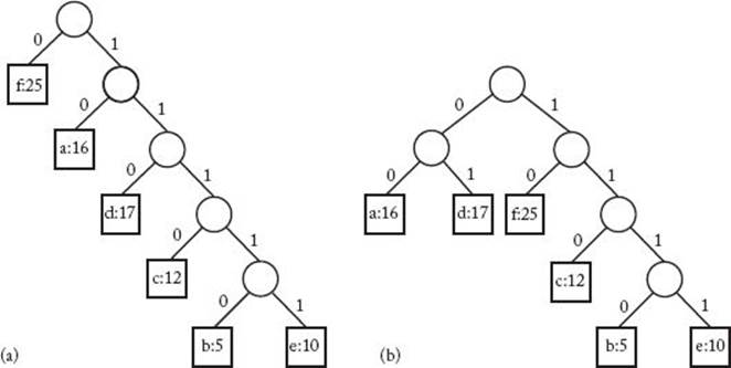
We see that Code C2 is an improvement on the fixed-length code C1, but C3 (Huffman) is even better than C2. As we shall see in the next subsection, C3 is optimal. The binary trees corresponding to Codes C2 and C3 appear in Figures 4.10(a) and (b), respectively. The frequency of each character appears with the character in the tree.

• Table 4.1 Three codes for the same file. C3 is optimal.

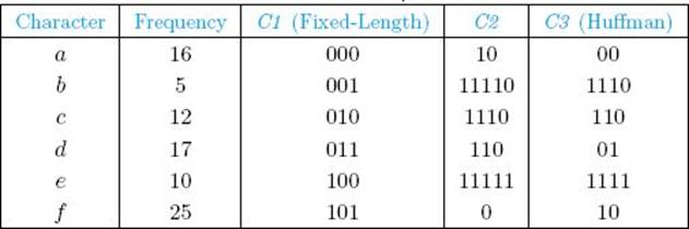
Figure 4.10 The binary character code for Code C2 in Example 4.7 appears in (a), while the one for Code C3 (Huffman) appears in (b).

As can be seen from the preceding example, the number of bits it takes to encode a file given the binary tree T corresponding to some code is given by

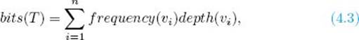
where {v₁, v₂, … v_n} is the set of characters in the file, frequency(v_i) is the number of times v_i occurs in the file, and depth(v_i) is the depth of v_i in T.

• 4.4.2 Huffman’s Algorithm

Huffman developed a greedy algorithm that produces an optimal binary character code by constructing a binary tree corresponding to an optimal code. A code produced by this algorithm is called a Huffman code. We present a high-level version of the algorithm. However, because it involvesconstructing a tree, we need to be more detailed than in our other high-level algorithms. In particular, we first have the following type declaration:

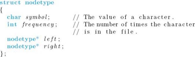
Furthermore, we need to use a priority queue. In a priority queue, the element with the highest priority is always removed next. In this case, the element with the highest priority is the character with the lowest frequency in the file. A priority queue can be implemented as a linked list, but more efficiently as a heap (See Section 7.6 for a discussion of heaps.) Huffman’s algorithm now follows.

n = number of characters in the file;

Arrange n pointers to nodetype records in a priority queue PQ as follows: For each pointer p in PQ

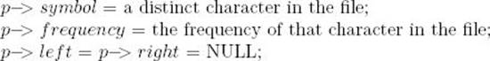
The priority is according to the value of frequency, with lower frequencies having higher priority.

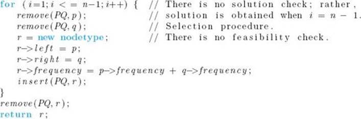
If a priority queue is implemented as a heap, it can be initialized in θ(n) time. Furthermore, each heap operation requires θ(lg n) time. Since there are n−1 passes through the for-i loop, the algorithm runs in θ(n lg n) time.

Next we show an example of applying the preceding algorithm.

Figure 4.11 Given the file whose frequencies are shown in Table 4.1, this shows the state of the subtrees, constructed by Huffman’s algorithm, after each pass through the for-i loop. The first tree is the state before the loop is entered.

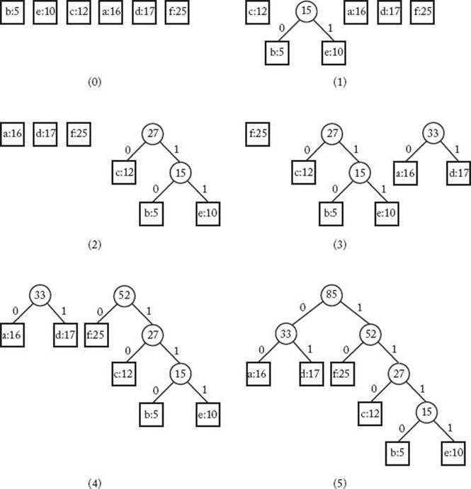
Example 4.8

Suppose our character set is {a, b, c, d, e, f} and each character appears in the file the number of times indicated in Table 4.1. Figure 4.11 shows the set of trees, constructed by the algorithm, after each pass through the for-i loop. The first set in the figure is before the loop is entered. The value stored at each node is the value of the frequency field in the node. Note that the final tree is the one in Figure 4.10(b).

Next we prove that the algorithm always produces an optimal binary character code. We start with a lemma:

Lemma 4.4

The binary tree corresponding to an optimal binary prefix code is full. That is, every nonleaf has two children.

Proof: The proof is left as an exercise.

Before proceeding, we need some terminology. Two nodes are called siblings in a tree if they have the same parent. A branch with root v in tree T is the subtree whose root is v. We now prove the optimality of Huffman’s algorithm.

Theorem 4.5

Huffman’s algorithm produces an optimal binary code.

Proof: The proof is by induction. Assuming the set of trees obtained in the ith step are branches in a binary tree corresponding to an optimal code, we show that the set of trees obtained in the (i + 1)st step are also branches in a binary tree corresponding to an optimal code. We conclude then that the binary tree produced in the (n − 1)st step corresponds to an optimal code.

Induction base: Clearly, the set of single nodes obtained in the 0 th step are branches in a binary tree corresponding to an optimal code.

Induction hypothesis: Assume the set of trees obtained in the ith step are branches in a binary tree corresponding to an optimal code. Let T be that tree.

Induction step: Let u and v be the roots of the trees combined in the (i + 1)st step of Huffman’s algorithm. If u and v are siblings in T, then we are done because the set of trees obtained in the (i + 1)st step of Huffman’s algorithm are branches in T.

Otherwise, without loss of generality, assume u is at a level in T at least as low as v. As before, let frequency(v) be the sum of the frequencies of the characters stored at the leaves of the branch rooted at v. Due to Lemma 4.4, u has some sibling w in T. Let S be the set of trees that exist after the ith step in Huffman’s algorithm. Clearly, the branch in T whose root is w is one of the trees in S or contains one of those trees as a subtree. In either case, since the tree whose root is v was chosen by Huffman’s algorithm in this step,

Furthermore, in T

We can create a new binary tree T′ by swapping the positions of the branches rooted at v and w in T. This is depicted in Figure 4.12. It is not hard to see from Equality 4.3 and the previous two inequalities that

Figure 4.12 The branches rooted at v and w are swapped.

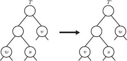
which means the code corresponding to T′ is optimal. Clearly, the set of trees obtained in the (i + 1)st step of Huffman’s algorithm are branches in T′.

4.5 The Greedy Approach versus Dynamic Programming: The Knapsack Problem

The greedy approach and dynamic programming are two ways to solve optimization problems. Often a problem can be solved using either approach. For example, the Single-Source Shortest Paths problem is solved using dynamic programming in Algorithm 3.3 and is solved using the greedy approach in Algorithm 4.3. However, the dynamic programming algorithm is overkill in that it produces the shortest paths from all sources. There is no way to modify the algorithm to produce more efficiently only shortest paths from a single source because the entire array D is needed regardless. Therefore, the dynamic programming approach yields a Θ(n³) algorithm for the problem, whereas the greedy approach yields a Θ(n²) algorithm. Often when the greedy approach solves a problem, the result is a simpler, more efficient algorithm.

On the other hand, it is usually more difficult to determine whether a greedy algorithm always produces an optimal solution. As the Change problem shows, not all greedy algorithms do. A proof is needed to show that a particular greedy algorithm always produces an optimal solution, whereas a counterexample is needed to show that it does not. Recall that in the case of dynamic programming we need only determine whether the principle of optimality applies.

To illuminate further the differences between the two approaches, we will present two very similar problems, the 0-1 Knapsack problem and the Fractional Knapsack problem. We will develop a greedy algorithm that successfully solves the Fractional Knapsack problem but fails in the case of the 0-1 Knapsack problem. Then we will successfully solve the 0-1 Knapsack problem using dynamic programming.

• 4.5.1 A Greedy Approach to the 0-1 Knapsack Problem

An example of this problem concerns a thief breaking into a jewelry store carrying a knapsack. The knapsack will break if the total weight of the items stolen exceeds some maximum weight W. Each item has a value and a weight. The thief’s dilemma is to maximize the total value of the items while not making the total weight exceed W. This problem is called the 0-1 Knapsack problem. It can be formalized as follows.

Suppose there are n items. Let

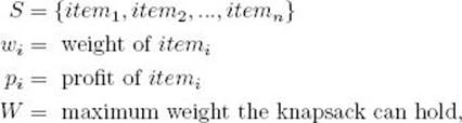
where w_i, p_i, and W are positive integers. Determine a subset A of S such that

The brute-force solution is to consider all subsets of the n items; discard those subsets whose total weight exceeds W; and, of those remaining, take one with maximum total profit. Example A.10 in Appendix A shows that there are 2ⁿ subsets of a set containing n items. Therefore, the brute-force algorithm is exponential-time.

An obvious greedy strategy is to steal the items with the largest profit first; that is, steal them in nonincreasing order according to profit. This strategy, however, would not work very well if the most profitable item had a large weight in comparison to its profit. For example, suppose we had three items, the first weighing 25 pounds and having a profit of $10, and the second and third each weighing 10 pounds and having a profit of $9. If the capacity W of the knapsack was 30 pounds, this greedy strategy would yield only a profit of $10, whereas the optimal solution is $18.

Another obvious greedy strategy is to steal the lightest items first. This strategy fails badly when the light items have small profits compared with their weights.

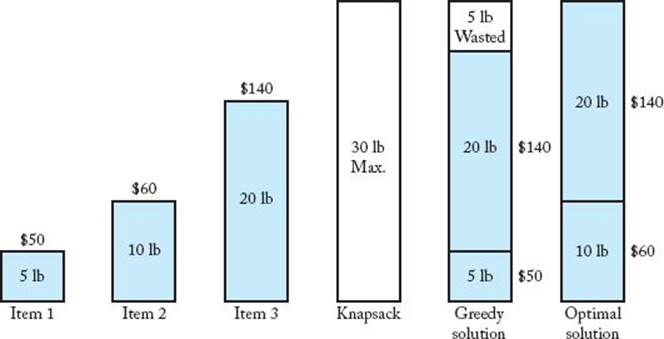
To avoid the pitfalls of the previous two greedy algorithms, a more sophisticated greedy strategy is to steal the items with the largest profit per unit weight first. That is, we order the items in nonincreasing order according to profit per unit weight, and select them in sequence. An item is put in the knapsack if its weight does not bring the total weight above W. This approach is illustrated in Figure 4.13. In that figure, the weight and profit for each item are listed by the item, and the value of W, which is 30, is listed in the knapsack. We have the following profits per unit weight:

Figure 4.13 A greedy solution and an optimal solution to the 0-1 Knapsack problem.

Ordering the items by profit per unit weight yields

As can be seen in the figure, this greedy approach chooses item₁ and item₃, resulting in a total profit of $190, whereas the optimal solution is to choose item₂ and item₃, resulting in a total profit of $200. The problem is that after item₁ and item₃ are chosen, there are 5 pounds of capacity left, but it is wasted because item₂ weighs 10 pounds. Even this more sophisticated greedy algorithm does not solve the 0-1 Knapsack problem.

• 4.5.2 A Greedy Approach to the Fractional Knapsack Problem

In the Fractional Knapsack problem, the thief does not have to steal all of an item, but rather can take any fraction of the item. We can think of the items in the 0-1 Knapsack problem as being gold or silver ingots and the items in the Fractional Knapsack problem as being bags of gold or silver dust. Suppose we have the items in Figure 4.13. If our greedy strategy is again to choose the items with the largest profit per unit weight first, all of item₁ and item₃ will be taken as before. However, we can use the 5 pounds of remaining capacity to take 5/10 of item₂. Our total profit is

Our greedy algorithm never wastes any capacity in the Fractional Knapsack problem as it does in the 0-1 Knapsack problem. As a result, it always yields an optimal solution. You are asked to prove this in the exercises.

• 4.5.3 A Dynamic Programming Approach to the 0-1 Knapsack Problem

If we can show that the principle of optimality applies, we can solve the 0-1 Knapsack problem using dynamic programming. To that end, let A be an optimal subset of the n items. There are two cases: either A contains item_n or it does not. If A does not contain item_n, A is equal to an optimal subset of the first n − 1 items. If A does contain item_n, the total profit of the items in A is equal to p_n plus the optimal profit obtained when the items can be chosen from the first n − 1 items under the restriction that the total weight cannot exceed W − w_n. Therefore, the principle of optimality applies.

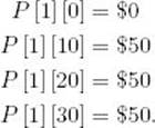
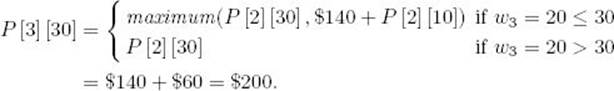
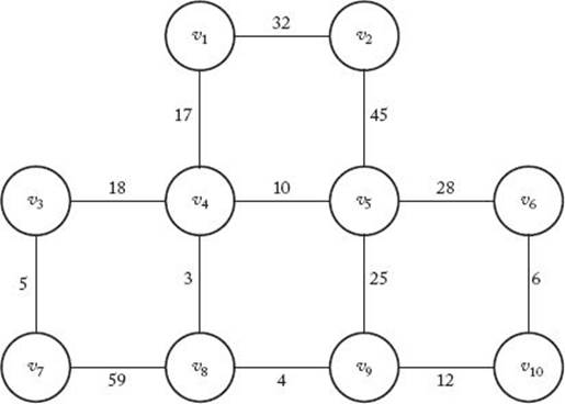
The result just obtained can be generalized as follows. If for i > 0 and w > 0, we let P [i][w] be the optimal profit obtained when choosing items only from the first i items under the restriction that the total weight cannot exceed w,

The maximum profit is equal to P [n] [W]. We can determine this value using a two-dimensional array P whose rows are indexed from 0 to n and whose columns are indexed from 0 to W. We compute the values in the rows of the array in sequence using the previous expression for P [i] [w]. The values of P [0] [w] and P [i] [0] are set to 0. You are asked to actually write the algorithm in the exercises. It is straightforward that the number of array entries computed is

• 4.5.4 A Refinement of the Dynamic Programming Algorithm for the 0-1 Knapsack Problem

The fact that the previous expression for the number of array entries computed is linear in n can mislead one into thinking that the algorithm is efficient for all instances containing n items. This is not the case. The other term in that expression is W, and there is no relationship between n and W. Therefore, for a given n, we can create instances with arbitrarily large running times by taking arbitrarily large values of W. For example, the number of entries computed is in Θ(n × n!) if W equals n!. If n = 20 and W = 20!, the algorithm will take thousands of years to run on a modern-day computer. When W is extremely large in comparison with n, this algorithm is worse than the brute-force algorithm that simply considers all subsets.

The algorithm can be improved so that the worst-case number of entries computed is in Θ(2ⁿ). With this improvement, it never performs worse than the brute-force algorithm and often performs much better. The improvement is based on the fact that it is not necessary to determine the entries in the ith row for every w between 1 and W. Rather, in the nth row we need only determine P [n] [W]. Therefore, the only entries needed in the (n − 1)st row are the ones needed to compute P [n] [W]. Because

the only entries needed in the (n − 1)st row are

We continue to work backward from n to determine which entries are needed. That is, after we determine which entries are needed in the ith row, we determine which entries are needed in the (i − 1)st row using the fact that

We stop when n = 1 or w ≤ 0. After determining the entries needed, we do the computations starting with the first row. The following example illustrates this method.

Example 4.9

Suppose we have the items in Figure 4.13 and W = 30. First we determine which entries are needed in each row.

Determine entries needed in row 3:

We need

Determine entries needed in row 2:

To compute P [3] [30], we need

Determine entries needed in row 1:

To compute P [2] [30], we need

To compute P [2] [10], we need

Next we do the computations.

Compute row 1:

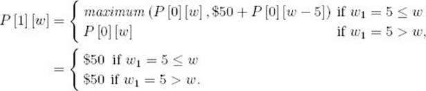
Therefore,

Compute row 2:

Compute row 3:

This version of the algorithm computes only seven entries, whereas the original version would have computed (3) (30) = 90 entries.

Let’s determine how efficient this version is in the worst case. Notice that we compute at most 2ⁱ entries in the (n − i)th row. Therefore, at most the total number of entries computed is

This equality is obtained in Example A.3 in Appendix A. It is left as an exercise to show that the following is an instance for which about 2ⁿ entries are computed (the profits can have any values):

Combining these two results, we can conclude that the worst-case number of entries computed is in

The previous bound is in terms of only n. Let’s also obtain a bound in terms of n and W combined. We know that the number of entries computed is in O (nW), but perhaps this version avoids ever reaching this bound. This is not the case. In the exercises you will show that if n = W + 1 and w_i = 1 for all i, then the total number of entries computed is about

The first equality is obtained in Example A.1 in Appendix A, and the second derives from the fact that n = W +1 in this instance. Therefore, this bound is reached for arbitrarily large values of n and W, which means the worst-case number of entries computed is in

Combining our two results, the worst-case number of entries computed is in

We do not need to create the entire array to implement the algorithm. Instead, we can store just the entries that are needed. The entire array exists only implicitly. If the algorithm is implemented in this manner, the worst-case memory usage has these same bounds.

We could write a divide-and-conquer algorithm using the expression for P [i] [w] that was used to develop the dynamic programming algorithm. For this algorithm the worst-case number of entries computed is also in Θ(2ⁿ). The main advantage of the dynamic programming algorithm is theadditional bound in terms of nW. The divide-and-conquer algorithm does not have this bound. Indeed, this bound is obtained because of the fundamental difference between dynamic programming and divide-and-conquer. That is, dynamic programming does not process the same instance more than once. The bound in terms of nW is very significant when W is not large in comparison with n.

As is the case for the Traveling Salesperson problem, no one has ever found an algorithm for the 0-1 Knapsack problem whose worst-case time complexity is better than exponential, yet no one has proven that such an algorithm is not possible. Such problems are the focus of Chapter 9.

EXERCISES

Sections 4.1

1. Show that the greedy approach always finds an optimal solution for the Change problem when the coins are in the denominations D⁰, D¹, D², … , Dⁱ for some integers i > 0 and D > 0.

2. Use Prim’s algorithm (Algorithm 4.1) to find a minimum spanning tree for the following graph. Show the actions step by step.

3. Consider the following array:

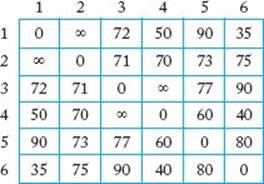
(a) Starting with vertex v₄, trace through Prim’s algorithm to find a minimum spanning tree for the graph represented by the array shown here.

(b) Show the set of edges that comprise the minimum spanning tree.

(c) What is the cost of the minimum spanning tree?

4. Draw a graph that has more than one minimum spanning tree.

5. Implement Prim’s algorithm (Algorithm 4.1) on your system, and study its performance using different graphs.

6. Modify Prim’s algorithm (Algorithm 4.1) to check if an undirected, weighted graph is connected. Analyze your algorithm and show the results using order notation.

7. Use Kruskal’s algorithm (Algorithm 4.2) to find a minimum spanning tree for the graph in Exercise 2. Show the actions step by step.

8. Implement Kruskal’s algorithm (Algorithm 4.2) on your system, and study its performance using different graphs.

9. Do you think it is possible for a minimum spanning tree to have a cycle? Justify your answer.

10. Assume that in a network of computers any two computers can be linked. Given a cost estimate for each possible link, should Algorithm 4.1 (Prim’s algorithm) or Algorithm 4.2 (Kruskal’s algorithm) be used? Justify your answer.

11. Apply Lemma 4.2 to complete the proof of Theorem 4.2.

Sections 4.2

12. Use Dijkstra’s algorithm (Algorithm 4.3) to find the shortest path from vertex v₅ to all the other vertices for the graph represented by the array in Exercise 3. Show the actions step by step.

13. Use Dijkstra’s algorithm (Algorithm 4.3) to find the shortest paths from the vertex v₄ to all the other vertices of the graph in Exercise 2. Show the actions step by step. Assume that each undirected edge represents two directed edges with the same weight.

14. Implement Dijkstra’s algorithm (Algorithm 4.3) on your system, and study its performance using different graphs.

15. Modify Dijkstra’s algorithm (Algorithm 4.3) so that it computes the lengths of the shortest paths. Analyze the modified algorithm and show the results using order notation.

16. Modify Dijkstra’s algorithm (Algorithm 4.3) so that it checks if a directed graph has a cycle. Analyze your algorithm and show the results using order notation.

17. Can Dijkstra’s algorithm (Algorithm 4.3) be used to find the shortest paths in a graph with some negative weights? Justify your answer.

18. Use induction to prove the correctness of Dijkstra’s algorithm (Algorithm 4.3).

Sections 4.3

19. Consider the following jobs and service times. Use the algorithm in Section 4.3.1 to minimize the total amount of time spent in the system.

20. Implement the algorithm in Section 4.3.1 on your system, and run it on the instance in Exercise 17.

21. Write an algorithm for the generalization of the Single-Server Scheduling problem to the Multiple-Server Scheduling problem in Section 4.3.1. Analyze your algorithm and show the results using order notation.

22. Consider the following jobs, deadlines, and profits. Use the Scheduling with Deadlines algorithm (Algorithm 4.4) to maximize the total profit.

23. Consider procedure schedule in the Scheduling with Deadlines algorithm (Algorithm 4.4). Let d be the maximum of the deadlines for n jobs. Modify the procedure so that it adds a job as late as possible to the schedule being built, but no later than its deadline. Do this by initializing d + 1 disjoint sets, containing the integers 0, 1, … , d. Let small (S) be the smallest member of set S. When a job is scheduled, find the set S containing the minimum of its deadline and n. If small (S) = 0, reject the job. Otherwise, schedule it at time small (S), and merge S with the set containing small(S) − 1. Assuming we use Disjoint Set Data Structure III in Appendix C, show that this version is θ (n lg m), where m is the minimum of d and n.

24. Implement the algorithm developed in Exercise 21.

25. Suppose we minimize the average time to store n files of lengths l₁, l₂, … , l_n on a tape. If the probability of requesting file k is given by p_k, the expected access time to load these n files in the order k₁, k₂, … , k_n is given by the formula

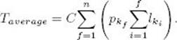
The constant C represents parameters such as the speed of the drive and the recording density.

(a) In what order should a greedy approach store these files to guarantee minimum average access time?

(b) Write the algorithm that stores the files, analyze your algorithm, and show the results using order notation.

Sections 4.4

26. Use Huffman’s algorithm to construct an optimal binary prefix code for the letters in the following table.

27. Use Huffman’s algorithm to construct an optimal binary prefix code for the letters in the following table.

28. Decode each bit string using the binary code in Exercise 24.

(a) 01100010101010

(b) 1000100001010

(c) 11100100111101

(d) 1000010011100

29. Encode each word using the binary code in Exercise 25.

(a) rise

(b) exit

(c) text

(d) exercise

30. A code for a, b, c, d, e is given by a:00, b:01, c:101, d:x 10, e:yz 1, where x, y, z are in 0,1. Determine x, y and z so that the given code is a prefix code.

31. Implement Huffman’s algorithm, and run it on the problem instances of Exercise 24 and 25.

32. Show that a binary tree corresponding to an optimal binary prefix code must be full. A full binary tree is a binary tree such that every node is either a leaf or it has two children.

33. Prove that for an optimal binary prefix code, if the characters are ordered so that their frequencies are nonincreasing, then their codeword lengths are nondecreasing.

34. Given the binary tree corresponding to a binary prefix code, write an algorithm that determines the codewords for all the characters. Determine the time complexity of your algorithm.

Sections 4.5

35. Write the dynamic programming algorithm for the 0-1 Knapsack problem.

36. Use a greedy approach to construct an optimal binary search tree by considering the most probable key, Key_k, for the root, and constructing the left and right subtrees for Key₁, Key₂, … , Key_k−1 and Key_k+1, Key_k+2, … , Key_n recursively in the same way.

(a) Assuming the keys are already sorted, what is the worst-case time complexity of this approach? Justify your answer.

(b) Use an example to show that this greedy approach does not always find an optimal binary search tree.

37. Suppose we assign n persons to n jobs. Let C_ij be the cost of assigning the ith person to the jth job. Use a greedy approach to write an algorithm that finds an assignment that minimizes the total cost of assigning all n persons to all n jobs. Analyze your algorithm and show the results using order notation.

38. Use the dynamic programming approach to write an algorithm for the problem of Exercise 26. Analyze your algorithm and show the results using order notation.

39. Use a greedy approach to write an algorithm that minimizes the number of record moves in the problem of merging n files. Use a two-way merge pattern. (Two files are merged during each merge step.) Analyze your algorithm, and show the results using order notation.

40. Use the dynamic programming approach to write an algorithm for Exercise

28. Analyze your algorithm and show the results using order notation.

41. Prove that the greedy approach to the Fractional Knapsack problem yields an optimal solution.

42 Show that the worst-case number of entries computed by the refined dynamic programming algorithm for the 0-1 Knapsack problem is in Ω(2ⁿ). Do this by considering the instance in which W = 2ⁿ −2 and w_i = 2ⁱ⁻¹ for 1 ≤ i ≤ n.

43. Show that in the refined dynamic programming algorithm for the 0-1 Knapsack problem, the total number of entries computed is about (W + 1) × (n + 1) /2, when n = W + 1 and w_i = 1 for all i.

Additional Exercises

44. Show with a counterexample that the greedy approach does not always yield an optimal solution for the Change problem when the coins are U.S. coins and we do not have at least one of each type of coin.

45. Prove that a complete graph (a graph in which there is an edge between every pair of vertices) has nⁿ⁻² spanning trees. Here n is the number of vertices in the graph.

46. Use a greedy approach to write an algorithm for the Traveling Salesperson problem. Show that your algorithm does not always find a minimum-length tour.

47. Prove that the algorithm for the Multiple-Server Scheduling problem of Exercise 19 always finds an optimal schedule.

48. Without constructing a Huffman tree, generate Huffman code for a given set of characters.

49. Generalize Huffman’s algorithm to ternary code words and prove that it yields optimal ternary codes.

50. Show that if the characters are sorted according to their frequencies, then the Huffman tree can be constructed in linear time.