Foundations of Algorithms (2015)
Chapter 6 Branch-and-Bound
We’ve provided our thief with two algorithms for the 0-1 Knapsack problem: the dynamic programming algorithm in Section 4.5 and the backtracking algorithm in Section 5.7. Because both these algorithms are exponential-time in the worst case, they could both take many years to solve our thief’s particular instance. In this chapter, we provide our thief with yet another approach, called branch-and-bound. As we shall see, the branch-and-bound algorithm developed here is an improvement on the backtracking algorithm. Therefore, even if the other two algorithms fail to solve our thief’s instance efficiently, the branch-and-bound algorithm might do so.
The branch-and-bound design strategy is very similar to backtracking in that a state space tree is used to solve a problem. The differences are that the branch-and-bound method (1) does not limit us to any particular way of traversing the tree and (2) is used only for optimization problems. A branch-and-bound algorithm computes a number (bound) at a node to determine whether the node is promising. The number is a bound on the value of the solution that could be obtained by expanding beyond the node. If that bound is no better than the value of the best solution found so far, the node is nonpromising. Otherwise, it is promising. Because the optimal value is a minimum in some problems and a maximum in others, by “better” we mean smaller or larger, depending on the problem. As is the case for backtracking algorithms, branch-and-bound algorithms are ordinarily exponential-time (or worse) in the worst case. However, they can be very efficient for many large instances.
The backtracking algorithm for the 0-1 Knapsack problem in Section 5.7 is actually a branch-and-bound algorithm. In that algorithm, the promising function returns false if the value of bound is not greater than the current value of maxprofit. A backtracking algorithm, however, does not exploit the real advantage of using branch-and-bound. Besides using the bound to determine whether a node is promising, we can compare the bounds of promising nodes and visit the children of the one with the best bound.
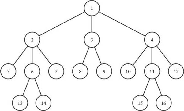
Figure 6.1 A breadth-first search of a tree. The nodes are numbered in the order in which they are visited. The children of a node are visited from left to right.
In this way we often can arrive at an optimal solution faster than we would by methodically visiting the nodes in some predetermined order (such as a depth-first search). This approach is called best-first search with branch-and-bound pruning. The implementation of the approach is a simple modification of another methodical approach called breadth-first search with branch-and-bound pruning. Therefore, even though this latter technique has no advantage over depth-first search, in Section 6.1 we will first solve the 0-1 Knapsack problem using a breadth-first search. This will enable us to more easily explain best-first search and use it to solve the 0-1 Knapsack problem. Sections 6.2 and 6.3 apply the best-first search approach to two more problems.
Before proceeding, we review breadth-first search. In the case of a tree, a breadth-first search consists of visiting the root first, followed by all nodes at level 1, followed by all nodes at level 2, and so on. Figure 6.1 shows a breadth-first search of a tree in which we proceed from left to right. The nodes are numbered according to the order in which they are visited.
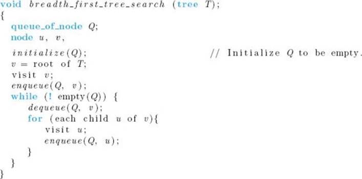
Unlike depth-first search, there is no simple recursive algorithm for breadth-first search. However, we can implement it using a queue. The algorithm that follows does this. The algorithm is written specifically for trees because presently we are interested only in trees. We insert an item at the end of the queue with a procedure called enqueue, and we remove an item from the front with a procedure called dequeue.
If you are not convinced that this procedure produces a breadth-first search, you should walk through an application of this algorithm to the tree in Figure 6.1. In that tree, as mentioned previously, a node’s children are visited from left to right.
6.1 Illustrating Branch-and-Bound with the 0-1 Knapsack problem
We show how to use the branch-and-bound design strategy by applying it to the 0-1 Knapsack problem. First we discuss a simple version called breadth-first search with branch-and-bound pruning. After that, we show an improvement on the simple version called best-first search with branch-and-bound pruning.
• 6.1.1 Breadth-First Search with Branch-and-Bound Pruning
Let’s demonstrate this approach with an example.
Example 6.1
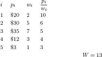
Suppose we have the instance of the 0-1 Knapsack problem presented in Exercise 5.6. That is, n = 4, W = 16, and we have the following:
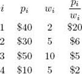
As in Example 5.6, the items have already been ordered according to pi/wi. Using breadth-first search with branch-and-bound pruning, we proceed exactly as we did using backtracking in Example 5.6, except that we do a breadth-first search instead of a depth-first search. That is, we let weightand profit be the total weight and total profit of the items that have been included up to a node. To determine whether the node is promising, we initialize totweight and bound to weight and profit, respectively, and then greedily grab items, adding their weights and profits to totweight and bound, until we reach an item whose weight would bring totweight above W . We grab the fraction of that item allowed by the available weight, and add the profit of that fraction to bound. In this way, bound becomes an upper bound on the amount of profit we could obtain by expanding beyond the node. If the node is at level i, and the node at level k is the one whose weight would bring the weight above W , then
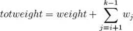
and

A node is nonpromising if this bound is less than or equal to maxprofit, which is the value of the best solution found up to that point. Recall that a node is also nonpromising if
![]()
The pruned state space tree produced using a breadth-first search on the instance in this example, with branches pruned using the bounds indicated above, is shown in Figure 6.2. The values of profit, weight, and bound are specified from top to bottom at each node. The node shaded in color is where the maximum profit is found. The nodes are labeled according to their levels and positions from the left in the tree.
Because the steps are so similar to those in Example 5.6, we will not walk through them. We mention only a few important points. We refer to a node by its level and position from the left in the tree. First, notice that nodes (3, 1) and (4, 3) have bounds of $0. A branch-and-bound algorithm decides whether to expand beyond a node by checking whether its bound is better than the value of the best solution found so far. Therefore, when a node is nonpromising because its weight is not less than W, we set its bound to $0. In this way, we ensure that its bound cannot be better than the value of the best solution found so far. Second, recall that when backtracking (depth-first search) was used on this instance, node (1, 2) was found to be nonpromising and we did not expand beyond the node.
Figure 6.2 The pruned state space tree produced using breadth-first search with branch-and-bound pruning in Example 6.1. Stored at each node from top to bottom are the total profit of the items stolen up to that node, their total weight, and the bound on the total profit that could be obtained by expanding beyond the node. The node shaded in color is the one at which an optimal solution is found.
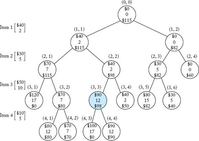
However, in the case of a breadth-first search, this node is the third node visited. At the time it is visited, the value of maxprofit is only $40. Because its bound $82 exceeds maxprofit at this point, we expand beyond the node. Last of all, in a simple breadth-first search with branch-and-bound pruning, the decision of whether or not to visit a node’s children is made at the time the node is visited. That is, if the branches to the children are pruned, they are pruned when the node is visited. Therefore, when we visit node (2, 3), we decide to visit its children because the value of maxprofit at that time is only $70, whereas the bound for the node is $82. Unlike a depth-first search, in a breadth-first search the value of maxprofit can change by the time we actually visit the children. In this case, maxprofit has a value of $90 by the time we visit the children of node (2, 3). We then waste our time checking these children. We avoid this in our best-first search, which is described in the next subsection.
Now that we have illustrated the technique, we present a general algorithm for breadth-first search with branch-and-bound pruning. Although we refer to the state space tree T as the input to this general-purpose algorithm, in actual applications the state space tree exists only implicitly. The parameters of the problem are the actual inputs to the algorithm and determine the state space tree T .
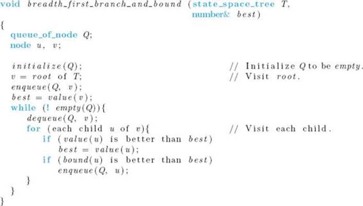
This algorithm is a modification of the breadth-first search algorithm presented at the beginning of this chapter. In this algorithm, however, we expand beyond a node (visit a node’s children) only if its bound is better than the value of the current best solution. The value of the current best solution (the variable best) is initialized to the value of the solution at the root. In some applications, there is no solution at the root because we must be at a leaf in the state space tree to have a solution. In such cases, we initialize best to a value that is worse than that of any solution. The functions bound andvalue are different in each application of breadth_first_branch_and_bound. As we shall see, we often do not actually write a function value. We simply compute the value directly.
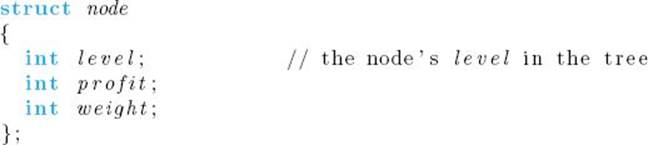
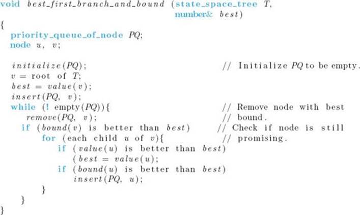
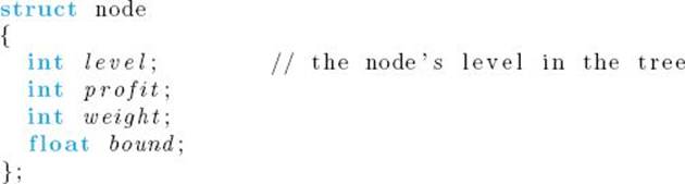
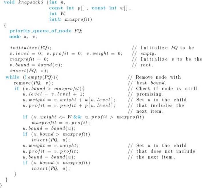
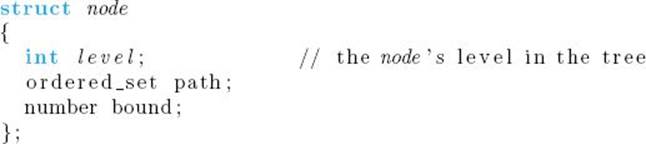
Next we present a specific algorithm for the 0-1 Knapsack problem. Because we do not have the benefit of recursion (which means we do not have new variables being created at each recursive call), we must store all the information pertinent to a node at that node. Therefore, the nodes in our algorithm will be of the following type:
![]() Algorithm 6.1
Algorithm 6.1
The Breadth-First Search with Branch-and-Bound Pruning Algorithm for the 0-1 Knapsack problem
Problem: Let n items be given, where each item has a weight and a profit. The weights and profits are positive integers. Furthermore, let a positive integer W be given. Determine a set of items with maximum total profit, under the constraint that the sum of their weights cannot exceed W .
Inputs: positive integers n and W , arrays of positive integers w and p, each indexed from 1 to n, and each of which is sorted in nonincreasing order according to the values of p [i] /w [i].
Outputs: an integer maxprofit that is the sum of the profits in an optimal set.
We do not need to check whether u.profit exceeds maxprofit when the current item is not included because, in this case, u.profit is the profit associated with u’s parent, which means that it cannot exceed maxprofit. We do not need to store the bound at a node (as depicted in Figure 6.2) because we have no need to refer to the bound after we compare it with maxprofit.
Function bound is essentially the same as function promising in Algorithm 5.7. The difference is that we have written bound according to guidelines for creating branch-and-bound algorithms, and therefore bound returns an integer. Function promising returns a boolean value because it was written according to backtracking guidelines. In our branch-and-bound algorithm, the comparison with maxprofit is done in the calling procedure. There is no need to check for the condition i = n in function bound because in this case the value returned by bound is less than or equal to maxprofit, which means that the node is not put in the queue.
Algorithm 6.1 does not produce an optimal set of items; it only determines the sum of the profits in an optimal set. The algorithm can be modified to produce an optimal set as follows. At each node we also store a variable items, which is the set of items that have been included up to the node, and we maintain a variable bestitems, which is the current best set of items. When maxprofit is set equal to u.profit, we also set bestitems equal to u.items.
• 6.1.2 Best-First Search with Branch-and-Bound Pruning
In general, the breadth-first search strategy has no advantage over a depth-first search (backtracking). However, we can improve our search by using our bound to do more than just determine whether a node is promising. After visiting all the children of a given node, we can look at all the promising, unexpanded nodes and expand beyond the one with the best bound. Recall that a node is promising if its bound is better than the value of the best solution found so far. In this way, we often arrive at an optimal solution more quickly than if we simply proceeded blindly in a predetermined order. The example that follows illustrates this method.
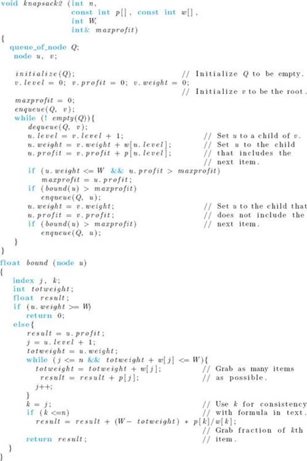
Example 6.2
Suppose we have the instance of the 0-1 Knapsack problem in Example 6.1. A best-first search produces the pruned state space tree in Figure 6.3. The values of profit, weight, and bound are again specified from top to bottom at each node in the tree. The node shaded in color is where the maximum profit is found. Next we show the steps that produced this tree. We again refer to a node by its level and its position from the left in the tree. Values and bounds are computed in the same way as in Examples 5.6 and 6.1. We do not show the computations while walking through the steps. Furthermore, we only mention when a node is found to be nonpromising; we do not mention when it is found to be promising.
The steps are as follows:
1. Visit node (0, 0) (the root).
(a) Set its profit and weight to $0 and 0.
(b) Compute its bound to be $115. (See Example 5.6 for the computation.)
(c) Set maxprofit to 0.
2. Visit node (1, 1).
(a) Compute its profit and weight to be $40 and 2.
(b) Because its weight 2 is less than or equal to 16, the value of W, and its profit $40 is greater than $0, the value of maxprofit, set maxprofit to $40.
(c) Compute its bound to be $115.
3. Visit node (1, 2).
(a) Compute its profit and weight to be $0 and 0.
(b) Compute its bound to be $82.
Figure 6.3 The pruned state space tree produced using best-first search with branch-and-bound pruning in Example 6.2. Stored at each node from top to bottom are the total profit of the items stolen up to the node, their total weight, and the bound on the total profit that could be obtained by expanding beyond the node. The node shaded in color is the one at which an optimal solution is found.
4. Determine promising, unexpanded node with the greatest bound.
(a) Because node (1, 1) has a bound of $115 and node (1, 2) has a bound of $82, node (1, 1) is the promising, unexpanded node with the greatest bound. We visit its children next.
5. Visit node (2, 1).
(a) Compute its profit and weight to be $70 and 7.
(b) Because its weight 7 is less than or equal to 16, the value of W , and its profit $70 is greater than $40, the value of maxprofit, set maxprofit to $70.
(c) Compute its bound to be $115.
6. Visit node (2, 2).
(a) Compute its profit and weight to be $40 and 2.
(b) Compute its bound to be $98.
7. Determine promising, unexpanded node with the greatest bound.
(a) That node is node (2, 1). We visit its children next.
8. Visit node (3, 1).
(a) Compute its profit and weight to be $120 and 17.
(b) Determine that it is nonpromising because its weight 17 is greater than or equal to 16, the value of W. We make it nonpromising by setting its bound to $0.
9. Visit node (3, 2).
(a) Compute its profit and weight to be $70 and 7.
(b) Compute its bound to be $80.
10. Determine promising, unexpanded node with the greatest bound.
(a) That node is node (2, 2). We visit its children next.
11. Visit node (3, 3).
(a) Compute its profit and weight to be $90 and 12.
(b) Because its weight 12 is less than or equal to 16, the value of W, and its profit $90 is greater than $70, the value of maxprofit, set maxprofit to $90.
(c) At this point, nodes (1, 2) and (3, 2) become nonpromising because their bounds, $82 and $80 respectively, are less than or equal to $90, the new value of maxprofit.
(d) Compute its bound to be $98.
12. Visit node (3, 4).
(a) Compute its profit and weight to be $40 and 2.
(b) Compute its bound to be $50.
(c) Determine that it is nonpromising because its bound $50 is less than or equal to $90, the value of maxprofit.
13. Determine promising, unexpanded node with the greatest bound.
(a) The only unexpanded, promising node is node (3, 3). We visit its children next.
14. Visit node (4, 1).
(a) Compute its profit and weight to be $100 and 17.
(b) Determine that it is nonpromising because its weight 17 is greater than or equal to 16, the value of W . We set its bound to $0.
15. Visit node (4, 2).
(a) Compute its profit and weight to be $90 and 12.
(b) Compute its bound to be $90.
(c) Determine that it is nonpromising because its bound $90 is less than or equal to $90, the value of maxprofit. Leaves in the state space tree are automatically nonpromising because their bounds cannot exceed maxprofit.
Because there are now no promising, unexpanded nodes, we are done.
Using best-first search, we have checked only 11 nodes, which is 6 less than the number checked using breadth-first search (Figure 6.2) and 2 less than the number checked using depth-first search (see Figure 5.14). A savings of 2 is not very impressive; however, in a large state space tree, the savings can be very significant when the best-first search quickly hones in on an optimal solution. It must be stressed, however, that there is no guarantee that the node that appears to be best will actually lead to an optimal solution. In Example 6.2, node (2, 1) appears to be better than node (2, 2), but node (2, 2) leads to the optimal solution. In general, best-first search can still end up creating most or all of the state space tree for some instances.
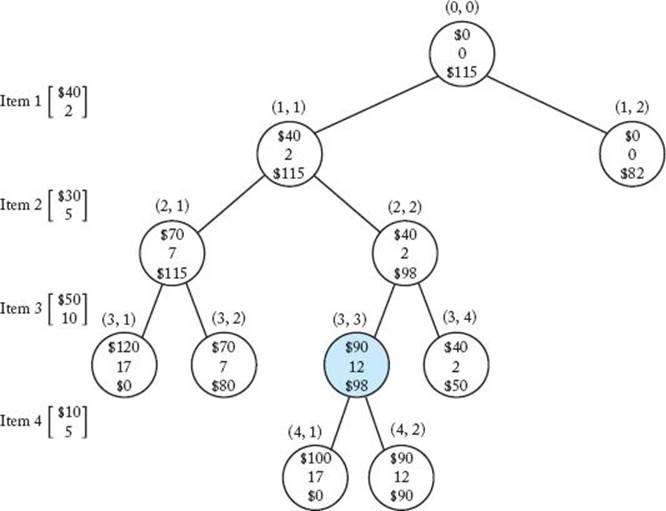
The implementation of best-first search consists of a simple modification to breadth-first search. Instead of using a queue, we use a priority queue. Recall that priority queues were discussed in Section 4.4.2. A general algorithm for the best-first search algorithm follows. Again, the tree T exists only implicitly. In the algorithm, insert (PQ, v) is a procedure that adds v to the priority queue PQ, whereas remove (PQ, v) is a procedure that removes the node with the best bound and assigns its value to v.
Besides using a priority queue instead of a queue, we have added a check following the removal of a node from the priority queue. The check determines if the bound for the node is still better than best. This is how we determine that a node has become nonpromising after visiting the node. For example, node (1, 2) in Figure 6.3 is promising at the time we visit it. In our implementation, this is when we insert it in PQ. However, it becomes nonpromising when maxprofit takes the value $90. In our implementation, this is before we remove it from PQ. We learn this by comparing its bound with maxprofit after removing it from PQ. In this way, we avoid visiting children of a node that becomes nonpromising after it is visited.
The specific algorithm for the 0-1 Knapsack problem follows. Because we need the bound for a node at insertion time, at removal time, and to order the nodes in the priority queue, we store the bound at the node. The type declaration is as follows:
![]() Algorithm 6.2
Algorithm 6.2
The Best-First Search with Branch-and-Bound Pruning Algorithm for the 0-1 Knapsack problem
Problem: Let n items be given, where each item has a weight and a profit. The weights and profits are positive integers. Furthermore, let a positive integer W be given. Determine a set of items with maximum total profit, under the constraint that the sum of their weights cannot exceed W .
Inputs: positive integers n and W , arrays of positive integers w and p, each indexed from 1 to n, and each of which is sorted in nonincreasing order according to the values of p [i] /w [i].
Outputs: an integer maxprofit that is the sum of the profits of an optimal set.
Function bound is the one in Algorithm 6.1.
6.2 The Traveling Salesperson Problem
In Example 3.12, Nancy won the sales position over Ralph because she found an optimal tour for the 20-city sales territory in 45 seconds using a Θ (n22n) dynamic programming algorithm to solve the Traveling Sales-person problem. Ralph used the brute-force algorithm that generates all 19! tours. Because the brute-force algorithm takes over 3,800 years, it is still running. We last saw Nancy in Section 5.6 when her sales territory was expanded to 40 cities. Because her dynamic programming algorithm would take more than six years to find an optimal tour for this territory, she became content with just finding any tour. She used the backtracking algorithm for the Hamiltonian Circuits problem to do this. Even if this algorithm did find a tour efficiently, that tour could be far from optimal. For example, if there were a long, winding road of 100 miles between two cities that were 2 miles apart, the algorithm could produce a tour containing that road even if it were possible to connect the two cities by a city that is a mile from each of them. This means Nancy could be covering her territory very inefficiently using the tour produced by the backtracking algorithm. Given this, she might decide that she better go back to looking for an optimal tour. If the 40 cities were highly connected, having the backtracking algorithm produce all the tours would not work, because there would be a worst-than-exponential number of tours. Let’s assume that Nancy’s instructor did not get to the branch-and-bound technique in her algorithms course (this is why Nancy settled for any tour in Section 5.6). After going back to her algorithms text and discovering that the branch-and-bound technique is specifically designed for optimization problems, Nancy decides to apply it to the Traveling Salesperson problem. She might proceed as follows.
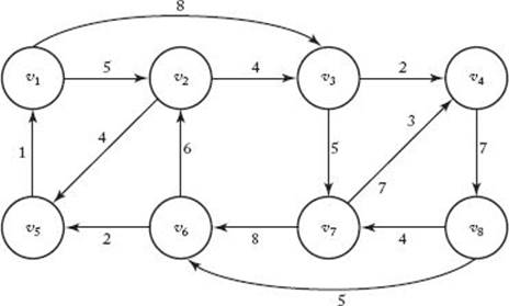
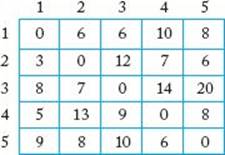
Recall that the goal in this problem is to find the shortest path in a directed graph that starts at a given vertex, visits each vertex in the graph exactly once, and ends up back at the starting vertex. Such a path is called an optimal tour. Because it does not matter where we start, the starting vertex can simply be the first vertex. Figure 6.4 shows the adjacency matrix representation of a graph containing five vertices, in which there is an edge from every vertex to every other vertex, and an optimal tour for that graph.
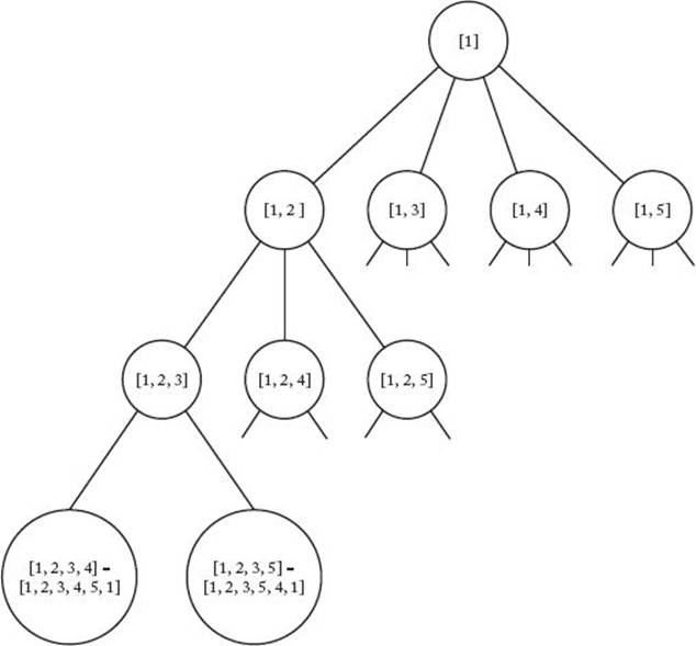
An obvious state space tree for this problem is one in which each vertex other than the starting one is tried as the first vertex (after the starting one) at level 1, each vertex other than the starting one and the one chosen at level 1 is tried as the second vertex at level 2, and so on. A portion of this state space tree, in which there are five vertices and in which there is an edge from every vertex to every other vertex, is shown in Figure 6.5. In what follows, the term “node” means a node in the state space tree, and the term “vertex” means a vertex in the graph. At each node in Figure 6.5, we have included the path chosen up to that node. For simplicity, we have denoted a vertex in the graph simply by its index. A node that is not a leaf represents all those tours that start with the path stored at that node. For example, the node containing [1, 2, 3] represents all those tours that start with the path [1, 2, 3]. That is, it represents the tours [1, 2, 3, 4, 5, 1] and [1, 2, 3, 5, 4, 1]. Each leaf represents a tour. We need to find a leaf that contains an optimal tour. We stop expanding the tree when there are four vertices in the path stored at a node because, at that time, the fifth one is uniquely determined. For example, the far-left leaf represents the tour [1, 2, 3, 4, 5, 1 ] because once we have specified the path [1, 2, 3, 4], the next vertex must be the fifth one.
Figure 6.4 Adjacency matrix representation of a graph that has an edge from every vertex to every other vertex (left), and the nodes in the graph and the edges in an optimal tour (right).
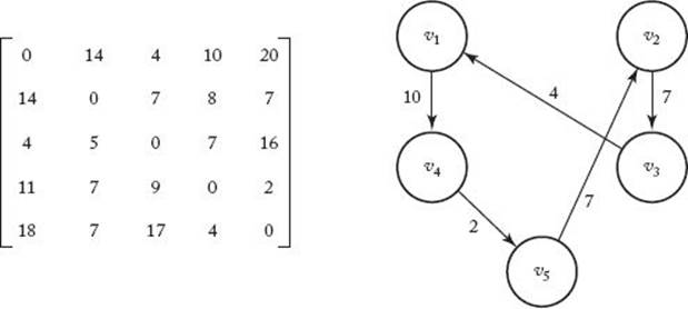
Figure 6.5 A state space tree for an instance of the Traveling Salesperson problem in which there are five vertices. The indices of the vertices in the partial tour are stored at each node.
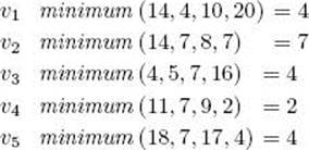
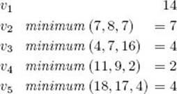
To use best-first search, we need to be able to determine a bound for each node. Because of the objective in the 0-1 Knapsack problem (to maximize profit while keeping the total weight from exceeding W), we computed an upper bound on the amount of profit that could be obtained by expanding beyond a given node, and we called a node promising only if its bound was greater than the current maximum profit. In this problem, we need to determine a lower bound on the length of any tour that can be obtained by expanding beyond a given node, and we call the node promising only if its bound is less than the current minimum tour length. We can obtain a bound as follows. In any tour, the length of the edge taken when leaving a vertex must be at least as great as the length of the shortest edge emanating from that vertex. Therefore, a lower bound on the cost (length of the edge taken) of leaving vertex v1 is given by the minimum of all the nonzero entries in row 1 of the adjacency matrix, a lower bound on the cost of leaving vertex v2 is given by the minimum of all the nonzero entries in row 2, and so on. The lower bounds on the costs of leaving the five vertices in the graph represented in Figure 6.4 are as follows:
Because a tour must leave every vertex exactly once, a lower bound on the length of a tour is the sum of these minimums. Therefore, a lower bound on the length of a tour is
![]()
This is not to say that there is a tour with this length. Rather, it says that there can be no tour with a shorter length.
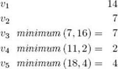
Suppose we have visited the node containing [1, 2] in Figure 6.5. In that case we have already committed to making v2 the second vertex on the tour, and the cost of getting to v2 is the weight on the edge from v1 to v2, which is 14. Any tour obtained by expanding beyond this node, therefore, has the following lower bounds on the costs of leaving the vertices:
To obtain the minimum for v2 we do not include the edge to v1, because v2 cannot return to v1. To obtain the minimums for the other vertices we do not include the edge to v2, because we have already been at v2. A lower bound on the length of any tour, obtained by expanding beyond the node containing [1, 2], is the sum of these minimums, which is
![]()
To further illustrate the technique for determining the bound, suppose we have visited the node containing [1, 2, 3] in Figure 6.5. We have committed to making v2 the second vertex and v3 the third vertex. Any tour obtained by expanding beyond this node has the following lower bounds on the costs of leaving the vertices:
To obtain the minimums for v4 and v5 we do not consider the edges to v2 and v3, because we have already been to these vertices. The lower bound on the length of any tour we could obtain by expanding beyond the node containing [1, 2, 3] is
![]()
In the same way, we can obtain a lower bound on the length of a tour that can be obtained by expanding beyond any node in the state space tree, and we use these lower bounds in our best-first search. The following example illustrates this technique. We will not actually do any calculations in the example. They would be done as just illustrated.
Example 6.3
Given the graph in Figure 6.4 and using the bounding considerations outlined previously, a best-first search with branch-and-bound pruning produces the tree in Figure 6.6. The bound is stored at a nonleaf, whereas the length of the tour is stored at a leaf. We show the steps that produced the tree. We initialize the value of the best solution to ∞ (infinity) because there is no candidate solution at the root. (Candidate solutions exist only at leaves in the state space tree.) We do not compute bounds for leaves in the state space tree because the algorithm is written so as not to expand beyond leaves. When referring to a node, we refer to the partial tour stored at the node. This is different from the way we referred to a node when illustrating the 0-1 Knapsack problem.
The steps are as follows:
1. Visit node containing [1] (the root).
(a) Compute bound to be 21.
(b) Set minlength to ∞.
{This is a lower bound on the}
{length of a tour.}
2. Visit node containing [1, 2].
(a) Compute bound to be 31.
3. Visit node containing [1, 3].
(a) Compute bound to be 22.
4. Visit node containing [1, 4].
(a) Compute bound to be 30.
5. Visit node containing [1, 5].
(a) Compute bound to be 42.
6. Determine promising, unexpanded node with the smallest bound.
(a) That node is the node containing [1, 3]. We visit its children next.
7. Visit node containing [1, 3, 2].
(a) Compute bound to be 22.
Figure 6.6 The pruned state space tree produced using best-first search with branch-and-bound pruning in Example 6.3. At each node that is not a leaf in the state space tree, the partial tour is at the top and the bound on the length of any tour that could be obtained by expanding beyond the node is at the bottom. At each leaf in the state space tree, the tour is at the top and its length is at the bottom. The node shaded in color is the one at which an optimal tour is found.
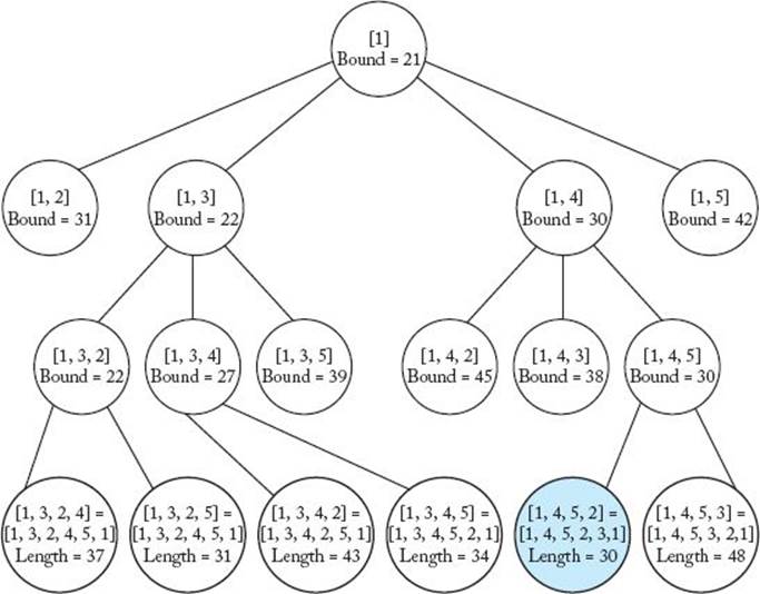
8. Visit node containing [1, 3, 4].
(a) Compute bound to be 27.
9. Visit node containing [1, 3, 5].
(a) Compute bound to be 39.
10. Determine promising, unexpanded node with the smallest bound.
(a) That node is the node containing [1, 3, 2]. We visit its children next.
11. Visit node containing [1,3,2,4].
(a) Because this node is a leaf, compute tour length to be 37.
(b) Because its length 37 is less than ∞, the value of minlength, set minlength to 37.
(c) The nodes containing [1, 5] and [1, 3, 5] become nonpromising because their bounds 42 and 39 are greater than or equal to 37, the new value of minlength.
12. Visit node containing [1, 3, 2, 5].
(a) Because this node is a leaf, compute tour length to be 31.
(b) Because its length 31 is less than 37, the value of minlength, set minlength to 31.
(c) The node containing [1, 2] becomes nonpromising because its bound 31 is greater than or equal to 31, the new value of minlength.
13. Determine promising, unexpanded node with the smallest bound.
(a) That node is the node containing [1, 3, 4]. We visit its children next.
14. Visit node containing [1, 3, 4, 2].
(a) Because this node is a leaf, compute tour length to be 43.
15. Visit node containing [1, 3, 4, 5].
(a) Because this node is a leaf, compute tour length to be 34.
16. Determine promising, unexpanded node with the smallest bound.
(a) The only promising, unexpanded node is the node containing [1, 4]. We visit its children next.
17. Visit node containing [1, 4, 2].
(a) Compute bound to be 45.
(b) Determine that the node is nonpromising because its bound 45 is greater than or equal to 31, the value of minlength.
18. Visit node containing [1, 4, 3].
(a) Compute bound to be 38.
(b) Determine that the node is nonpromising because its bound 38 is greater than or equal to 31, the value of minlength.
19. Visit node containing [1, 4, 5].
(a) Compute bound to be 30.
20. Determine promising, unexpanded node with the smallest bound.
(a) The only promising, unexpanded node is the node containing [1, 4, 5]. We visit its children next.
21. Visit node containing [1, 4, 5, 2].
(a) Because this node is a leaf, compute tour length to be 30.
(b) Because its length 30 is less than 31, the value of minlength, set minlength to 30.
22. Visit node containing [1, 4, 5, 3].
(a) Because this node is a leaf, compute tour length to be 48.
23. Determine promising, unexpanded node with the smallest bound.
(a) There are no more promising, unexpanded nodes. We are done.
We have determined that the node containing [1, 4, 5, 2], which represents the tour [1,4, 5, 2, 3, 1], contains an optimal tour, and that the length of an optimal tour is 30.
There are 17 nodes in the tree in Figure 6.6, whereas the number of nodes in the entire state space tree is 1 + 4 + 4 × 3 + 4 × 3 × 2 = 41.
We will use the following data type in the algorithm that implements the strategy used in the previous example:
The field path contains the partial tour stored at the node. For example, in Figure 6.6 the value of path for the far left child of the root is [1, 2]. The algorithm follows.
![]() Algorithm 6.3
Algorithm 6.3
The Best-First Search with Branch-and-Bound Pruning Algorithm for the Traveling Salesperson problem
Problem: Determine an optimal tour in a weighted, directed graph. The weights are nonnegative numbers.
Inputs: a weighted, directed graph, and n, the number of vertices in the graph. The graph is represented by a two-dimensional array W , which has both its rows and columns indexed from 1 to n, where W [i] [j] is the weight on the edge from the ith vertex to the jth vertex.
Outputs: variable minlength, whose value is the length of an optimal tour, and variable opttour, whose value is an optimal tour.
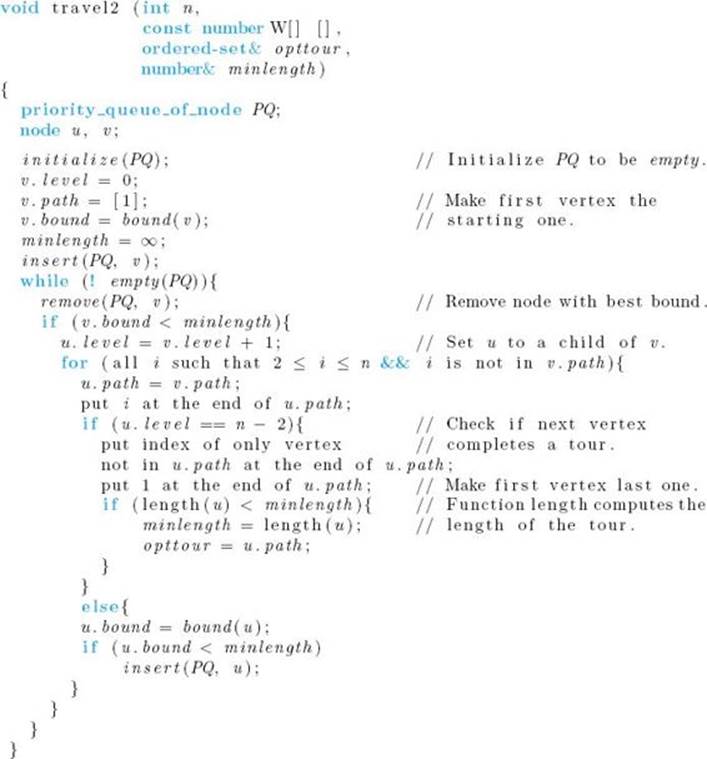
You are asked to write functions length and bound in the exercises. Function length returns the length of the tour u.path, and function bound returns the bound for a node using the considerations discussed.
A problem does not necessarily have a unique bounding function. In the Traveling Salesperson problem, for example, we could observe that every vertex must be visited exactly once, and then use the minimums of the values in the columns in the adjacency matrix instead of the minimums of the values in the rows. Alternatively, we could take advantage of both the rows and the columns by noting that every vertex must be entered and exited exactly once. For a given edge, we could associate half of its weight with the vertex it leaves and the other half with the vertex it enters. The cost of visiting a vertex is then the sum of the weights associated with entering and exiting it. For example, suppose we are determining the initial bound on the length of a tour. The minimum cost of entering v2 is obtained by taking 1/2 of the minimum of the values in the second column. The minimum cost of exiting v2 is obtained by taking 1/2 of the minimum of the values in the second row. The minimum cost of visiting v2 is then given by
![]()
Using this bounding function, a branch-and-bound algorithm checks only 15 vertices in the instance in Example 6.3.
When two or more bounding functions are available, one bounding function may produce a better bound at one node whereas another produces a better bound at another node. Indeed, as you are asked to verify in the exercises, this is the case for our bounding functions for the Traveling Sales-person problem. When this is the case, the algorithm can compute bounds using all available bounding functions, and then use the best bound. However, as discussed in Chapter 5, our goal is not to visit as few nodes as possible, but rather to maximize the overall efficiency of the algorithm. The extra computations done when using more than one bounding function may not be offset by the savings realized by visiting fewer nodes.
Recall that a branch-and-bound algorithm might solve one large instance efficiently but check an exponential (or worse) number of nodes for another large instance. Returning to Nancy’s dilemma, what is she to do if even the branch-and-bound algorithm cannot solve her 40-city instance efficiently? Another approach to handling problems such as the Traveling Salesperson problem is to develop approximation algorithms. Approximation algorithms are not guaranteed to yield optimal solutions, but rather yield solutions that are reasonably close to optimal. They are discussed in Section 9.5. In that section we return to the Traveling Salesperson problem.
![]() 6.3 Abductive Inference (Diagnosis)
6.3 Abductive Inference (Diagnosis)
This section requires knowledge of discrete probability theory and Bayes’ theorem.
An important problem in artificial intelligence and expert systems is determining the most probable explanation for some findings. For example, in medicine we want to determine the most probable set of diseases, given a set of symptoms. In the case of an electronic circuit, we want to find the most probable explanation for a failure at some point in the circuit. Another example is the determination of the most probable causes for the failure of an automobile to function properly. This process of determining the most probable explanation for a set of findings is called abductive inference.
For the sake of focus, we use medical terminology. Assume that there are n diseases, d1, d2, … , dn, each of which may be present in a patient. We know that the patient has a certain set of symptoms S. Our goal is to find the set of diseases that are most probably present. Technically, there could be two or more sets that are probably present. However, we often discuss the problem as if a unique set is most probably present.
The Bayesian network has become a standard for representing probabilistic relationships such as those between diseases and symptoms. It is beyond our scope to discuss belief networks here. They are discussed in detail in Neapolitan (1990, 2003) and Pearl (1988). For many Bayesian network applications, there exist efficient algorithms for determining the prior probability (before any symptoms are discovered) that a particular set of diseases contains the only diseases present in the patient. These algorithms are also discussed in Neapolitan (1990, 2003) and Pearl (1988). Here we will simply assume that the results of the algorithms are available to us. For example, these algorithms can determine the prior probability that d1, d3, and d6 are the only diseases present in the patient. We will denote this probability by
![]()
where
![]()
These algorithms can also determine the probability that d1, d3, and d6 are the only diseases present, conditional on the information that the symptoms in S are present. We will denote this conditional probability by
![]()
Given that we can compute these probabilities (using the algorithms mentioned previously), we can solve the problem of determining the most probable set of diseases (conditional on the information that some symptoms are present) using a state space tree like the one in the 0-1 Knapsack problem. We go to the left of the root to include d1, and we go to the right to exclude it. Similarly, we go to the left of a node at level 1 to include d2, and we go to the right to exclude it, and so on. Each leaf in the state space tree represents a possible solution (that is, the set of diseases that have been included up to that leaf). To solve the problem, we compute the conditional probability of the set of diseases at each leaf, and determine which one has the largest conditional probability.
To prune using best-first search, we need to find a bounding function. The following theorem accomplishes this for a large class of instances.
![]() Theorem 6.1
Theorem 6.1
If D and D’ are two sets of diseases such that
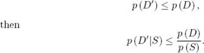
Proof: According to Bayes’ theorem,
The first inequality is by the assumption in this theorem, and the second follows from the fact that any probability is less than or equal to 1. This proves the theorem.
For a given node, let D be the set of diseases that have been included up to that node, and for some descendant of that node, let D’ be the set of diseases that have been included up to that descendant. Then D ⊆ D’. Often it is reasonable to assume that
![]()
The reason is that usually it is at least as probable that a patient has a set of diseases as it is that the patient has that set plus even more diseases. (Recall that these are prior probabilities before any symptoms are observed.) If we make this assumption, by Theorem 6.1,
Therefore, p (D) /p (S) is an upper bound on the conditional probability of the set of diseases in any descendant of the node. The following example illustrates how this bound is used to prune branches.
Example 6.4
Suppose there are four possible diseases d1, d2, d3, and d4 and a set of symptoms S. The input to this example would also include a Bayesian network containing the probabilistic relationships among the diseases and the symptoms. The probabilities used in this example would be computed from this Bayesian network using the methods discussed earlier. These probabilities are not computed elsewhere in this text. We assign arbitrary probabilities to illustrate the best-first search algorithm. When using the results from one algorithm (in this case, the one for doing inference in a belief network) in another algorithm (in this case, the best-first search algorithm), it is important to recognize where the first algorithm supplies results that can simply be assumed in the second algorithm.
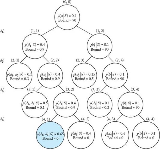
Figure 6.7 is the pruned state space tree produced by a best-first search. Probabilities have been given arbitrary values in the tree. The conditional probability is at the top and the bound is at the bottom in each node. The node shaded in color is the one at which the best solution is found. As was done in Section 6.1, nodes are labeled according to their depth and position from the left in the tree. The steps that produce the tree follow. The variable best is the current best solution, whereas p (best | S) is its conditional probability. Our goal is to determine a value of best that maximizes this conditional probability. It is also assumed arbitrarily that
Figure 6.7 The pruned state space tree produced using best-first search with branch-and-bound pruning in Example 6.4. At each node, the conditional probability of the diseases included up to that node is at the top, and the bound on the conditional probability that could be obtained by expanding beyond the node is at the bottom. The node shaded in color is the one at which an optimal set is found.
![]()
1. Visit node (0, 0) (the root).
(a) Compute its conditional probability. {∅ is the empty set. This means that no diseases are present.}

(b) Set
![]()
(c) Compute its prior probability and bound.
2. Visit node (1, 1).
(a) Compute its conditional probability.
![]()
(b) Because 0.4 > p (best|S), set
![]()
(c) Compute its prior probability and bound.
3. Visit node (1, 2).
(a) Its conditional probability is simply that of its parent—namely, 0.1.
(b) Its prior probability and bound are simply those of its parent— namely, 0.9 and 90.
4. Determine promising, unexpanded node with the largest bound.
(a) That node is node (1, 2). We visit its children next.
5. Visit node (2, 3).
(a) Compute its conditional probability.
![]()
(b) Compute its prior probability and bound.
6. Visit node (2, 4).
(a) Its conditional probability is simply that of its parent—namely, 0.1.
(b) Its prior probability and bound are simply those of its parent— namely, .9 and 90.
7. Determine promising, unexpanded node with the largest bound.
(a) That node is node (2, 4). We visit its children next.
8. Visit node (3, 3).
(a) Compute its conditional probability.
![]()
(b) Compute its conditional probability and bound.
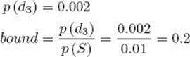
(c) Determine that it is nonpromising because its bound .2 is less than or equal to .4, the value of p (best|S).
9. Visit node (3, 4).
(a) Its conditional probability is simply that of its parent—namely, 0.1.
(b) Its prior probability and bound are simply those of its parent– namely, 0.9 and 90.
10. Determine promising, unexpanded node with the largest bound.
(a) That node is node (3, 4). We visit its children next.
11. Visit node (4, 3).
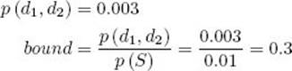
(a) Compute its conditional probability.
![]()
(b) Because 0.6 > p (best|S), set
![]()
(c) Set its bound to 0 because it is a leaf in the state space tree.
(d) At this point, the node (2, 3) becomes nonpromising because its bound 0.5 is less than or equal to 0.6, the new value of p (best|S).
12. Visit node (4, 4).
(a) Its conditional probability is simply that of its parent—namely, 0.1.
(b) Set its bound to 0 because it is a leaf in the state space tree.
13. Determine promising, unexpanded node with the largest bound.
(a) That node is node (1, 1). We visit its children next.
14. Visit node (2, 1).
(a) Compute its conditional probability.
![]()
(b) Compute its prior probability and bound.
(c) Determine that it is nonpromising because its bound 0.3 is less than or equal to 0.6, the value of p (best|S).
15. Visit node (2, 2).
(a) Its conditional probability is simply that its parent–namely, 0.4.
(b) Its prior probability and bound are simply those of its parent–namely, 0.009 and 0.9.
16. Determine promising, unexpanded node with the greatest bound.
(a) The only promising, unexpanded node is node (2, 2). We visit its children next.
17. Visit node (3, 1).
(a) Compute its conditional probability.
![]()
(b) Compute its prior probability and bound.
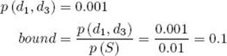
(c) Determine that it is nonpromising because its bound 0.1 is less than or equal to 0.6, the value of p (best|S).
18. Visit node (3, 2).
(a) Its conditional probability is simply that of its parent—namely, 0.4.
(b) Its prior probability and found are simply those of its parent— namely, 0.009 and 0.9.
19. Determine promising, unexpanded node with the largest bound.
(a) The only promising, unexpanded node is node (3, 2). We visit its children next.
20. Visit node (4, 1).
(a) Compute its conditional probability.
![]()
(b) Because 0.65 > p (best|S), set
![]()
(c) Set its bound to 0 because it is a leaf in the state space tree.
21. Visit node (4, 2).
(a) Its conditional probability is simply that of its parent—namely, 0.4.
(b) Set its bound to 0 because it is a leaf in the state space tree.
22. Determine promising, unexpanded node with the largest bound.
(a) There are no more promising, unexpanded nodes. We are done.
We have determined that the most probable set of diseases is {d1, d4} and that p (d1, d4|S) = 0.65.
A reasonable strategy in this problem would be to initially sort the diseases in nonincreasing order according to their conditional probabilities. There is no guarantee, however, that this strategy will minimize the search time. We have not done this in Example 6.4, and 15 nodes were checked. In the exercises, you establish that if the diseases were sorted, 23 nodes would be checked.
Next we present the algorithm. It uses the following declaration:
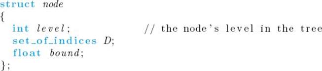
The field D contains the indices of the diseases included up to the node. One of the inputs to this algorithm is a Bayesian network BN. As mentioned previously, a Bayesian network represents the probabilistic relationships among diseases and symptoms. The algorithms referenced at the beginning of this section can compute the necessary probabilities from such a network.
The following algorithm was developed by Cooper (1984):
![]() Algorithm 6.4
Algorithm 6.4
Cooper’s Best-First Search with Branch-and-Bound Pruning Algorithm for Abductive Inference
Problem: Determine a most probable set of diseases (explanation) given a set of symptoms. It is assumed that if a set of diseases D is a subset of a set of diseases D’, then p (D’) ≤ p (D).
Inputs: positive integer n, a Bayesian network BN representing the probabilistic relationships among n diseases and their symptoms, and a set of symptoms S.
Outputs: a set best containing the indices of the diseases in a most probable set (conditional on S), and a variable pbest that is the probability of best given S.
The notation p (D) stands for the prior probability of D, p (S) stands for the prior probability of S, and p (D|S) stands for the conditional probability of D given S. These values would be computed from the Bayesian network BN using the algorithms referenced at the beginning of this section.
We have written the algorithm strictly according to our guidelines for writing best-first search algorithms. An improvement is possible. There is no need to call function bound for the right child of a node. The reason is that the right child contains the same set of diseases as the node itself, which means that its bound is the same. Therefore, the right child is pruned only if, at the left child, we change pbest to a value greater than or equal to this bound. We can modify our algorithm to prune the right child when this happens and to expand to the right child when it does not happen.
Like the other problems described in this chapter, the problem of Abductive Inference is in the class of problems discussed in Chapter 9.
If there is more than one solution, the preceding algorithm only produces one of them. It is straightforward to modify the algorithm to produce all the best solutions. It is also possible to modify it to produce the m most probable explanations, where m is any positive integer. This modification is discussed in Neapolitan (1990). Furthermore, Neapolitan (1990) analyzes the algorithm in detail.
EXERCISES
Section 6.1
1. Use Algorithm 6.1 (The Breadth-First Search with Branch-and-Bound Pruning algorithm for the 0-1 Knapsack problem) to maximize the profit for the following problem instance. Show the actions step by step.
2. Implement Algorithm 6.1 on your system and run it on the problem instance of Exercise 1.
3. Modify Algorithm 6.1 to produce an optimal set of items. Compare the performance of your algorithm with that of Algorithm 6.1.
4. Use Algorithm 6.2 (The Best-First Search with Branch-and-Bound Pruning algorithm for the 0-1 Knapsack problem) to maximize the profit for the problem instance of Exercise 1. Show the actions step by step.
5. Implement Algorithm 6.2 on your system and run it on the problem instance of Exercise 1.
6. Compare the performance of Algorithm 6.1 with that of Algorithm 6.2 for large instances of the problem.
Section 6.2
7. Use Algorithm 6.3 (The Best-First Search with Branch-and-Bound Pruning Algorithm for the Traveling Salesperson problem) to find an optimal tour and the length of the optimal tour for the graph below.
Show the actions step by step.
8. Use Algorithm 6.3 to find an optimal tour for the graph whose adjacency matrix is given by the following array. Show your actions step by step.
9. Write functions length and bound used in Algorithm 6.3.
10. Consider the Traveling Salesperson problem.
(a) Write the brute-force algorithm for this problem that considers all possible tours.
(b) Implement the algorithm and use it to solve instances of size 6, 7, 8, 9, 10, 15, and 20.
(c) Compare the performance of this algorithm to that of Algorithm 6.3 using the instances developed in (b).
11. Implement Algorithm 6.3 on your system, and run it on the problem instance of Exercise 7. Use different bounding functions and study the results.
12. Compare the performance of your dynamic programming algorithm (see Section 3.6, Exercise 27) for the Traveling Salesperson problem with that of Algorithm 6.3 using large instances of the problem.
Section 6.3
13. Revise Algorithm 6.4 (Cooper’s Best-First Search with Branch-and-Bound Pruning algorithm for Abductive Inference) to produce the m most probable explanations, where m is any positive integer.
14. Show that if the diseases in Example 6.4 were sorted in nonincreasing order according to their conditional probabilities, the number of nodes checked would be 23 instead of 15. Assume that p(d4) = 0.008 and p (d4, d1) = 0.007.
15. A set of explanations satisfies a comfort measure p if the sum of the probabilities of the explanations is greater than or equal to p. Revise Algorithm 6.4 to produce a set of explanations that satisfies p, where 0 ≤ p ≤ 1. Do this with as few explanations as possible.
16. Implement Algorithm 6.4 on your system. The user should be able to enter an integer m, as described in Exercise 11, or a comfort measure p, as described in Exercise 13.
Additional Exercises
17. Can the branch-and-bound design strategy be used to solve the problem discussed in Exercise 34 in Chapter 3? Justify your answer.
18. Write a branch-and-bound algorithm for the problem of scheduling with deadlines discussed in Section 4.3.2.
19. Can the branch-and-bound design strategy be used to solve the problem discussed in Exercise 26 in Chapter 4? Justify your answer.
20. Can the branch-and-bound design strategy be used to solve the Chained Matrix Multiplication problem discussed in Section 3.4? Justify your answer.
21. List three more applications of the branch-and-bound design strategy.
All materials on the site are licensed Creative Commons Attribution-Sharealike 3.0 Unported CC BY-SA 3.0 & GNU Free Documentation License (GFDL)
If you are the copyright holder of any material contained on our site and intend to remove it, please contact our site administrator for approval.
© 2016-2026 All site design rights belong to S.Y.A.