Algorithms (2014)
Three. Searching
3.2 Binary Search Trees
IN THIS SECTION, we will examine a symbol-table implementation that combines the flexibility of insertion in a linked list with the efficiency of search in an ordered array. Specifically, using two links per node (instead of the one link per node found in linked lists) leads to an efficient symbol-table implementation based on the binary search tree data structure, which qualifies as one of the most fundamental algorithms in computer science.
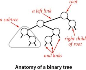
To begin, we define basic terminology. We are working with data structures made up of nodes that contain links that are either null or references to other nodes. In a binary tree, we have the restriction that every node is pointed to by just one other node, which is called its parent (except for one node, the root, which has no nodes pointing to it), and that each node has exactly two links, which are called its left and right links, that point to nodes called its left child and right child, respectively. Although links point to nodes, we can view each link as pointing to a binary tree, the tree whose root is the referenced node. Thus, we can define a binary tree as either a null link or a node with a left link and a right link, each references to (disjoint) subtrees that are themselves binary trees. In a binary search tree, each node also has a key and a value, with an ordering restriction to support efficient search.
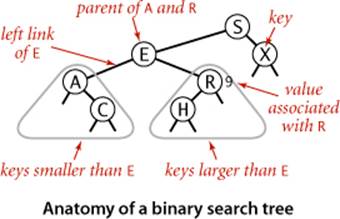
Definition. A binary search tree (BST) is a binary tree where each node has a Comparable key (and an associated value) and satisfies the restriction that the key in any node is larger than the keys in all nodes in that node’s left subtree and smaller than the keys in all nodes in that node’s right subtree.
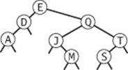
We draw BSTs with keys in the nodes and use terminology such as “A is the left child of E” that associates nodes with keys. Lines connecting the nodes represent links, and we give the value associated with a key in black, beside the nodes (suppressing the value as dictated by context). Each node’s links connect it to nodes below it on the page, except for null links, which are short segments at the bottom. As usual, our examples use the single-letter keys that are generated by our indexing test client.
Basic implementation
ALGORITHM 3.3 defines the BST data structure that we use throughout this section to implement the ordered symbol-table API. We begin by considering this classic data structure definition and the characteristic associated implementations of the get() (search) and put() (insert) methods.
Representation
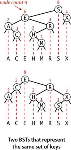
We define a private nested class to define nodes in BSTs, just as we did for linked lists. Each node contains a key, a value, a left link, a right link, and a node count (when relevant, we include node counts in red above the node in our drawings). The left link points to a BST for items with smaller keys, and the right link points to a BST for items with larger keys. The instance variable N gives the node count in the subtree rooted at the node. This field facilitates the implementation of various ordered symbol-table operations, as you will see. The private size() method inALGORITHM 3.3 is implemented to assign the value 0 to null links, so that we can maintain this field by making sure that the invariant
size(x) = size(x.left) + size(x.right) + 1
holds for every node x in the tree.
A BST represents a set of keys (and associated values), and there are many different BSTs that represent the same set. If we project the keys in a BST such that all keys in each node’s left subtree appear to the left of the key in the node and all keys in each node’s right subtree appear to the right of the key in the node, then we always get the keys in sorted order. We take advantage of the flexibility inherent in having many BSTs represent this sorted order to develop efficient algorithms for building and using BSTs.
Search
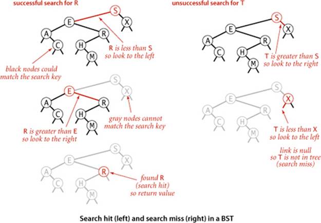
As usual, when we search for a key in a symbol table, we have one of two possible outcomes. If a node containing the key is in the table, we have a search hit, so we return the associated value. Otherwise, we have a search miss (and return null). A recursive algorithm to search for a key in a BST follows immediately from the recursive structure: if the tree is empty, we have a search miss; if the search key is equal to the key at the root, we have a search hit. Otherwise, we search (recursively) in the appropriate subtree, moving left if the search key is smaller, right if it is larger. The recursive get() method on page 399 implements this algorithm directly. It takes a node (root of a subtree) as first argument and a key as second argument, starting with the root of the tree and the search key. The code maintains the invariant that no parts of the tree other than the subtree rooted at the current node can have a node whose key is equal to the search key. Just as the size of the interval in binary search shrinks by about half on each iteration, the size of the subtree rooted at the current node when searching in a BST shrinks when we go down the tree (by about half, ideally, but at least by one). The procedure stops either when a node containing the search key is found (search hit) or when the current subtree becomes empty (search miss). Starting at the top, the search procedure at each node involves a recursive invocation for one of that node’s children, so the search defines a path through the tree. For a search hit, the path terminates at the node containing the key. For a search miss, the path terminates at a null link.
Algorithm 3.3 Binary search tree symbol table
public class BST<Key extends Comparable<Key>, Value>
{
private Node root; // root of BST
private class Node
{
private Key key; // key
private Value val; // associated value
private Node left, right; // links to subtrees
private int N; // # nodes in subtree rooted here
public Node(Key key, Value val, int N)
{ this.key = key; this.val = val; this.N = N; }
}
public int size()
{ return size(root); }
private int size(Node x)
{
if (x == null) return 0;
else return x.N;
}
public Value get(Key key)
// See page 399.
public void put(Key key, Value val)
// See page 399.
// See page 407 for min(), max(), floor(), and ceiling().
// See page 409 for select() and rank().
// See page 411 for delete(), deleteMin(), and deleteMax().
// See page 413 for keys().
}
This implementation of the ordered symbol-table API uses a binary search tree built from Node objects that each contain a key, associated value, two links, and a node count N. Each Node is the root of a subtree containing N nodes, with its left link pointing to a Node that is the root of a subtree with smaller keys and its right link pointing to a Node that is the root of a subtree with larger keys. The instance variable root points to the Node at the root of the BST (which has all the keys and associated values in the symbol table). Implementations of other methods appear throughout this section.
Algorithm 3.3 Search and insert for BSTs
public Value get(Key key)
{ return get(root, key); }
private Value get(Node x, Key key)
{ // Return value associated with key in the subtree rooted at x;
// return null if key not present in subtree rooted at x.
if (x == null) return null;
int cmp = key.compareTo(x.key);
if (cmp < 0) return get(x.left, key);
else if (cmp > 0) return get(x.right, key);
else return x.val;
}
public void put(Key key, Value val)
{ // Search for key. Update value if found; grow table if new.
root = put(root, key, val);
}
private Node put(Node x, Key key, Value val)
{
// Change key's value to val if key in subtree rooted at x.
// Otherwise, add new node to subtree associating key with val.
if (x == null) return new Node(key, val, 1);
int cmp = key.compareTo(x.key);
if (cmp < 0) x.left = put(x.left, key, val);
else if (cmp > 0) x.right = put(x.right, key, val);
else x.val = val;
x.N = size(x.left) + size(x.right) + 1;
return x;
}
These implementations of get() and put() for the symbol-table API are characteristic recursive BST methods that also serve as models for several other implementations that we consider later in the chapter. Each method can be understood as both working code and a proof by induction of the inductive hypothesis in the opening comment.
Insert
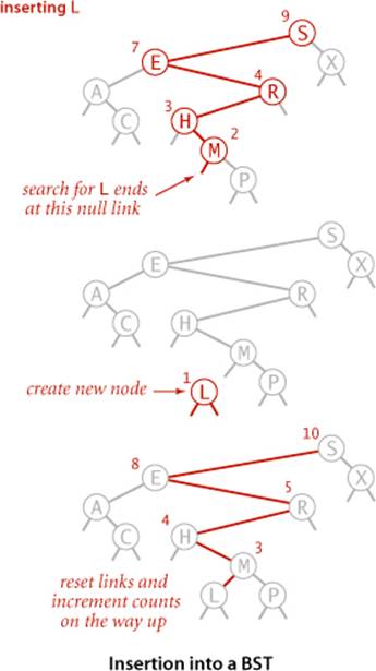
The search code in ALGORITHM 3.3 is almost as simple as binary search; that simplicity is an essential feature of BSTs. A more important essential feature of BSTs is that insert is not much more difficult to implement than search. Indeed, a search for a key not in the tree ends at a null link, and all that we need to do is replace that link with a new node containing the key (see the diagram on the next page). The recursive put() method in ALGORITHM 3.3 accomplishes this task using logic similar to that we used for the recursive search: if the tree is empty, we return a new node containing the key and value; if the search key is less than the key at the root, we set the left link to the result of inserting the key into the left subtree; otherwise, we set the right link to the result of inserting the key into the right subtree.
Recursion
It is worthwhile to take the time to understand the dynamics of these recursive implementations. You can think of the code before the recursive calls as happening on the way down the tree: it compares the given key against the key at each node and moves right or left accordingly. Then, think of the code after the recursive calls as happening on the way up the tree. For get() this amounts to a series of return statements, but for put(), it corresponds to resetting the link of each parent to its child on the search path and to incrementing the counts on the way up the path. In simple BSTs, the only new link is the one at the bottom, but resetting the links higher up on the path is as easy as the test to avoid setting them. Also, we just need to increment the node count on each node on the path, but we use more general code that sets each to one plus the sum of the counts in its subtrees. Later in this section and in the next section, we shall study more advanced algorithms that are naturally expressed with this same recursive scheme but that can change more links on the search paths and need the more general node-count-update code. Elementary BSTs are often implemented with nonrecursive code (see EXERCISE 3.2.13)—we use recursion in our implementations both to make it easy for you to convince yourself that the code is operating as described and to prepare the groundwork for more sophisticated algorithms.
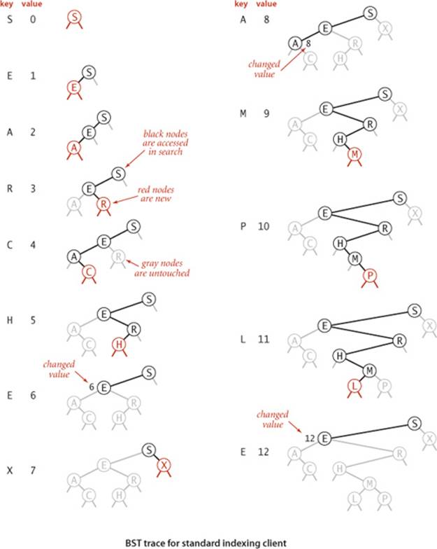
A CAREFUL STUDY of the trace for our standard indexing client that is shown on the next page will give you a feeling for the way in which binary search trees grow. New nodes are attached to null links at the bottom of the tree; the tree structure is not otherwise changed. For example, the root has the first key inserted, one of the children of the root has the second key inserted, and so forth. Because each node has two links, the tree tends to grow out, rather than just down. Moreover, only the keys on the path from the root to the sought or inserted key are examined, so the number of keys examined becomes a smaller and smaller fraction of the number of keys in the tree as the tree size increases.
Analysis
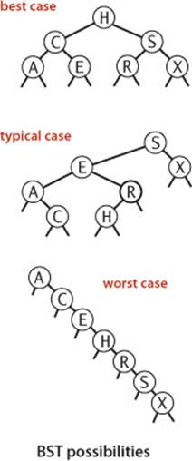
The running times of algorithms on binary search trees depend on the shapes of the trees, which, in turn, depend on the order in which keys are inserted. In the best case, a tree with N nodes could be perfectly balanced, with ~ lg N nodes between the root and each null link. In the worst case there could be N nodes on the search path. The balance in typical trees turns out to be much closer to the best case than the worst case.
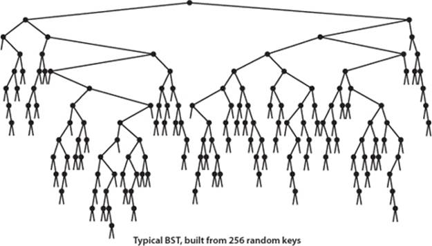
For many applications, the following simple model is reasonable: We assume that the keys are (uniformly) random, or, equivalently, that they are inserted in random order. Analysis of this model stems from the observation that BSTs are dual to quicksort. The node at the root of the tree corresponds to the first partitioning item in quicksort (no keys to the left are larger, and no keys to the right are smaller) and the subtrees are built recursively, corresponding to quicksort’s recursive subarray sorts. This observation leads us to the analysis of properties of the trees.
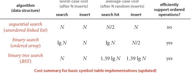
Proposition C. Search hits in a BST built from N random keys require ~ 2 ln N (about 1.39 lg N) compares, on the average.
Proof: The number of compares used for a search hit ending at a given node is 1 plus the depth. Adding the depths of all nodes, we get a quantity known as the internal path length of the tree. Thus, the desired quantity is 1 plus the average internal path length of the BST, which we can analyze with the same argument that we used for PROPOSITION K in SECTION 2.3: Let CN be the internal path length of a BST built from inserting N randomly ordered distinct keys, so that the average cost of a search hit is 1 +CN / N. We have C0 = C1 = 0 and for N > 1 we can write a recurrence relationship that directly mirrors the recursive BST structure:
CN = N − 1 + (C0 + CN−1) / N + (C1 + CN−2)/N + . . . (CN−1 + C0)/N
The N − 1 term takes into account that the root contributes 1 to the path length of each of the other N − 1 nodes in the tree; the rest of the expression accounts for the subtrees, which are equally likely to be any of the N sizes. After rearranging terms, this recurrence is nearly identical to the one that we solved in SECTION 2.3 for quicksort, and we can derive the approximation CN ~ 2N ln N.
Proposition D. Insertions and search misses in a BST built from N random keys require ~ 2 ln N (about 1.39 lg N) compares, on the average.
Proof: Insertions and search misses take one more compare, on the average, than search hits. This fact is not difficult to establish by induction (see EXERCISE 3.2.16).
PROPOSITION C says that we should expect the BST search cost for random keys to be about 39 percent higher than that for binary search. PROPOSITION D says that the extra cost is well worthwhile, because the cost of inserting a new key is also expected to be logarithmic—flexibility not available with binary search in an ordered array, where the number of array accesses required for an insertion is typically linear. As with quicksort, the standard deviation of the number of compares is known to be low, so that these formulas become increasingly accurate as N increases.
Experiments
How well does our random-key model match what is found in typical symbol-table clients? As usual, this question has to be studied carefully for particular practical applications, because of the large potential variation in performance. Fortunately, for many clients, the model is quite good for BSTs.
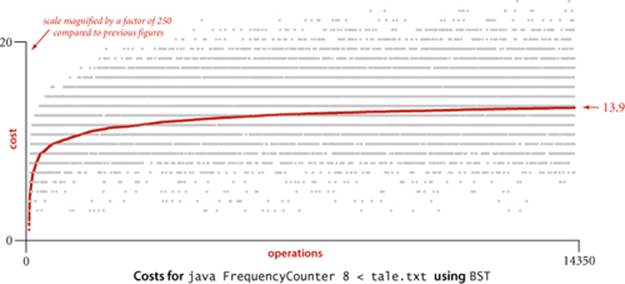
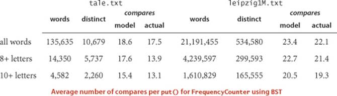
For our example study of the cost of the put() operations for FrequencyCounter for words of length 8 or more, we see a reduction in the average cost from 484 array accesses or compares per operation for BinarySearchST to 13 for BST, again providing a quick validation of the logarithmic performance predicted by the theoretical model. More extensive experiments for larger inputs are illustrated in the table on the next page. On the basis of PROPOSITIONS C and D, it is reasonable to predict that this number should be about twice the natural logarithm of the table size, because the preponderance of operations are searches in a nearly full table. This prediction has at least the following inherent inaccuracies:
• Many operations are for smaller tables.
• The keys are not random.
• The table size may be too small for the approximation 2 ln N to be accurate.
Nevertheless, as you can see in the table, this prediction is accurate for our FrequencyCounter test cases to within a few compares. Actually, most of the difference can be explained by refining the mathematics in the approximation (see EXERCISE 3.2.35).
Order-based methods and deletion
An important reason that BSTs are widely used is that they allow us to keep the keys in order. As such, they can serve as the basis for implementing the numerous methods in our ordered symbol-table API (see page 366) that allow clients to access key-value pairs not just by providing the key, but also by relative key order. Next, we consider implementations of the various methods in our ordered symbol-table API.
Minimum and maximum
If the left link of the root is null, the smallest key in a BST is the key at the root; if the left link is not null, the smallest key in the BST is the smallest key in the subtree rooted at the node referenced by the left link. This statement is both a description of the recursive min() method on page 407and an inductive proof that it finds the smallest key in the BST. The computation is equivalent to a simple iteration (move left until finding a null link), but we use recursion for consistency. We might have the recursive method return a Key instead of a Node, but we will later have a need to use this method to access the Node containing the minimum key. Finding the maximum key is similar, moving to the right instead of to the left.
Floor and ceiling
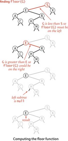
If a given key key is less than the key at the root of a BST, then the floor of key (the largest key in the BST less than or equal to key) must be in the left subtree. If key is greater than the key at the root, then the floor of key could be in the right subtree, but only if there is a key smaller than or equal to key in the right subtree; if not (or if key is equal to the key at the root), then the key at the root is the floor of key. Again, this description serves both as the basis for the recursive floor() method and for an inductive proof that it computes the desired result. Interchanging right and left (and lessand greater) gives ceiling().
Selection
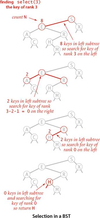
Selection in a BST works in a manner analogous to the partition-based method of selection in an array that we studied in SECTION 2.5. We maintain in BST nodes the variable N that counts the number of keys in the subtree rooted at that node precisely to support this operation. Suppose that we seek the key of rank k (the key such that precisely k other keys in the BST are smaller). If the number of keys t in the left subtree is larger than k, we look (recursively) for the key of rank k in the left subtree; if t is equal to k, we return the key at the root; and if t is smaller than k, we look (recursively) for the key of rank k − t − 1 in the right subtree. As usual, this description serves both as the basis for the recursive select() method on the facing page and for a proof by induction that it works as expected.
Algorithm 3.3 Min, max, floor, and ceiling in BSTs
public Key min()
{
return min(root).key;
}
private Node min(Node x)
{
if (x.left == null) return x;
return min(x.left);
}
public Key floor(Key key)
{
Node x = floor(root, key);
if (x == null) return null;
return x.key;
}
private Node floor(Node x, Key key)
{
if (x == null) return null;
int cmp = key.compareTo(x.key);
if (cmp == 0) return x;
if (cmp < 0) return floor(x.left, key);
Node t = floor(x.right, key);
if (t != null) return t;
else return x;
}
Each client method calls a corresponding private method that takes an additional link (to a Node) as argument and returns null or a Node containing the desired Key via the recursive procedure described in the text. The max() and ceiling() methods are the same as min() and floor() (respectively) with right and left (and < and >) interchanged.
Rank
The inverse method rank() that returns the rank of a given key is similar: if the given key is equal to the key at the root, we return the number of keys t in the left subtree; if the given key is less than the key at the root, we return the rank of the key in the left subtree (recursively computed); and if the given key is larger than the key at the root, we return t plus one (to count the key at the root) plus the rank of the key in the right subtree (recursively computed).
Delete the minimum/maximum
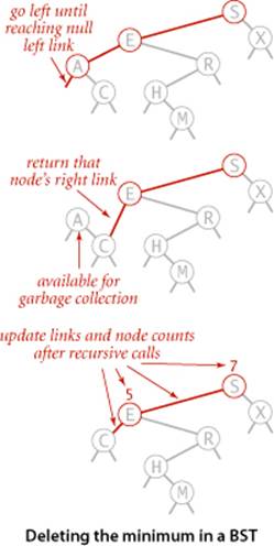
The most difficult BST operation to implement is the delete() method that removes a key-value pair from the symbol table. As a warmup, consider deleteMin() (remove the key-value pair with the smallest key). As with put() we write a recursive method that takes a link to a Node as argument and returns a link to a Node, so that we can reflect changes to the tree by assigning the result to the link used as argument. For deleteMin() we go left until finding a Node that has a null left link and then replace the link to that node by its right link (simply by returning the right link in the recursive method). The deleted node, with no link now pointing to it, is available for garbage collection. Our standard recursive setup accomplishes, after the deletion, the task of setting the appropriate link in the parent and updating the counts in all nodes in the path to the root. The symmetric method works for deleteMax().
Algorithm 3.3 Selection and rank in BSTs
public Key select(int k)
{
return select(root, k).key;
}
private Node select(Node x, int k)
{ // Return Node containing key of rank k.
if (x == null) return null;
int t = size(x.left);
if (t > k) return select(x.left, k);
else if (t < k) return select(x.right, k-t-1);
else return x;
}
public int rank(Key key)
{ return rank(key, root); }
private int rank(Key key, Node x)
{ // Return number of keys less than key in the subtree rooted at x.
if (x == null) return 0;
int cmp = key.compareTo(x.key);
if (cmp < 0) return rank(key, x.left);
else if (cmp > 0) return 1 + size(x.left) + rank(key, x.right);
else return size(x.left);
}
This code uses the same recursive scheme that we have been using throughout this chapter to implement the select() and rank() methods. It depends on using the private size() method given at the beginning of this section that returns the number of nodes in the subtree rooted at a node.
Delete
We can proceed in a similar manner to delete any node that has one child (or no children), but what can we do to delete a node that has two children? We are left with two links, but have a place in the parent node for only one of them. An answer to this dilemma, first proposed by T. Hibbard in 1962, is to delete a node x by replacing it with its successor. Because x has a right child, its successor is the node with the smallest key in its right subtree. The replacement preserves order in the tree because there are no keys between x.key and the successor’s key. We can accomplish the task of replacing x by its successor in four (!) easy steps:
• Save a link to the node to be deleted in t.
• Set x to point to its successor min(t.right).
• Set the right link of x (which is supposed to point to the BST containing all the keys larger than x.key) to deleteMin(t.right), the link to the BST containing all the keys that are larger than x.key after the deletion.
• Set the left link of x (which was null) to t.left (all the keys that are less than both the deleted key and its successor).
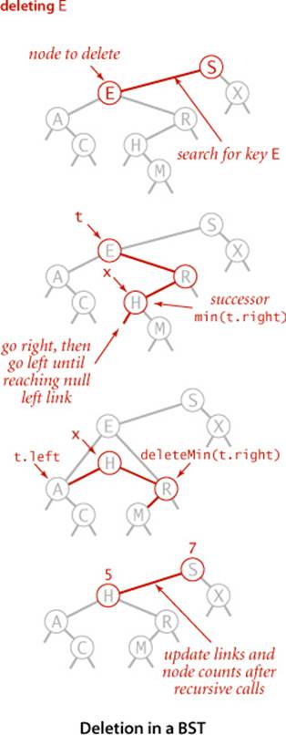
Our standard recursive setup accomplishes, after the recursive calls, the task of setting the appropriate link in the parent and decrementing the node counts in the nodes on the path to the root (again, we accomplish the task of updating the counts by setting the counts in each node on the search path to be one plus the sum of the counts in its children). While this method does the job, it has a flaw that might cause performance problems in some practical situations. The problem is that the choice of using the successor is arbitrary and not symmetric. Why not use the predecessor? In practice, it is worthwhile to choose at random between the predecessor and the successor. See EXERCISE 3.2.42 for details.
Algorithm 3.3 Deletion in BSTs
public void deleteMin()
{
root = deleteMin(root);
}
private Node deleteMin(Node x)
{
if (x.left == null) return x.right;
x.left = deleteMin(x.left);
x.N = size(x.left) + size(x.right) + 1;
return x;
}
public void delete(Key key)
{ root = delete(root, key); }
private Node delete(Node x, Key key)
{
if (x == null) return null;
int cmp = key.compareTo(x.key);
if (cmp < 0) x.left = delete(x.left, key);
else if (cmp > 0) x.right = delete(x.right, key);
else
{
if (x.right == null) return x.left;
if (x.left == null) return x.right;
Node t = x;
x = min(t.right); // See page 407.
x.right = deleteMin(t.right);
x.left = t.left;
}
x.N = size(x.left) + size(x.right) + 1;
return x;
}
These methods implement eager Hibbard deletion in BSTs, as described in the text on the facing page. The delete() code is compact, but tricky. Perhaps the best way to understand it is to read the description at left, try to write the code yourself on the basis of the description, then compare your code with this code. This method is typically effective, but performance in large-scale applications can become a bit problematic (see EXERCISE 3.2.42). The deleteMax() method is the same as deleteMin() with right and left interchanged.
Range queries
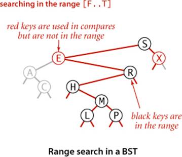
To implement the keys() method that returns the keys in a given range, we begin with a basic recursive BST traversal method, known as inorder traversal. To illustrate the method, we consider the task of printing all the keys in a BST in order. To do so, print all the keys in the left subtree (which are less than the key at the root by definition of BSTs), then print the key at the root, then print all the keys in the right subtree (which are greater than the key at the root by definition of BSTs), as in the code at left. As usual, the description serves as an argument by induction that this code prints the keys in order. To implement the two-argument keys() method that returns to a client all the keys in a specified range, we modify this code to add each key that is in the range to a Queue, and to skip the recursive calls for subtrees that cannot contain keys in the range. As withBinarySearchST, the fact that we gather the keys in a Queue is hidden from the client. The intention is that clients should process all the keys in the range of interest using Java’s foreach construct rather than needing to know what data structure we use to implement Iterable<Key>.
Printing the keys in a BST in order
private void print(Node x)
{
if (x == null) return;
print(x.left);
StdOut.println(x.key);
print(x.right);
}
Analysis
How efficient are the order-based operations in BSTs? To study this question, we consider the tree height (the maximum depth of any node in the tree). Given a tree, its height determines the worst-case cost of all BST operations (except for range search which incurs additional cost proportional to the number of keys returned).
Proposition E. In a BST, all operations take time proportional to the height of the tree, in the worst case.
Proof: All of these methods go down one or two paths in the tree. The length of any path is no more than the height, by definition.
We expect the tree height (the worst-case cost) to be higher than the average internal path length that we defined on page 403 (which averages in the short paths as well), but how much higher? This question may seem to you to be similar to the questions answered by PROPOSITION C andPROPOSITION D, but it is far more difficult to answer, certainly beyond the scope of this book. The average height of a BST built from random keys was shown to be logarithmic by J. Robson in 1979, and L. Devroye later showed that the value approaches 2.99 lg N for large N. Thus, if the insertions in our application are well-described by the random-key model, we are well on the way toward our goal of developing a symbol-table implementation that supports all of these operations in logarithmic time. We can expect that no path in a tree built from random keys is longer than 3 lg N, but what can we expect if the keys are not random? In the next section, you will see why this question is moot in practice because of balanced BSTs, which guarantee that the BST height will be logarithmic regardless of the order in which keys are inserted.
Algorithm 3.3 Range searching in BSTs
public Iterable<Key> keys()
{ return keys(min(), max()); }
public Iterable<Key> keys(Key lo, Key hi)
{
Queue<Key> queue = new Queue<Key>();
keys(root, queue, lo, hi);
return queue;
}
private void keys(Node x, Queue<Key> queue, Key lo, Key hi)
{
if (x == null) return;
int cmplo = lo.compareTo(x.key);
int cmphi = hi.compareTo(x.key);
if (cmplo < 0) keys(x.left, queue, lo, hi);
if (cmplo <= 0 && cmphi >= 0) queue.enqueue(x.key);
if (cmphi > 0) keys(x.right, queue, lo, hi);
}
To enqueue all the keys from the tree rooted at a given node that fall in a given range onto a queue, we (recursively) enqueue all the keys from the left subtree (if any of them could fall in the range), then enqueue the node at the root (if it falls in the range), then (recursively) enqueue all the keys from the right subtree (if any of them could fall in the range).
IN SUMMARY, BSTs are not difficult to implement and can provide fast search and insert for practical applications of all kinds if the key insertions are well-approximated by the random-key model. For our examples (and for many practical applications) BSTs make the difference between being able to accomplish the task at hand and not being able to do so. Moreover, many programmers choose BSTs for symbol-table implementations because they also support fast rank, select, delete, and range query operations. Still, as we have emphasized, the bad worst-case performance of BSTs may not be tolerable in some situations. Good performance of the basic BST implementation is dependent on the keys being sufficiently similar to random keys that the tree is not likely to contain many long paths. With quicksort, we were able to randomize; with a symbol-table API, we do not have that freedom, because the client controls the mix of operations. Indeed, the worst-case behavior is not unlikely in practice—it arises when a client inserts keys in order or in reverse order, a sequence of operations that some client certainly might attempt in the absence of any explicit warnings to avoid doing so. This possibility is a primary reason to seek better algorithms and data structures, which we consider next.
Q&A
Q. I’ve seen BSTs before, but not using recursion. What are the tradeoffs?
A. Generally, recursive implementations are a bit easier to verify for correctness; nonrecursive implementations are a bit more efficient. See EXERCISE 3.2.13 for an implementation of get(), the one case where you might notice the improved efficiency. If trees are unbalanced, the depth of the function-call stack could be a problem in a recursive implementation. Our primary reason for using recursion is to ease the transition to the balanced BST implementations of the next section, which definitely are easier to implement and debug with recursion.
Q. Maintaining the node count field in Node seems to require a lot of code. Is it really necessary? Why not maintain a single instance variable containing the number of nodes in the tree to implement the size() client method?
A. The rank() and select() methods need to have the size of the subtree rooted at each node. If you are not using these ordered operations, you can streamline the code by eliminating this field (see EXERCISE 3.2.12). Keeping the node count correct for all nodes is admittedly error-prone, but also a good check for debugging. You might also use a recursive method to implement size() for clients, but that would take linear time to count all the nodes and is a dangerous choice because you might experience poor performance in a client program, not realizing that such a simple operation is so expensive.
Exercises
3.2.1 Draw the BST that results when you insert the keys E A S Y Q U E S T I O N, in that order (associating the value i with the ith key, as per the convention in the text) into an initially empty tree. How many compares are needed to build the tree?
3.2.2 Inserting the keys in the order A X C S E R H into an initially empty BST gives a worst-case tree where every node has one null link, except one at the bottom, which has two null links. Give five other orderings of these keys that produce worst-case trees.
3.2.3 Give five orderings of the keys A X C S E R H that, when inserted into an initially empty BST, produce the best-case tree.
3.2.4 Suppose that a certain BST has keys that are integers between 1 and 10, and we search for 5. Which sequence below cannot be the sequence of keys examined?
a. 10, 9, 8, 7, 6, 5
b. 4, 10, 8, 6, 5
c. 1, 10, 2, 9, 3, 8, 4, 7, 6, 5
d. 2, 7, 3, 8, 4, 5
e. 1, 2, 10, 4, 8, 5
3.2.5 Suppose that we have an estimate ahead of time of how often search keys are to be accessed in a BST, and the freedom to insert them in any order that we desire. Should the keys be inserted into the tree in increasing order, decreasing order of likely frequency of access, or some other order? Explain your answer.
3.2.6 Add to BST a method height() that computes the height of the tree. Develop two implementations: a recursive method (which takes linear time and space proportional to the height), and a method like size() that adds a field to each node in the tree (and takes linear space and constant time per query).
3.2.7 Add to BST a recursive method avgCompares() that computes the average number of compares required by a random search hit in a given BST (the internal path length of the tree divided by its size, plus one). Develop two implementations: a recursive method (which takes linear time and space proportional to the height), and a method like size() that adds a field to each node in the tree (and takes linear space and constant time per query).
3.2.8 Write a static method optCompares() that takes an integer argument N and computes the number of compares required by a random search hit in an optimal (perfectly balanced) BST with N nodes, where all the null links are on the same level if the number of links is a power of 2 or on one of two levels otherwise.
3.2.9 Draw all the different BST shapes that can result when N keys are inserted into an initially empty tree, for N = 2, 3, 4, 5, and 6.
3.2.10 Write a test client for BST that tests the implementations of min(), max(), floor(), ceiling(), select(), rank(), delete(), deleteMin(), deleteMax(), and keys() that are given in the text. Start with the standard indexing client given on page 370. Add code to take additional command-line arguments, as appropriate.
3.2.11 How many binary tree shapes of N nodes are there with height N? How many different ways are there to insert N distinct keys into an initially empty BST that result in a tree of height N? (See EXERCISE 3.2.2.)
3.2.12 Develop a BST implementation that omits rank() and select() and does not use a count field in Node.
3.2.13 Give nonrecursive implementations of get() and put() for BST.
Partial solution: Here is an implementation of get():
public Value get(Key key)
{
Node x = root;
while (x != null)
{
int cmp = key.compareTo(x.key);
if (cmp == 0) return x.val;
else if (cmp < 0) x = x.left;
else if (cmp > 0) x = x.right;
}
return null;
}
The implementation of put() is more complicated because of the need to save a pointer to the parent node to link in the new node at the bottom. Also, you need a separate pass to check whether the key is already in the table because of the need to update the counts. Since there are many more searches than inserts in performance-critical implementations, using this code for get() is justified; the corresponding change for put() might not be noticed.
3.2.14 Give nonrecursive implementations of min(), max(), floor(), ceiling(), rank(), and select().
3.2.15 Give the sequences of nodes examined when the methods in BST are used to compute each of the following quantities for the tree drawn at right.
a. floor("Q")
b. select(5)
c. ceiling("Q")
d. rank("J")
e. size("D", "T")
f. keys("D", "T")
3.2.16 Define the external path length of a tree to be the sum of the number of nodes on the paths from the root to all null links. Prove that the difference between the external and internal path lengths in any binary tree with N nodes is 2N (see PROPOSITION C).
3.2.17 Draw the sequence of BSTs that results when you delete the keys from the tree of EXERCISE 3.2.1, one by one, in the order they were inserted.
3.2.18 Draw the sequence of BSTs that results when you delete the keys from the tree of EXERCISE 3.2.1, one by one, in alphabetical order.
3.2.19 Draw the sequence of BSTs that results when you delete the keys from the tree of EXERCISE 3.2.1, one by one, by successively deleting the key at the root.
3.2.20 Prove that the running time of the two-argument keys() in a BST is at most proportional to the tree height plus the number of keys in the range.
3.2.21 Add a BST method randomKey() that returns a random key from the symbol table in time proportional to the tree height, in the worst case.
3.2.22 Prove that if a node in a BST has two children, its successor has no left child and its predecessor has no right child.
3.2.23 Is delete() commutative? (Does deleting x, then y give the same result as deleting y, then x?)
3.2.24 Prove that no compare-based algorithm can build a BST using fewer than lg(N!) ~N lg N compares.
Creative Problems
3.2.25 Perfect balance. Write a program that inserts a set of keys into an initially empty BST such that the tree produced is equivalent to binary search, in the sense that the sequence of compares done in the search for any key in the BST is the same as the sequence of compares used by binary search for the same key.
3.2.26 Exact probabilities. Find the probability that each of the trees in EXERCISE 3.2.9 is the result of inserting N random distinct elements into an initially empty tree.
3.2.27 Memory usage. Compare the memory usage of BST with the memory usage of BinarySearchST and SequentialSearchST for N key-value pairs, under the assumptions described in SECTION 1.4 (see EXERCISE 3.1.21). Do not count the memory for the keys and values themselves, but do count references to them. Then draw a diagram that depicts the precise memory usage of a BST with String keys and Integer values (such as the ones built by FrequencyCounter), and then estimate the memory usage (in bytes) for the BST built when FrequencyCounter uses BST for Tale of Two Cities.
3.2.28 Sofware caching. Modify BST to keep the most recently accessed Node in an instance variable so that it can be accessed in constant time if the next put() or get() uses the same key (see EXERCISE 3.1.25).
3.2.29 Tree traversal with constant extra memory. Design an algorithm that performs an inorder tree traversal of a BST using only a constant amount of extra memory. Hint: On the way down the tree, make the child point to the parent and reverse it on the way back up the tree.
3.2.30 BST reconstruction. Given the preorder (or postorder) traversal of a BST (not including null nodes), design an algorithm to reconstruct the BST.
3.2.31 Certification. Write a method isBST() that takes a Node as argument and returns true if the argument node is the root of a binary search tree, false otherwise. Hint: Write a helper method that takes a Node and two Keys as arguments and returns true if the argument node is the root of a binary search tree with all keys strictly between the two argument keys, false otherwise.
Solution:
private boolean isBST()
{ return isBST(root, null, null) }
private boolean isBST(Node x, Key min, Key max)
{
if (x == null) return true;
if (min != null && x.key.compareTo(min) <= 0) return false;
if (max != null && x.key.compareTo(max) >= 0) return false;
return isBST(x.left, min, x.key)
&& isBST(x.right, x.key, max);
}
3.2.32Subtree count check. Write a recursive method that takes a Node as argument and returns true if the subtree count field N is consistent in the data structure rooted at that node, false otherwise.
3.2.33 Select/rank check. Write a method that checks, for all i from 0 to size()-1, whether i is equal to rank(select(i)) and, for all keys in the BST, whether key is equal to select(rank(key)).
3.2.34 Threading. Your goal is to support an extended API DoublyThreadedBST that supports the following additional operations in constant time:
Key next(Key key) key that follows key (null if key is the maximum)
Key prev(Key key) key that precedes key (null if key is the minimum)
To do so, add fields pred and succ to Node that contain links to the predecessor and successor nodes, and modify put(), deleteMin(), deleteMax(), and delete() to maintain these fields.
3.2.35 Refined analysis. Refine the mathematical model to better explain the experimental results in the table given in the text. Specifically, show that the average number of compares for a successful search in a tree built from random keys approaches the limit 2 ln N + 2γ − 3 ≈ 1.39 lg N −1.85 as N increases, where γ = .57721... is Euler’s constant. Hint: Referring to the quicksort analysis in SECTION 2.3, use the fact that the integral of 1/x approaches ln N + γ.
3.2.36 Iterator. Is it possible to write a nonrecursive version of keys() that uses space proportional to the tree height (independent of the number of keys in the range)?
3.2.37 Level-order traversal. Write a method printLevel() that takes a Node as argument and prints the keys in the subtree rooted at that node in level order (in order of their distance from the root, with nodes on each level in order from left to right). Hint: Use a Queue.
3.2.38 Tree drawing. Add a method draw() to BST that draws BST figures in the style of the text. Hint: Use instance variables to hold node coordinates, and use a recursive method to set the values of these variables.
Experiments
3.2.39 Average case. Run empirical studies to estimate the average and standard deviation of the number of compares used for search hits and for search misses in a BST built by running 100 trials of the experiment of inserting N random keys into an initially empty tree, for N = 104, 105, and 106. Compare your results against the formula for the average given in EXERCISE 3.2.35.
3.2.40 Height. Run empirical studies to estimate average BST height by running 100 trials of the experiment of inserting N random keys into an initially empty tree, for N = 104, 105, and 106. Compare your results against the 2.99 lg N estimate that is described in the text.
3.2.41 Array representation. Develop a BST implementation that represents the BST with three arrays (preallocated to the maximum size given in the constructor): one with the keys, one with array indices corresponding to left links, and one with array indices corresponding to right links. Compare the performance of your program with that of the standard implementation.
3.2.42 Hibbard deletion degradation. Write a program that takes an integer N from the command line, builds a random BST of size N, then enters into a loop where it deletes a random key (using the code delete(select(StdRandom.uniform(N)))) and then inserts a random key, iterating the loop N2times. After the loop, measure and print the average length of a path in the tree (the internal path length divided by N, plus 1). Run your program for N = 102, 103, and 104 to test the somewhat counterintuitive hypothesis that this process increases the average path length of the tree to be proportional to the square root of N. Run the same experiments for a delete() implementation that makes a random choice whether to use the predecessor or the successor node.
3.2.43 Put/get ratio. Determine empirically the ratio of the amount of time that BST spends on put() operations to the time that it spends on get() operations when FrequencyCounter is used to find the frequency of occurrence of values in 1 million randomly-generated integers.
3.2.44 Cost plots. Instrument BST so that you can produce plots like the ones in this section showing the cost of each put() operation during the computation (see EXERCISE 3.1.38).
3.2.45 Actual timings. Instrument FrequencyCounter to use Stopwatch and StdDraw to make a plot where the x axis is the number of calls on get() or put() and the y axis is the total running time, with a point plotted of the cumulative time after each call. Run your program for Tale of Two Cities usingSequentialSearchST and again using BinarySearchST and again using BST and discuss the results. Note: Sharp jumps in the curve may be explained by caching, which is beyond the scope of this question (see EXERCISE 3.1.39).
3.2.46 Crossover to binary search trees. Find the values of N for which using a binary search tree to build a symbol table of N random double keys becomes 10, 100, and 1,000 times faster than binary search. Predict the values with analysis and verify them experimentally.
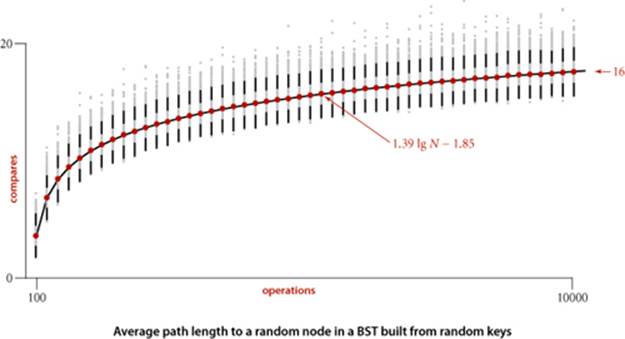
3.2.47 Average search time. Run empirical studies to compute the average and standard deviation of the average length of a path to a random node (internal path length divided by tree size, plus 1) in a BST built by insertion of N random keys into an initially empty tree, for N from 100 to 10,000. Do 1,000 trials for each tree size. Plot the results in a Tufte plot, like the one at the bottom of this page, fit with a curve plotting the function 1.39 lg N − 1.85 (see EXERCISE 3.2.35 and EXERCISE 3.2.39).
All materials on the site are licensed Creative Commons Attribution-Sharealike 3.0 Unported CC BY-SA 3.0 & GNU Free Documentation License (GFDL)
If you are the copyright holder of any material contained on our site and intend to remove it, please contact our site administrator for approval.
© 2016-2026 All site design rights belong to S.Y.A.