Algorithms (2014)
Three. Searching
3.3 Balanced Search Trees
The algorithms in the previous section work well for a wide variety of applications, but they have poor worst-case performance. We introduce in this section a type of binary search tree where costs are guaranteed to be logarithmic, no matter what sequence of keys is used to construct them. Ideally, we would like to keep our binary search trees perfectly balanced. In an N-node tree, we would like the height to be ~lg N so that we can guarantee that all searches can be completed in ~lg N compares, just as for binary search (see PROPOSITION B). Unfortunately, maintaining perfect balance for dynamic insertions is too expensive. In this section, we consider a data structure that slightly relaxes the perfect balance requirement to provide guaranteed logarithmic performance not just for the insert and search operations in our symbol-table API but also for all of the ordered operations (except range search).
2-3 search trees
The primary step to get the flexibility that we need to guarantee balance in search trees is to allow the nodes in our trees to hold more than one key. Specifically, referring to the nodes in a standard BST as 2-nodes (they hold two links and one key), we now also allow 3-nodes, which hold three links and two keys. Both 2-nodes and 3-nodes have one link for each of the intervals subtended by its keys.
Definition. A 2-3 search tree is a tree that is either empty or
• A 2-node, with one key (and associated value) and two links, a left link to a 2-3 search tree with smaller keys, and a right link to a 2-3 search tree with larger keys
• A 3-node, with two keys (and associated values) and three links, a left link to a 2-3 search tree with smaller keys, a middle link to a 2-3 search tree with keys between the node’s keys, and a right link to a 2-3 search tree with larger keys
As usual, we refer to a link to an empty tree as a null link.
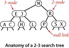
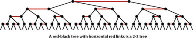
A perfectly balanced 2-3 search tree is one whose null links are all the same distance from the root. To be concise, we use the term 2-3 tree to refer to a perfectly balanced 2-3 search tree (the term denotes a more general structure in other contexts). Later, we shall see efficient ways to define and implement the basic operations on 2-nodes, 3-nodes, and 2-3 trees; for now, let us assume that we can manipulate them conveniently and see how we can use them as search trees.
Search
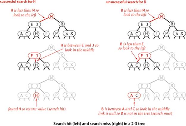
The search algorithm for keys in a 2-3 tree directly generalizes the search algorithm for BSTs. To determine whether a key is in the tree, we compare it against the keys at the root. If it is equal to any of them, we have a search hit; otherwise, we follow the link from the root to the subtree corresponding to the interval of key values that could contain the search key. If that link is null, we have a search miss; otherwise we recursively search in that subtree.
Insert into a 2-node
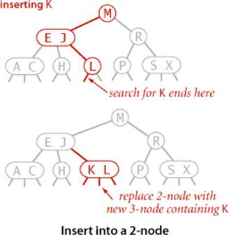
To insert a new key in a 2-3 tree, we might do an unsuccessful search and then hook on a new node with the key at the bottom, as we did with BSTs, but the new tree would not remain perfectly balanced. The primary reason that 2-3 trees are useful is that we can do insertions and still maintain perfect balance. It is easy to accomplish this task if the node at which the search terminates is a 2-node: we just replace the node with a 3-node containing its key and the new key to be inserted. If the node where the search terminates is a 3-node, we have more work to do.
Insert into a tree consisting of a single 3-node
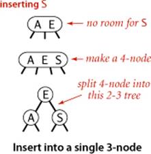
As a first warmup before considering the general case, suppose that we want to insert into a tiny 2-3 tree consisting of just a single 3-node. Such a tree has two keys, but no room for a new key in its one node. To be able to perform the insertion, we temporarily put the new key into a 4-node, a natural extension of our node type that has three keys and four links. Creating the 4-node is convenient because it is easy to convert it into a 2-3 tree made up of three 2-nodes, one with the middle key (at the root), one with the smallest of the three keys (pointed to by the left link of the root), and one with the largest of the three keys (pointed to by the right link of the root). Such a tree is a 3-node BST and also a perfectly balanced 2-3 search tree, with all the null links at the same distance from the root. Before the insertion, the height of the tree is 0; after the insertion, the height of the tree is 1. This case is simple, but it is worth considering because it illustrates height growth in 2-3 trees.
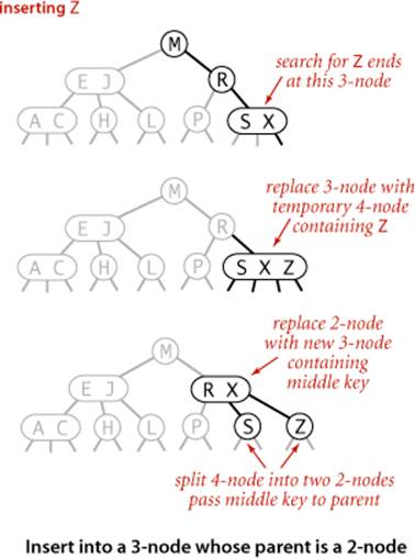
Insert into a 3-node whose parent is a 2-node
As a second warmup, suppose that the search ends at a 3-node at the bottom whose parent is a 2-node. In this case, we can still make room for the new key while maintaining perfect balance in the tree, by making a temporary 4-node as just described, then splitting the 4-node as just described, but then, instead of creating a new node to hold the middle key, moving the middle key to the node’s parent. You can think of the transformation as replacing the link to the old 3-node in the parent by the middle key with links on either side to the new 2-nodes. By our assumption, there is room for doing so in the parent: the parent was a 2-node (with one key and two links) and becomes a 3-node (with two keys and three links). Also, this transformation does not affect the defining properties of (perfectly balanced) 2-3 trees. The tree remains ordered because the middle key is moved to the parent, and it remains perfectly balanced: if all null links are the same distance from the root before the insertion, they are all the same distance from the root after the insertion. Be certain that you understand this transformation—it is the crux of 2-3 tree dynamics.
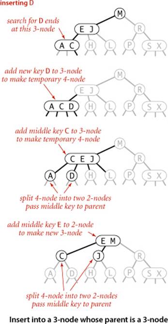
Insert into a 3-node whose parent is a 3-node
Now suppose that the search ends at a node whose parent is a 3-node. Again, we make a temporary 4-node as just described, then split it and insert its middle key into the parent. The parent was a 3-node, so we replace it with a temporary new 4-node containing the middle key from the 4-node split. Then, we perform precisely the same transformation on that node. That is, we split the new 4-node and insert its middle key into its parent. Extending to the general case is clear: we continue up the tree, splitting 4-nodes and inserting their middle keys in their parents until reaching a 2-node, which we replace with a 3-node that does not need to be further split, or until reaching a 3-node at the root.
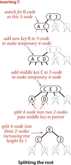
Splitting the root
If we have 3-nodes along the whole path from the insertion point to the root, we end up with a temporary 4-node at the root. In this case we can proceed in precisely the same way as for insertion into a tree consisting of a single 3-node. We split the temporary 4-node into three 2-nodes, increasing the height of the tree by 1. Note that this last transformation preserves perfect balance because it is performed at the root.
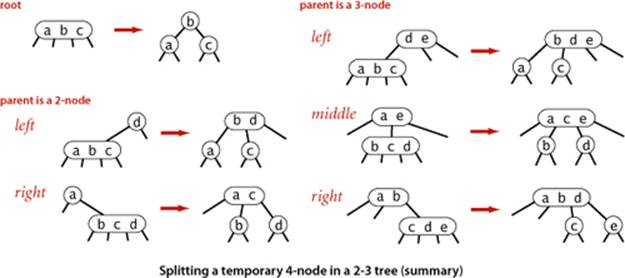
Local transformations
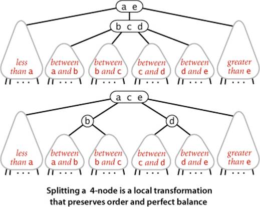
Splitting a temporary 4-node in a 2-3 tree involves one of six transformations, summarized at the bottom of the next page. The 4-node may be the root; it may be the left child or the right child of a 2-node; or it may be the left child, middle child, or right child of a 3-node. The basis of the 2-3 tree insertion algorithm is that all of these transformations are purely local: no part of the tree needs to be examined or modified other than the specified nodes and links. The number of links changed for each transformation is bounded by a small constant. In particular, the transformations are effective when we find the specified patterns anywhere in the tree, not just at the bottom. Each of the transformations passes up one of the keys from a 4-node to that node’s parent in the tree and then restructures links accordingly, without touching any other part of the tree.
Global properties
Moreover, these local transformations preserve the global properties that the tree is ordered and perfectly balanced: the number of links on the path from the root to any null link is the same. For reference, a complete diagram illustrating this point for the case that the 4-node is the middle child of a 3-node is shown above. If the length of every path from a root to a null link is h before the transformation, then it is h after the transformation. Each transformation preserves this property, even while splitting the 4-node into two 2-nodes and while changing the parent from a 2-node to a 3-node or from a 3-node into a temporary 4-node. When the root splits into three 2-nodes, the length of every path from the root to a null link increases by 1. If you are not fully convinced, work EXERCISE 3.3.7, which asks you to extend the diagrams at the top of the previous page for the other five cases to illustrate the same point. Understanding that every local transformation preserves order and perfect balance in the whole tree is the key to understanding the algorithm.
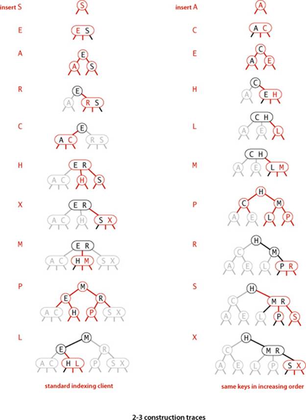
UNLIKE STANDARD BSTS, which grow down from the top, 2-3 trees grow up from the bottom. If you take the time to carefully study the figure on the next page, which gives the sequence of 2-3 trees that is produced by our standard indexing test client and the sequence of 2-3 trees that is produced when the same keys are inserted in increasing order, you will have a good understanding of the way that 2-3 trees are built. Recall that in a BST, the increasing-order sequence for 10 keys results in a worst-case tree of height 9. In the 2-3 trees, the height is 2.
The preceding description is sufficient to define a symbol-table implementation with 2-3 trees as the underlying data structure. Analyzing 2-3 trees is different from analyzing BSTs because our primary interest is in worst-case performance, as opposed to average-case performance (where we analyze expected performance under the random-key model). In symbol-table implementations, we normally have no control over the order in which clients insert keys into the table and worst-case analysis is one way to provide performance guarantees.
Proposition F. Search and insert operations in a 2-3 tree with N keys are guaranteed to visit at most lg N nodes.
Proof: The height of an N-node 2-3 tree is between ![]() log3 N
log3 N![]() =
= ![]() (lg N)/(lg 3)
(lg N)/(lg 3)![]() (if the tree is all 3-nodes) and
(if the tree is all 3-nodes) and ![]() lg N
lg N![]() (if the tree is all 2-nodes) (see EXERCISE 3.3.4).
(if the tree is all 2-nodes) (see EXERCISE 3.3.4).
Thus, we can guarantee good worst-case performance with 2-3 trees. The amount of time required at each node by each of the operations is bounded by a constant, and both operations examine nodes on just one path, so the total cost of any search or insert is guaranteed to be logarithmic. As you can see from comparing the 2-3 tree depicted at the bottom of page 431 with the BST formed from the same keys on page 405, a perfectly balanced 2-3 tree strikes a remarkably flat posture. For example, the height of a 2-3 tree that contains 1 billion keys is between 19 and 30. It is quite remarkable that we can guarantee to perform arbitrary search and insertion operations among 1 billion keys by examining at most 30 nodes.
However, we are only part of the way to an implementation. Although it is possible to write code that performs transformations on distinct data types representing 2- and 3-nodes, most of the tasks that we have described are inconvenient to implement in this direct representation because there are numerous different cases to be handled. We would need to maintain two different types of nodes, compare search keys against each of the keys in the nodes, copy links and other information from one type of node to another, convert nodes from one type to another, and so forth. Not only is there a substantial amount of code involved, but the overhead incurred could make the algorithms slower than standard BST search and insert. The primary purpose of balancing is to provide insurance against a bad worst case, but we would prefer the overhead cost for that insurance to be low. Fortunately, as you will see, we can do the transformations in a uniform way using little overhead.
Red-black BSTs
The insertion algorithm for 2-3 trees just described is not difficult to understand; now, we will see that it is also not difficult to implement. We will consider a simple representation known as a red-black BST that leads to a natural implementation. In the end, not much code is required, but understanding how and why the code gets the job done requires a careful look.
Encoding 3-nodes
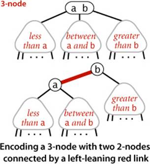
The basic idea behind red-black BSTs is to encode 2-3 trees by starting with standard BSTs (which are made up of 2-nodes) and adding extra information to encode 3-nodes. We think of the links as being of two different types: red links, which bind together two 2-nodes to represent 3-nodes, and black links, which bind together the 2-3 tree. Specifically, we represent 3-nodes as two 2-nodes connected by a single red link that leans left (one of the 2-nodes is the left child of the other). One advantage of using such a representation is that it allows us to use our get() code for standard BST search without modification. Given any 2-3 tree, we can immediately derive a corresponding BST, just by converting each node as specified. We refer to BSTs that represent 2-3 trees in this way as red-black BSTs.
An equivalent definition
Another way to proceed is to define red-black BSTs as BSTs having red and black links and satisfying the following three restrictions:
• Red links lean left.
• No node has two red links connected to it.
• The tree has perfect black balance: every path from the root to a null link has the same number of black links—we refer to this number as the tree’s black height.
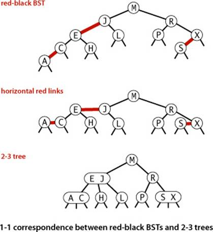
There is a 1-1 correspondence between red-black BSTs defined in this way and 2-3 trees.
A 1-1 correspondence
If we draw the red links horizontally in a red-black BST, all of the null links are the same distance from the root, and if we then collapse together the nodes connected by red links, the result is a 2-3 tree. Conversely, if we draw 3-nodes in a 2-3 tree as two 2-nodes connected by a red link that leans left, then no node has two red links connected to it, and the tree has perfect black balance, since the black links correspond to the 2-3 tree links, which are perfectly balanced by definition. Whichever way we choose to define them, red-black BSTs are both BSTs and 2-3 trees. Thus, if we can implement the 2-3 tree insertion algorithm by maintaining the 1-1 correspondence, then we get the best of both worlds: the simple and efficient search method from standard BSTs and the efficient insertion-balancing method from 2-3 trees.
Color representation
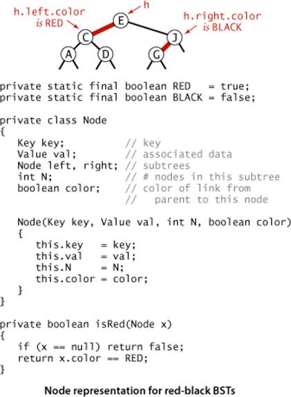
For convenience, since each node is pointed to by precisely one link (from its parent), we encode the color of links in nodes, by adding a boolean instance variable color to our Node data type, which is true if the link from the parent is red and false if it is black. By convention, null links are black. For clarity in our code, we define constants RED and BLACK for use in setting and testing this variable. We use a private method isRed() to test the color of a node’s link to its parent. When we refer to the color of a node, we are referring to the color of the link pointing to it, and vice versa.
Rotations
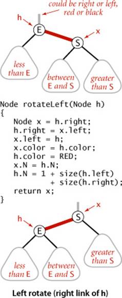
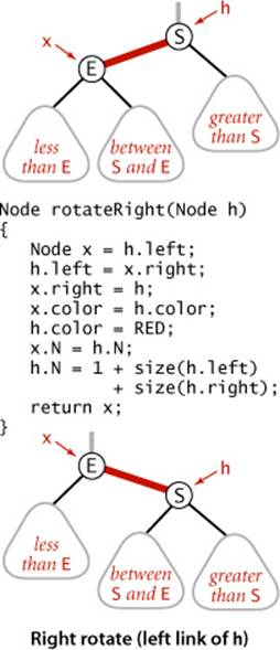
The implementation that we will consider might allow right-leaning red links or two red links in a row during an operation, but it always corrects these conditions before completion, through judicious use of an operation called rotation that switches the orientation of red links. First, suppose that we have a right-leaning red link that needs to be rotated to lean to the left (see the diagram at left). This operation is called a left rotation. We organize the computation as a method that takes a link to a red-black BST as argument and, assuming that link to be to a Node h whose right link is red, makes the necessary adjustments and returns a link to a node that is the root of a red-black BST for the same set of keys whose left link is red. If you check each of the lines of code against the before/after drawings in the diagram, you will find this operation is easy to understand: we are switching from having the smaller of the two keys at the root to having the larger of the two keys at the root. Implementing a right rotation that converts a left-leaning red link to a right-leaning one amounts to the same code, with left and right interchanged (see the diagram at right below).
Resetting the link in the parent after a rotation
Whether left or right, every rotation leaves us with a link. We always use the link returned by rotateRight() or rotateLeft() to reset the appropriate link in the parent (or the root of the tree). That may be a right or a left link, but we can always use it to reset the link in the parent. This link may be red or black—both rotateLeft() and rotateRight() preserve its color by setting x.color to h.color. This might allow two red links in a row to occur within the tree, but our algorithms will also use rotations to correct this condition when it arises. For example, the code
h = rotateLeft(h);
rotates left a right-leaning red link that is to the right of node h, setting h to point to the root of the resulting subtree (which contains all the same nodes as the subtree pointed to by h before the rotation, but a different root). The ease of writing this type of code is the primary reason we use recursive implementations of BST methods, as it makes doing rotations an easy supplement to normal insertion, as you will see.
WE CAN USE ROTATIONS to help maintain the 1-1 correspondence between 2-3 trees and red-black BSTs as new keys are inserted because they preserve the two defining properties of red-black BSTs: order and perfect black balance. That is, we can use rotations on a red-black BST without having to worry about losing its order or its perfect black balance. Next, we see how to use rotations to preserve the other two defining properties of red-black BSTs (no consecutive red links on any path and no right-leaning red links). We warm up with some easy cases.
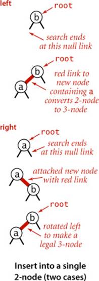
Insert into a single 2-node
A red-black BST with 1 key is just a single 2-node. Inserting the second key immediately shows the need for having a rotation operation. If the new key is smaller than the key in the tree, we just make a new (red) node with the new key and we are done: we have a red-black BST that is equivalent to a single 3-node. But if the new key is larger than the key in the tree, then attaching a new (red) node gives a right-leaning red link, and the code root = rotateLeft(root); completes the insertion by rotating the red link to the left and updating the tree root link. The result in both cases is the red-black representation of a single 3-node, with two keys, one left-leaning red link, and black height 0.
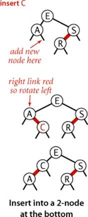
Insert into a 2-node at the bottom
We insert keys into a red-black BST as usual into a BST, adding a new node at the bottom (respecting the order), but always connected to its parent with a red link. If the parent is a 2-node, then the same two cases just discussed are effective. If the new node is attached to the left link, the parent simply becomes a 3-node; if it is attached to a right link, we have a 3-node leaning the wrong way, but a left rotation finishes the job.
Insert into a tree with two keys (in a 3-node)
This case reduces to three subcases: the new key is either less than both keys in the tree, between them, or greater than both of them. Each of the cases introduces a node with two red links connected to it; our goal is to correct this condition.
• The simplest of the three cases is when the new key is larger than the two in the tree and is therefore attached on the rightmost link of the 3-node, making a balanced tree with the middle key at the root, connected with red links to nodes containing a smaller and a larger key. If we flip the colors of those two links from red to black, then we have a balanced tree of (black) height 1 with three nodes, exactly what we need to maintain our 1-1 correspondence to 2-3 trees. The other two cases eventually reduce to this case.
• If the new key is smaller than the two keys in the tree and goes on the left link, then we have two red links in a row, both leaning to the left, which we can reduce to the previous case (middle key at the root, connected to the others by two red links) by rotating the top link to the right.
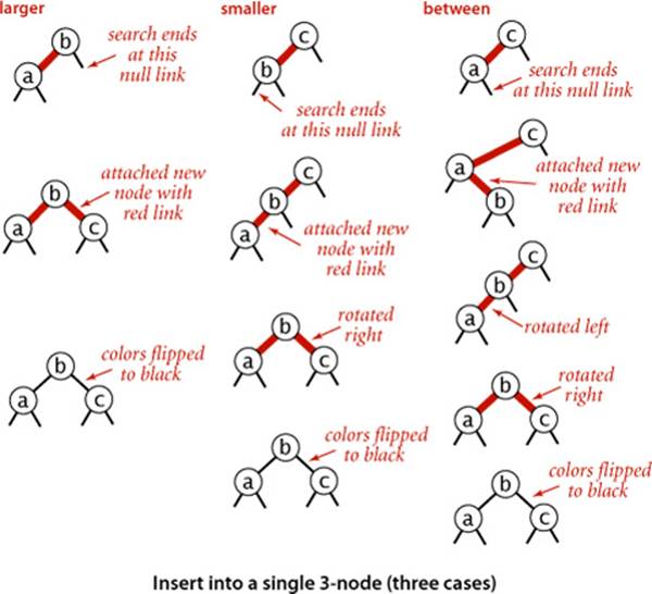
• If the new key goes between the two keys in the tree, we again have two red links in a row, a right-leaning one below a left-leaning one, which we can reduce to the previous case (two red links in a row, to the left) by rotating left the bottom link.
In summary, we achieve the desired result by doing zero, one, or two rotations followed by flipping the colors of the two children of the root. As with 2-3 trees, be certain that you understand these transformations, as they are the key to red-black tree dynamics.
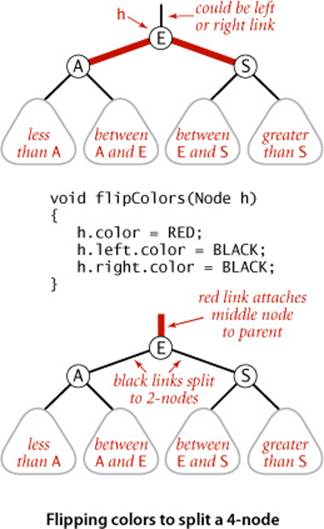
Flipping colors
To flip the colors of the two red children of a node, we use a method flipColors(), shown at left. In addition to flipping the colors of the children from red to black, we also flip the color of the parent from black to red. A critically important characteristic of this operation is that, like rotations, it is a local transformation that preserves perfect black balance in the tree. Moreover, this convention immediately leads us to a full implementation, as we describe next.
Keeping the root black
In the case just considered (insert into a single 3-node), the color flip will color the root red. This can also happen in larger trees. Strictly speaking, a red root implies that the root is part of a 3-node, but that is not the case, so we color the root black after each insertion. Note that the black height of the tree increases by 1 whenever the root is involved in a color flip, where its childrens’ colors are both flipped from red to black.
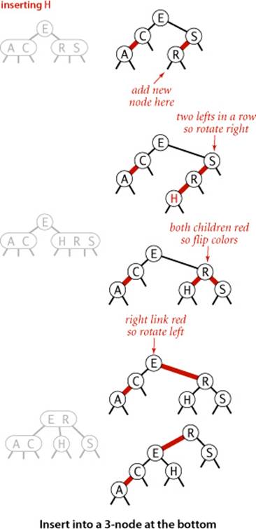
Insert into a 3-node at the bottom
Now suppose that we add a new node at the bottom that is connected to a 3-node. The same three cases just discussed arise. Either the new link is connected to the right link of the 3-node (in which case we just flip colors) or to the left link of the 3-node (in which case we need to rotate the top link right and flip colors) or to the middle link of the 3-node (in which case we rotate left the bottom link, then rotate right the top link, then flip colors). Flipping the colors makes the link to the middle node red, which amounts to passing it up to its parent, putting us back in the same situation with respect to the parent, which we can fix by moving up the tree.
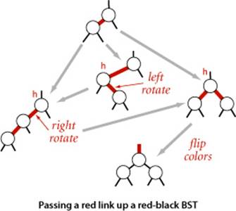
Passing a red link up the tree
The 2-3 tree insertion algorithm calls for us to split the 3-node, passing the middle key up to be inserted into its parent, continuing until encountering a 2-node or the root. In every case we have considered, we precisely accomplish this objective: after doing any necessary rotations, we flip colors, which turns the middle node to red. From the point of view of the parent of that node, that link becoming red can be handled in precisely the same manner as if the red link came from attaching a new node: we pass up a red link to the middle node. The three cases summarized in the diagram on the next page precisely capture the operations necessary in a red-black tree to implement the key operation in 2-3 tree insertion: to insert into a 3-node, create a temporary 4-node, split it, and pass a red link to the middle key up to its parent. Continuing the same process, we pass a red link up the tree until reaching a 2-node or the root.
IN SUMMARY, WE CAN MAINTAIN our 1-1 correspondence between 2-3 trees and red-black BSTs during insertion by judicious use of three simple operations: left rotate, right rotate, and color flip. We can accomplish the insertion by performing the following operations, one after the other, on each node as we pass up the tree from the point of insertion:
• If the right child is red and the left child is black, rotate left.
• If both the left child and its left child are red, rotate right.
• If both children are red, flip colors.
It certainly is worth your while to check that this sequence handles each of the cases just described. Note that the first operation handles both the rotation necessary to lean the 3-node to the left when the parent is a 2-node and the rotation necessary to lean the bottom link to the left when the new red link is the middle link in a 3-node.
Implementation
Since the balancing operations are to be performed on the way up the tree from the point of insertion, implementing them is easy in our standard recursive implementation: we just do them after the recursive calls, as shown in ALGORITHM 3.4. The three operations listed in the previous paragraph each can be accomplished with a single if statement that tests the colors of two nodes in the tree. Even though it involves a small amount of code, this implementation would be quite difficult to understand without the two layers of abstraction that we have developed (2-3 trees and red-black BSTs) to implement it. At a cost of testing three to five node colors (and perhaps doing a rotation or two or flipping colors when a test succeeds), we get BSTs that have nearly perfect balance.
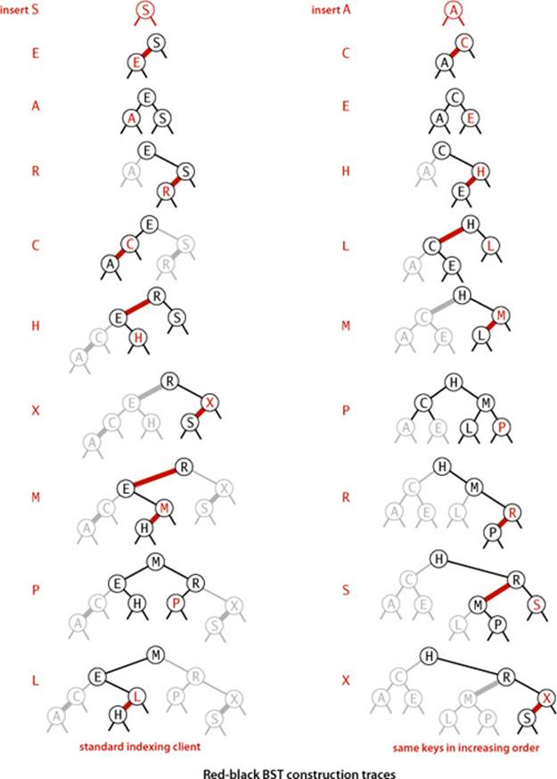
The traces for our standard indexing client and for the same keys inserted in increasing order are given on page 440. Considering these examples simply in terms of our three operations on red-black trees, as we have been doing, is an instructive exercise. Another instructive exercise is to check the correspondence with 2-3 trees that the algorithm maintains (using the figure for the same keys given on page 430). In both cases, you can test your understanding of the algorithm by considering the transformations (two color flips and two rotations) that are needed when P is inserted into the red-black BST (see EXERCISE 3.3.12).
Algorithm 3.4 Insert for red-black BSTs
public class RedBlackBST<Key extends Comparable<Key>, Value>
{
private Node root;
private class Node // BST node with color bit (see page 433)
private boolean isRed(Node h) // See page 433.
private Node rotateLeft(Node h) // See page 434.
private Node rotateRight(Node h) // See page 434.
private void flipColors(Node h) // See page 436.
private int size() // See page 398.
public void put(Key key, Value val)
{ // Search for key. Update value if found; grow table if new.
root = put(root, key, val);
root.color = BLACK;
}
private Node put(Node h, Key key, Value val)
{
if (h == null) // Do standard insert, with red link to parent.
return new Node(key, val, 1, RED);
int cmp = key.compareTo(h.key);
if (cmp < 0) h.left = put(h.left, key, val);
else if (cmp > 0) h.right = put(h.right, key, val);
else h.val = val;
if (isRed(h.right) && !isRed(h.left)) h = rotateLeft(h);
if (isRed(h.left) && isRed(h.left.left)) h = rotateRight(h);
if (isRed(h.left) && isRed(h.right)) flipColors(h);
h.N = size(h.left) + size(h.right) + 1;
return h;
}
}
The code for the recursive put() for red-black BSTs is identical to put() in elementary BSTs except for the three if statements after the recursive calls, which provide near-perfect balance in the tree by maintaining a 1-1 correspondence with 2-3 trees, on the way up the search path. The first rotates left any right-leaning 3-node (or a right-leaning red link at the bottom of a temporary 4-node); the second rotates right the top link in a temporary 4-node with two left-leaning red links; and the third flips colors to pass a red link up the tree (see text).
Deletion
Since put() in ALGORITHM 3.4 is already one of the most intricate methods that we consider in this book, and the implementations of deleteMin(), deleteMax(), and delete() for red-black BSTs are a bit more complicated, we defer their full implementations to exercises. Still, the basic approach is worthy of study. To describe it, we begin by returning to 2-3 trees. As with insertion, we can define a sequence of local transformations that allow us to delete a node while still maintaining perfect balance. The process is somewhat more complicated than for insertion, because we do the transformations both on the way down the search path, when we introduce temporary 4-nodes (to allow for a node to be deleted), and also on the way up the search path, where we split any leftover 4-nodes (in the same manner as for insertion).
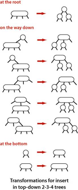
Top-down 2-3-4 trees
As a first warmup for deletion, we consider a simpler algorithm that does transformations both on the way down the path and on the way up the path: an insertion algorithm for 2-3-4 trees, where the temporary 4-nodes that we saw in 2-3 trees can persist in the tree. The insertion algorithm is based on doing transformations on the way down the path to maintain the invariant that the current node is not a 4-node (so we are assured that there will be room to insert the new key at the bottom) and transformations on the way up the path to balance any 4-nodes that may have been created. The transformations on the way down are precisely the same transformations that we used for splitting 4-nodes in 2-3 trees. If the root is a 4-node, we split it into three 2-nodes, increasing the height of the tree by 1. On the way down the tree, if we encounter a 4-node with a 2-node as parent, we split the 4-node into two 2-nodes and pass the middle key to the parent, making it a 3-node; if we encounter a 4-node with a 3-node as parent, we split the 4-node into two 2-nodes and pass the middle key to the parent, making it a 4-node. We do not need to worry about encountering a 4-node with a 4-node as parent by virtue of the invariant. At the bottom, we have, again by virtue of the invariant, a 2-node or a 3-node, so we have room to insert the new key. To implement this algorithm with red-black BSTs, we
• Represent 4-nodes as a balanced subtree of three 2-nodes, with both the left and right child connected to the parent with a red link
• Split 4-nodes on the way down the tree with color flips
• Balance 4-nodes on the way up the tree with rotations, as for insertion
Remarkably, you can implement top-down 2-3-4 trees by moving one line of code in put() in ALGORITHM 3.4: move the colorFlip() call (and accompanying test) to before the recursive calls (between the test for null and the comparison). This algorithm has some advantages over 2-3 trees in applications where multiple processes have access to the same tree, because it always is operating within a link or two of the current node. The deletion algorithms that we describe next are based on a similar scheme and are effective for these trees as well as for 2-3 trees.
Delete the minimum
As a second warmup for deletion, we consider the operation of deleting the minimum from a 2-3 tree. The basic idea is based on the observation that we can easily delete a key from a 3-node at the bottom of the tree, but not from a 2-node. Deleting the key from a 2-node leaves a node with no keys; the natural thing to do would be to replace the node with a null link, but that operation would violate the perfect balance condition. So, we adopt the following approach: to ensure that we do not end up on a 2-node, we perform appropriate transformations on the way down the tree to preserve the invariant that the current node is not a 2-node (it might be a 3-node or a temporary 4-node). First, at the root, there are two possibilities: if the root is a 2-node and both children are 2-nodes, we can just convert the three nodes to a 4-node; otherwise we can borrow from the right sibling if necessary to ensure that the left child of the root is not a 2-node. Then, on the way down the tree, one of the following cases must hold:
• If the left child of the current node is not a 2-node, there is nothing to do.
• If the left child is a 2-node and its immediate sibling is not a 2-node, move a key from the sibling to the left child.
• If the left child and its immediate sibling are 2-nodes, then combine them with the smallest key in the parent to make a 4-node, changing the parent from a 3-node to a 2-node or from a 4-node to a 3-node.
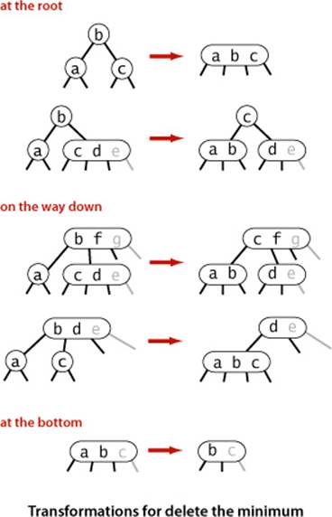
Following this process as we traverse left links to the bottom, we wind up on a 3-node or a 4-node with the smallest key, so we can just remove it, converting the 3-node to a 2-node or the 4-node to a 3-node. Then, on the way up the tree, we split any unused temporary 4-nodes.
Delete
The same transformations along the search path just described for deleting the minimum are effective to ensure that the current node is not a 2-node during a search for any key. If the search key is at the bottom, we can just remove it. If the key is not at the bottom, then we have to exchange it with its successor as in regular BSTs. Then, since the current node is not a 2-node, we have reduced the problem to deleting the minimum in a subtree whose root is not a 2-node, and we can use the procedure just described for that subtree. After the deletion, as usual, we split any remaining 4-nodes on the search path on the way up the tree.
SEVERAL OF THE EXERCISES at the end of this section are devoted to examples and implementations related to these deletion algorithms. People with an interest in developing or understanding implementations need to master the details covered in these exercises. People with a general interest in the study of algorithms need to recognize that these methods are important because they represent the first symbol-table implementation that we have seen where search, insert, and delete are all guaranteed to be efficient, as we will establish next.
Properties of red-black BSTs
Studying the properties of red-black BSTs is a matter of checking the correspondence with 2-3 trees and then applying the analysis of 2-3 trees. The end result is that all symbol-table operations in red-black BSTs are guaranteed to be logarithmic in the size of the tree (except for range search, which additionally costs time proportional to the number of keys returned). We repeat and emphasize this point because of its importance.
Analysis
First, we establish that red-black BSTs, while not perfectly balanced, are always nearly so, regardless of the order in which the keys are inserted. This fact immediately follows from the 1-1 correspondence with 2-3 trees and the defining property of 2-3 trees (perfect balance).
Proposition G. The height of a red-black BST with N nodes is no more than 2 lg N.
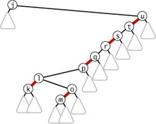
Proof sketch: The worst case is a 2-3 tree that is all 2-nodes except that the leftmost path is made up of 3-nodes. The path taking left links from the root is twice as long as the paths of length ~ lg N that involve just 2-nodes. It is possible, but not easy, to develop key sequences that cause the construction of red-black BSTs whose average path length is the worst-case 2 lg N. If you are mathematically inclined, you might enjoy exploring this issue by working EXERCISE 3.3.24.
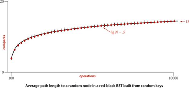
This upper bound is conservative: experiments involving both random insertions and insertion sequences found in typical applications support the hypothesis that each search in a red-black BST of N nodes uses about 1.0 lg N − .5 compares, on the average. Moreover, you are not likely to encounter a substantially higher average number of compares in practice.
Property H. The average length of a path from the root to a node in a red-black BST with N nodes is ~1.00 lg N.
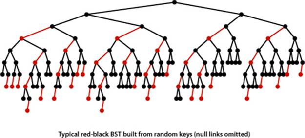
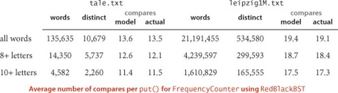
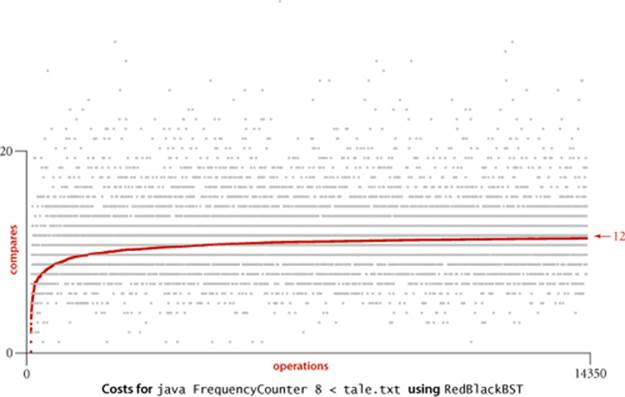
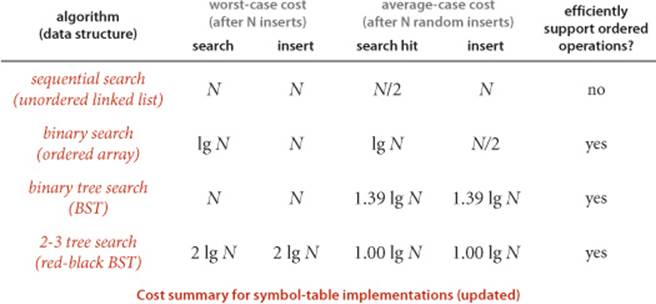
Evidence: Typical trees, such as the one at the bottom of the previous page (and even the one built by inserting keys in increasing order at the bottom of this page) are quite well-balanced, by comparison with typical BSTs (such as the tree depicted on page 405). The table at the top of this page shows that path lengths (search costs) for our FrequencyCounter application are about 40 percent lower than from elementary BSTs, as expected. This performance has been observed in countless applications and experiments since the invention of red-black BSTs.
For our example study of the cost of the put() operations for FrequencyCounter for words of length 8 or more, we see a further reduction in the average cost, again providing a quick validation of the logarithmic performance predicted by the theoretical model, though this validation is less surprising than for BSTs because of the guarantee provided by PROPOSITION G. The total savings is less than the 40 per cent savings in the search cost because we count rotations and color flips as well as compares.
The get() method in red-black BSTs does not examine the node color, so the balancing mechanism adds no overhead; search is faster than in elementary BSTs because the tree is balanced. Each key is inserted just once, but may be involved in many, many search operations, so the end result is that we get search times that are close to optimal (because the trees are nearly balanced and no work for balancing is done during the searches) at relatively little cost (unlike binary search, insertions are guaranteed to be logarithmic). The inner loop of the search is a compare followed by updating a link, which is quite short, like the inner loop of binary search (compare and index arithmetic). This implementation is the first we have seen with logarithmic guarantees for both search and insert, and it has a tight inner loop, so its use is justified in a broad variety of applications, including library implementations.
Ordered symbol-table API
One of the most appealing features of red-black BSTs is that the complicated code is limited to the put() (and deletion) methods. Our code for the minimum/maximum, select, rank, floor, ceiling and range queries in standard BSTs can be used without any change, since it operates on BSTs and has no need to refer to the node color. ALGORITHM 3.4, together with these methods (and the deletion methods), leads to a complete implementation of our ordered symbol-table API. Moreover, all of the methods benefit from the near-perfect balance in the tree because they all require time proportional to the tree height, at most. Thus PROPOSITION G, in combination with PROPOSITION E, suffices to establish a logarithmic performance guarantee for all of them.
Proposition I. In a red-black BST, the following operations take logarithmic time in the worst case: search, insertion, finding the minimum, finding the maximum, floor, ceiling, rank, select, delete the minimum, delete the maximum, delete, and range count.
Proof: We have just discussed get(), put(), and the deletion operations. For the others, the code from SECTION 3.2 can be used verbatim (it just ignores the node color). Guaranteed logarithmic performance follows from PROPOSITIONS E and G, and the fact that each algorithm performs a constant number of operations on each node examined.
On reflection, it is quite remarkable that we are able to achieve such guarantees. In a world awash with information, where people maintain tables with trillions or quadrillions of entries, the fact is that we can guarantee to complete any one of these operations in such tables with just a few dozen compares.
Q&A
Q. Why not let the 3-nodes lean either way and also allow 4-nodes in the trees?
A. Those are fine alternatives, used by many for decades. You can learn about several of these alternatives in the exercises. The left-leaning convention reduces the number of cases and therefore requires substantially less code.
Q. Why not use an array of Key values to represent 2-, 3-, and 4-nodes with a single Node type?
A. Good question. That is precisely what we do for B-trees (see CHAPTER 6), where we allow many more keys per node. For the small nodes in 2-3 trees, the overhead for the array is too high a price to pay.
Q. When we split a 4-node, we sometimes set the color of the right node to RED in rotateRight() and then immediately set it to BLACK in flipColors(). Isn’t that wasteful?
A. Yes, and we also sometimes unnecessarily recolor the middle node. In the grand scheme of things, resetting a few extra bits is not in the same league with the improvement from linear to logarithmic that we get for all operations, but in performance-critical applications, you can put the code for rotateRight() and flipColors() inline and eliminate those extra tests. We use those methods for deletion, as well, and find them slightly easier to use, understand, and maintain by making sure that they preserve perfect black balance.
Exercises
3.3.1 Draw the 2-3 tree that results when you insert the keys E A S Y Q U T I O N in that order into an initially empty tree.
3.3.2 Draw the 2-3 tree that results when you insert the keys Y L P M X H C R A E S in that order into an initially empty tree.
3.3.3 Find an insertion order for the keys S E A R C H X M that leads to a 2-3 tree of height 1.
3.3.4 Prove that the height of a 2-3 tree with N keys is between ~ log3 N ≈ .63 lg N (for a tree that is all 3-nodes) and ~lg N (for a tree that is all 2-nodes).
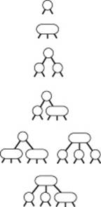
3.3.5 The figure at right shows all the structurally different 2-3 trees with N keys, for N from 1 up to 6 (ignore the order of the subtrees). Draw all the structurally different trees for N = 7, 8, 9, and 10.
3.3.6 Find the probability that each of the 2-3 trees in EXERCISE 3.3.5 is the result of the insertion of N random distinct keys into an initially empty tree.
3.3.7 Draw diagrams like the one at the top of page 428 for the other five cases in the diagram at the bottom of that page.
3.3.8 Show all possible ways that one might represent a 4-node with three 2-nodes bound together with red links (not necessarily left-leaning).
3.3.9 Which of the following are red-black BSTs?
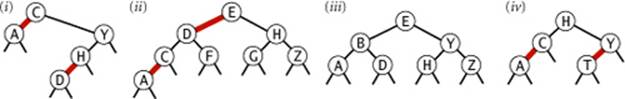
3.3.10 Draw the red-black BST that results when you insert items with the keys E A S Y Q U T I O N in that order into an initially empty tree.
3.3.11 Draw the red-black BST that results when you insert items with the keys Y L P M X H C R A E S in that order into an initially empty tree.
3.3.12 Draw the red-black BST that results after each transformation (color flip or rotation) during the insertion of P for our standard indexing client.
3.3.13 True or false: If you insert keys in increasing order into a red-black BST, the tree height is monotonically increasing.
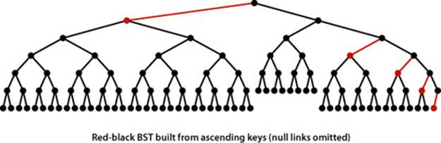
3.3.14 Draw the red-black BST that results when you insert letters A through K in order into an initially empty tree, then describe what happens in general when trees are built by insertion of keys in ascending order (see also the figure in the text).
3.3.15 Answer the previous two questions for the case when the keys are inserted in descending order.
3.3.16 Show the result of inserting n into the red-black BST drawn at right (only the search path is shown, and you need to include only these nodes in your answer).
3.3.17 Generate two random 16-node red-black BSTs. Draw them (either by hand or with a program). Compare them with the (unbalanced) BSTs built with the same keys.
3.3.18 Draw all the structurally different red-black BSTs with N keys, for N from 2 up to 10 (see EXERCISE 3.3.5).
3.3.19 With 1 bit per node for color, we can represent 2-, 3-, and 4-nodes. How many bits per node would we need to represent 5-, 6-, 7-, and 8-nodes with a binary tree?
3.3.20 Compute the internal path length in a perfectly balanced BST of N nodes, when N is a power of 2 minus 1.
3.3.21 Create a test client for RedBlackBST, based on your solution to EXERCISE 3.2.10.
3.3.22 Find a sequence of keys to insert into a BST and into a red-black BST such that the height of the BST is less than the height of the red-black BST, or prove that no such sequence is possible.
Creative Problems
3.3.23 2-3 trees without balance restriction. Develop an implementation of the basic symbol-table API that uses 2-3 trees that are not necessarily balanced as the underlying data structure. Allow 3-nodes to lean either way. Hook the new node onto the bottom with a black link when inserting into a 3-node at the bottom. Run experiments to develop a hypothesis estimating the average path length in a tree built from N random insertions.
3.3.24 Worst case for red-black BSTs. Show how to construct a red-black BST demonstrating that, in the worst case, almost all the paths from the root to a null link in a red-black BST of N nodes are of length 2 lg N.
3.3.25 Top-down 2-3-4 trees. Develop an implementation of the basic symbol-table API that uses balanced 2-3-4 trees as the underlying data structure, using the red-black representation and the insertion method described in the text, where 4-nodes are split by flipping colors on the way down the search path and balancing on the way up.
3.3.26 Single top-down pass. Develop a modified version of your solution to EXERCISE 3.3.25 that does not use recursion. Complete all the work splitting and balancing 4-nodes (and balancing 3-nodes) on the way down the tree, finishing with an insertion at the bottom.
3.3.27 Allow right-leaning red links. Develop a modified version of your solution to EXERCISE 3.3.25 that allows right-leaning red links in the tree.
3.3.28 Bottom-up 2-3-4 trees. Develop an implementation of the basic symbol-table API that uses balanced 2-3-4 trees as the underlying data structure, using the red-black representation and a bottom-up insertion method based on the same recursive approach as ALGORITHM 3.4. Your insertion method should split only the sequence of 4-nodes (if any) on the bottom of the search path.
3.3.29 Optimal storage. Modify RedBlackBST so that it does not use any extra storage for the color bit, based on the following trick: To color a node red, swap its two links. Then, to test whether a node is red, test whether its left child is larger than its right child. You have to modify the compares to accommodate the possible link swap, and this trick replaces bit compares with key compares that are presumably more expensive, but it shows that the bit in the nodes can be eliminated, if necessary.
3.3.30 Sofware caching. Modify RedBlackBST to keep the most recently accessed Node in an instance variable so that it can be accessed in constant time if the next put() or get() uses the same key (see EXERCISE 3.1.25).
3.3.31 Tree drawing. Add a method draw() to RedBlackBST that draws red-black BST figures in the style of the text (see EXERCISE 3.2.38)
3.3.32 AVL trees. An AVL tree is a BST where the height of every node and that of its sibling differ by at most 1. (The oldest balanced tree algorithms are based on using rotations to maintain height balance in AVL trees.) Show that coloring red links that go from nodes of even height to nodes of odd height in an AVL tree gives a (perfectly balanced) 2-3-4 tree, where red links are not necessarily left-leaning. Extra credit: Develop an implementation of the symbol-table API that uses this as the underlying data structure. One approach is to keep a height field in each node, using rotations after the recursive calls to adjust the height as necessary; another is to use the red-black representation and use methods like moveRedLeft() and moveRedRight() in EXERCISE 3.3.39 and EXERCISE 3.3.40.
3.3.33 Certification. Add to RedBlackBST a method is23() to check that no node is connected to two red links and that there are no right-leaning red links and a method isBalanced() to check that all paths from the root to a null link have the same number of black links. Combine these methods with code from isBST() in EXERCISE 3.2.31 to create a method isRedBlackBST() that checks that the tree is a red-black BST.
3.3.34 All 2-3 trees. Write code to generate all structurally different 2-3 trees of height 2, 3, and 4. There are 2, 7, and 122 such trees, respectively. (Hint: Use a symbol table.)
3.3.35 2-3 trees. Write a program TwoThreeST.java that uses two node types to implement 2-3 search trees directly.
3.3.36 2-3-4-5-6-7-8 trees. Describe algorithms for search and insertion in balanced 2-3-4-5-6-7-8 search trees.
3.3.37 Memoryless. Show that red-black BSTs are not memoryless: for example, if you insert a key that is smaller than all the keys in the tree and then immediately delete the minimum, you may get a different tree.
3.3.38 Fundamental theorem of rotations. Show that any BST can be transformed into any other BST on the same set of keys by a sequence of left and right rotations.
3.3.39 Delete the minimum. Implement the deleteMin() operation for red-black BSTs by maintaining the correspondence with the transformations given in the text for moving down the left spine of the tree while maintaining the invariant that the current node is not a 2-node.
Solution:
private Node moveRedLeft(Node h)
{ // Assuming that h is red and both h.left and h.left.left
// are black, make h.left or one of its children red.
flipColors(h);
if (isRed(h.right.left))
{
h.right = rotateRight(h.right);
h = rotateLeft(h);
}
return h;
}
public void deleteMin()
{
if (!isRed(root.left) && !isRed(root.right))
root.color = RED;
root = deleteMin(root);
if (!isEmpty()) root.color = BLACK;
}
private Node deleteMin(Node h)
{
if (h.left == null)
return null;
if (!isRed(h.left) && !isRed(h.left.left))
h = moveRedLeft(h);
h.left = deleteMin(h.left);
return balance(h);
}
This code assumes a balance() method that consists of the line of code
if (isRed(h.right)) h = rotateLeft(h);
followed by the last five lines of the recursive put() in ALGORITHM 3.4 and a flipColors() implementation that complements the three colors, instead of the method given in the text for insertion. For deletion, we set the parent to BLACK and the two children to RED.
3.3.40 Delete the maximum. Implement the deleteMax() operation for red-black BSTs. Note that the transformations involved differ slightly from those in the previous exercise because red links are left-leaning.
Solution:
private Node moveRedRight(Node h)
{ // Assuming that h is red and both h.right and h.right.left
// are black, make h.right or one of its children red.
flipColors(h)
if (isRed(h.left.left))
h = rotateRight(h);
return h;
}
public void deleteMax()
{
if (!isRed(root.left) && !isRed(root.right))
root.color = RED;
root = deleteMax(root);
if (!isEmpty()) root.color = BLACK;
}
private Node deleteMax(Node h)
{
if (isRed(h.left))
h = rotateRight(h);
if (h.right == null)
return null;
if (!isRed(h.right) && !isRed(h.right.left))
h = moveRedRight(h);
h.right = deleteMax(h.right);
return balance(h);
}
3.3.41 Delete. Implement the delete() operation for red-black BSTs, combining the methods of the previous two exercises with the delete() operation for BSTs.
Solution:
public void delete(Key key)
{
if (!isRed(root.left) && !isRed(root.right))
root.color = RED;
root = delete(root, key);
if (!isEmpty()) root.color = BLACK;
}
private Node delete(Node h, Key key)
{
if (key.compareTo(h.key) < 0)
{
if (!isRed(h.left) && !isRed(h.left.left))
h = moveRedLeft(h);
h.left = delete(h.left, key);
}
else
{
if (isRed(h.left))
h = rotateRight(h);
if (key.compareTo(h.key) == 0 && (h.right == null))
return null;
if (!isRed(h.right) && !isRed(h.right.left))
h = moveRedRight(h);
if (key.compareTo(h.key) == 0)
{
Node x = min(h.right);
h.key = x.key;
h.val = x.val;z
h.right = deleteMin(h.right);
}
else h.right = delete(h.right, key);
}
return balance(h);
}
Experiments
3.3.42 Count red nodes. Write a program that computes the percentage of red nodes in a given red-black BST. Test your program by running at least 100 trials of the experiment of inserting N random keys into an initially empty tree, for N = 104, 105, and 106, and formulate an hypothesis.
3.3.43 Cost plots. Instrument RedBlackBST so that you can produce plots like the ones in this section showing the cost of each put() operation during the computation (see EXERCISE 3.1.38).
3.3.44 Average search time. Run empirical studies to compute the average and standard deviation of the average length of a path to a random node (internal path length divided by tree size plus 1) in a red-black BST built by insertion of N random keys into an initially empty tree, for N from 1 to 10,000. Do at least 1,000 trials for each tree size. Plot the results in a Tufte plot, like the one at the bottom of this page, fit with a curve plotting the function lg N − .5.
3.3.45 Count rotations. Instrument your program for EXERCISE 3.3.43 to plot the number of rotations and node splits that are used to build the trees. Discuss the results.
3.3.46 Height. Instrument your program for EXERCISE 3.3.43 to plot the height of red-black BSTs. Discuss the results.
All materials on the site are licensed Creative Commons Attribution-Sharealike 3.0 Unported CC BY-SA 3.0 & GNU Free Documentation License (GFDL)
If you are the copyright holder of any material contained on our site and intend to remove it, please contact our site administrator for approval.
© 2016-2026 All site design rights belong to S.Y.A.