Algorithms (2014)
One. Fundamentals
1.4 Analysis of Algorithms
AS PEOPLE GAIN EXPERIENCE USING COMPUTERS, they use them to solve difficult problems or to process large amounts of data and are invariably led to questions like these:
How long will my program take?
Why does my program run out of memory?
You certainly have asked yourself these questions, perhaps when rebuilding a music or photo library, installing a new application, working with a large document, or working with a large amount of experimental data. The questions are much too vague to be answered precisely—the answers depend on many factors such as properties of the particular computer being used, the particular data being processed, and the particular program that is doing the job (which implements some algorithm). All of these factors leave us with a daunting amount of information to analyze.
Despite these challenges, the path to developing useful answers to these basic questions is often remarkably straightforward, as you will see in this section. This process is based on the scientific method, the commonly accepted body of techniques used by scientists to develop knowledge about the natural world. We apply mathematical analysis to develop concise models of costs and do experimental studies to validate these models.
Scientific method
The very same approach that scientists use to understand the natural world is effective for studying the running time of programs:
• Observe some feature of the natural world, generally with precise measurements.
• Hypothesize a model that is consistent with the observations.
• Predict events using the hypothesis.
• Verify the predictions by making further observations.
• Validate by repeating until the hypothesis and observations agree.
One of the key tenets of the scientific method is that the experiments we design must be reproducible, so that others can convince themselves of the validity of the hypothesis. Hypotheses must also be falsifiable, so that we can know for sure when a given hypothesis is wrong (and thus needs revision). As Einstein famously is reported to have said (“No amount of experimentation can ever prove me right; a single experiment can prove me wrong”), we can never know for sure that any hypothesis is absolutely correct; we can only validate that it is consistent with our observations.
Observations
Our first challenge is to determine how to make quantitative measurements of the running time of our programs. This task is far easier than in the natural sciences. We do not have to send a rocket to Mars or kill laboratory animals or split an atom—we can simply run the program. Indeed,every time you run a program, you are performing a scientific experiment that relates the program to the natural world and answers one of our core questions: How long will my program take?
Our first qualitative observation about most programs is that there is a problem size that characterizes the difficulty of the computational task. Normally, the problem size is either the size of the input or the value of a command-line argument. Intuitively, the running time should increase with problem size, but the question of by how much it increases naturally comes up every time we develop and run a program.
Another qualitative observation for many programs is that the running time is relatively insensitive to the input itself; it depends primarily on the problem size. If this relationship does not hold, we need to take steps to better understand and perhaps better control the running time’s sensitivity to the input. But it does often hold, so we now focus on the goal of better quantifying the relationship between problem size and running time.
Example
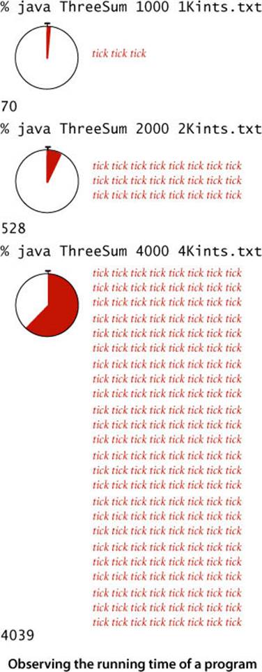
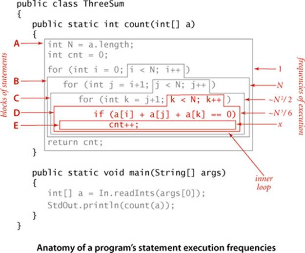
As a running example, we will work with the program ThreeSum shown here, which counts the number of triples in a file of N integers that sum to 0 (assuming that overflow plays no role). This computation may seem contrived to you, but it is deeply related to numerous fundamental computational tasks (for example, see EXERCISE 1.4.26). As a test input, consider the file 1Mints.txt from the booksite, which contains 1 million randomly generated int values. The second, eighth, and tenth entries in 1Mints.txt sum to 0. How many more such triples are there in the file? ThreeSum can tell us, but can it do so in a reasonable amount of time? What is the relationship between the problem size N and running time for ThreeSum? As a first experiment, try running ThreeSum on your computer for the files 1Kints.txt, 2Kints.txt, 4Kints.txt, and 8Kints.txt on the booksite that contain the first 1,000, 2,000, 4,000, and 8,000 integers from 1Mints.txt, respectively. You can quickly determine that there are 70 triples that sum to 0 in 1Kints.txt and that there are 528 triples that sum to 0 in 2Kints.txt. The program takes substantially more time to determine that there are 4,039 triples that sum to 0 in 4Kints.txt, and as you wait for the program to finish for 8Kints.txt, you will find yourself asking the question How long will my program take? As you will see, answering this question for this program turns out to be easy. Indeed, you can often come up with a fairly accurate prediction while the program is running.
Given N, how long will this program take?
public class ThreeSum
{
public static int count(int[] a)
{ // Count triples that sum to 0.
int N = a.length;
int cnt = 0;
for (int i = 0; i < N; i++)
for (int j = i+1; j < N; j++)
for (int k = j+1; k < N; k++)
if (a[i] + a[j] + a[k] == 0)
cnt++;
return cnt;
}
public static void main(String[] args)
{
int[] a = In.readInts(args[0]);
StdOut.println(count(a));
}
}
% more 1Mints.txt
324110
-442472
626686
-157678
508681
123414
-77867
155091
129801
287381
604242
686904
-247109
77867
982455
-210707
-922943
-738817
85168
855430
...
Stopwatch
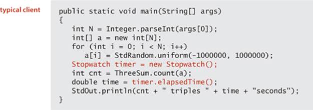
Reliably measuring the exact running time of a given program can be difficult. Fortunately, we are usually happy with estimates. We want to be able to distinguish programs that will finish in a few seconds or a few minutes from those that might require a few days or a few months or more, and we want to know when one program is twice as fast as another for the same task. Still, we need accurate measurements to generate experimental data that we can use to formulate and to check the validity of hypotheses about the relationship between running time and problem size. For this purpose, we use the Stopwatch data type shown on the facing page. Its elapsedTime() method returns the elapsed time since it was created, in seconds. The implementation is based on using the Java system’s currentTimeMillis() method, which gives the current time in milliseconds, to save the time when the constructor is invoked, then uses it again to compute the elapsed time when elapsedTime() is invoked.
Analysis of experimental data
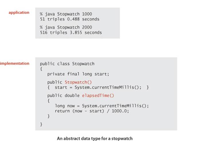
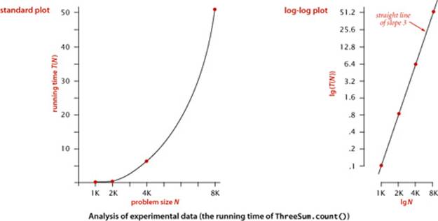
The program DoublingTest on the facing page is a more sophisticated Stopwatch client that produces experimental data for ThreeSum. It generates a sequence of random input arrays, doubling the array size at each step, and prints the running times of ThreeSum.count() for each input size. These experiments are certainly reproducible—you can also run them on your own computer, as many times as you like. When you run DoublingTest, you will find yourself in a prediction-verification cycle: it prints several lines very quickly, but then slows down considerably. Each time it prints a line, you find yourself wondering how long it will be until it prints the next line. Of course, since you have a different computer from ours, the actual running times that you get are likely to be different from those shown for our computer. Indeed, if your computer is twice as fast as ours, your running times will be about half ours, which leads immediately to the well-founded hypothesis that running times on different computers are likely to differ by a constant factor. Still, you will find yourself asking the more detailed question How long will my program take, as a function of the input size? To help answer this question, we plot the data. The diagrams at the bottom of the facing page show the result of plotting the data, both on a normal and on a log-log scale, with the problem size N on the x-axis and the running time T(N) on the y-axis. The log-log plot immediately leads to a hypothesis about the running time—the data fits a straight line of slope 3 on the log-log plot. The equation of such a line is
lg(T(N)) = 3 lg N + lg a
(where a is a constant) which is equivalent to
T(N) = aN3
the running time, as a function of the input size, as desired. We can use one of our data points to solve for a—for example, T(8000) = 51.1 = a80003, so a = 9.98×10⁻¹¹—and then use the equation
T(N) = 9.98×10⁻¹¹N3
to predict running times for large N. Informally, we are checking the hypothesis that the data points on the log-log plot fall close to this line. Statistical methods are available for doing a more careful analysis to find estimates of a and the exponent b, but our quick calculations suffice to estimate running time for most purposes. For example, we can estimate the running time on our computer for N = 16,000 to be about 9.98×10−11160003 = 408.8 seconds, or about 6.8 minutes (the actual time was 409.3 seconds). While waiting for your computer to print the line for N = 16,000 in DoublingTest, you might use this method to predict when it will finish, then check the result by waiting to see if your prediction is true.
So far, this process mirrors the process scientists use when trying to understand properties of the real world. A straight line in a log-log plot is equivalent to the hypothesis that the data fits the equation T(N) = aNb. Such a fit is known as a power law. A great many natural and synthetic phenomena are described by power laws, and it is reasonable to hypothesize that the running time of a program does, as well. Indeed, for the analysis of algorithms, we have mathematical models that strongly support this and similar hypotheses, to which we now turn.
Mathematical models
In the early days of computer science, D. E. Knuth postulated that, despite all of the complicating factors in understanding the running times of our programs, it is possible, in principle, to build a mathematical model to describe the running time of any program. Knuth’s basic insight is simple: the total running time of a program is determined by two primary factors:
• The cost of executing each statement
• The frequency of execution of each statement
The former is a property of the computer, the Java compiler and the operating system; the latter is a property of the program and the input. If we know both for all instructions in the program, we can multiply them together and sum for all instructions in the program to get the running time.
The primary challenge is to determine the frequency of execution of the statements. Some statements are easy to analyze: for example, the statement that sets cnt to 0 in ThreeSum.count() is executed exactly once. Others require higher-level reasoning: for example, the if statement in ThreeSum.count()is executed precisely
N(N−1)(N−2)/6
times (the number of ways to pick three different numbers from the input array—see EXERCISE 1.4.1). Others depend on the input data: for example the number of times the instruction cnt++ in ThreeSum.count() is executed is precisely the number of triples that sum to 0 in the input, which could range from 0 of them to all of them. In the case of DoublingTest, where we generate the numbers randomly, it is possible to do a probabilistic analysis to determine the expected value of this quantity (see EXERCISE 1.4.40).
Tilde approximations
Frequency analyses of this sort can lead to complicated and lengthy mathematical expressions. For example, consider the count just considered of the number of times the if statement in ThreeSum is executed:
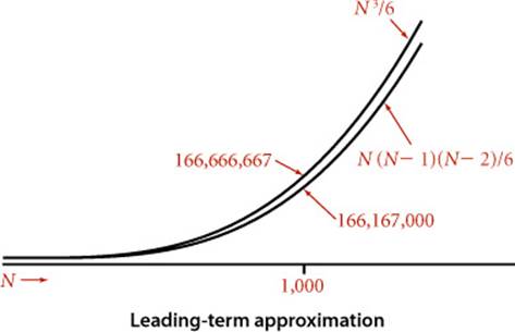
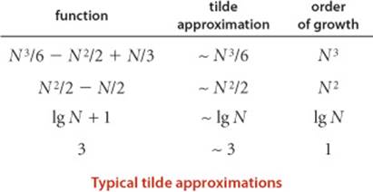
N(N−1)(N−2)/6 = N3/6 − N2/2 + N/3
As is typical in such expressions, the terms after the leading term are relatively small (for example, when N = 1,000 the value of − N2/2 + N/3 ≈ −499,667 is certainly insignificant by comparison with N3/6 ≈ 166,666,667). To allow us to ignore insignificant terms and therefore substantially simplify the mathematical formulas that we work with, we often use a mathematical device known as the tilde notation (~). This notation allows us to work with tilde approximations, where we throw away low-order terms that complicate formulas and represent a negligible contribution to values of interest:
Definition. We write ~f(N) to represent any function that, when divided by f(N), approaches 1 as N grows, and we write g(N) ~ f(N) to indicate that g(N)/f(N) approaches 1 as N grows.
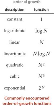
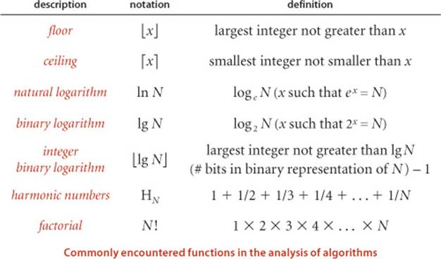
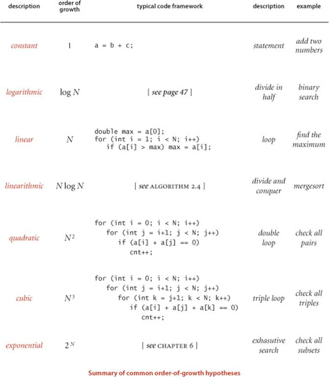
For example, we use the approximation ~N3/6 to describe the number of times the if statement in ThreeSum is executed, since N3/6 − N2/2 + N/3 divided by N3/6 approaches 1 as N grows. Most often, we work with tilde approximations of the form g(N) ~ a f(N) where f(N) = Nb(log N)c with a, b, and c constants and refer to f(N) as the order of growth of g(N). When using the logarithm in the order of growth, we generally do not specify the base, since the constant a can absorb that detail. This usage covers the relatively few functions that are commonly encountered in studying the order of growth of a program’s running time shown in the table at left (with the exception of the exponential, which we defer to CONTEXT). We will describe these functions in more detail and briefly discuss why they appear in the analysis of algorithms after we complete our treatment ofThreeSum.
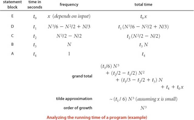
Approximate running time
To follow through on Knuth’s approach to develop a mathematical expression for the total running time of a Java program, we can (in principle) study our Java compiler to find the number of machine instructions corresponding to each Java instruction and study our machine specifications to find the time of execution of each of the machine instructions, to produce a grand total. This process, for ThreeSum, is briefly summarized on the facing page. We classify blocks of Java statements by their frequency of execution, develop leading-term approximations for the frequencies, determine the cost of each statement, and then compute a total. Note that some frequencies may depend on the input. In this case, the number of times cnt++ is executed certainly depends on the input—it is the number of triples that sum to 0, and could range from 0 to ~N3/6. We stop short of exhibiting the details (values of the constants) for any particular system, except to highlight that by using constant values t0, t1, t2, ... for the time taken by the blocks of statements, we are assuming that each block of Java statements corresponds to machine instructions that require a specified fixed amount of time. A key observation from this exercise is to note that only the instructions that are executed the most frequently play a role in the final total—we refer to these instructions as the inner loop of the program. For ThreeSum, the inner loop is the statements that increment k and test that it is less than N and the statements that test whether the sum of three given numbers is 0 (and possibly the statement that implements the count, depending on the input). This behavior is typical: the running times of a great many programs depend only on a small subset of their instructions.
Order-of-growth hypothesis
In summary, the experiments on page 177 and the mathematical model on page 181 both support the following hypothesis:
Property A. The order of growth of the running time of ThreeSum (to compute the number of triples that sum to 0 among N numbers) is N3.
Evidence: Let T(N) be the running time of ThreeSum for N numbers. The mathematical model just described suggests that T(N) ~ aN3 for some machine-dependent constant a; experiments on many computers (including yours and ours) validate that approximation.
Throughout this book, we use the term property to refer to a hypothesis that needs to be validated through experimentation. The end result of our mathematical analysis is precisely the same as the end result of our experimental analysis—the running time of ThreeSum is ~ aN3 for a machine-dependent constant a. This match validates both the experiments and the mathematical model and also exhibits more insight about the program because it does not require experimentation to determine the exponent. With some effort, we could validate the value of a on a particular system as well, though that activity is generally reserved for experts in situations where performance is critical.
Analysis of algorithms
Hypotheses such as PROPERTY A are significant because they relate the abstract world of a Java program to the real world of a computer running it. Working with the order of growth allows us to take one further step: to separate a program from the algorithm it implements. The idea that the order of growth of the running time of ThreeSum is N3 does not depend on the fact that it is implemented in Java or that it is running on your laptop or someone else’s cellphone or a supercomputer; it depends primarily on the fact that it examines all the different triples of numbers in the input. The algorithm that you are using (and sometimes the input model) determines the order of growth. Separating the algorithm from the implementation on a particular computer is a powerful concept because it allows us to develop knowledge about the performance of algorithms and then apply that knowledge to any computer. For example, we might say that ThreeSum is an implementation of the brute-force algorithm “compute the sum of all different triples, counting those that sum to 0”—we expect that an implementation of this algorithm in any programming language on any computer will lead to a running time that is proportional to N3. In fact, much of the knowledge about the performance of classic algorithms was developed decades ago, but that knowledge is still relevant to today’s computers.
3-sum cost model. When studying algorithms to solve the 3-sum problem, we count array accesses (the number of times an array entry is accessed, for read or write).
Cost model
We focus attention on properties of algorithms by articulating a cost model that defines the basic operations used by the algorithms we are studying to solve the problem at hand. For example, an appropriate cost model for the 3-sum problem, shown at right, is the number of times we access an array entry. With this cost model, we can make precise mathematical statements about properties of an algorithm, not just a particular implementation, as follows:
Proposition B. The brute-force 3-sum algorithm uses ~N3/2 array accesses to compute the number of triples that sum to 0 among N numbers.
Proof: The algorithm accesses each of the 3 numbers for each of the ~N3/6 triples.
We use the term proposition to refer to mathematical truths about algorithms in terms of a cost model. Throughout this book, we study the algorithms that we consider within the framework of a specific cost model. Our intent is to articulate cost models such that the order of growth of the running time for a given implementation is the same as the order of growth of the cost of the underlying algorithm (in other words, the cost model should include operations that fall within the inner loop). We seek precise mathematical results about algorithms (propositions) and also hypotheses about performance of implementations (properties) that you can check through experimentation. In this case, PROPOSITION B is a mathematical truth that supports the hypothesis stated in PROPERTY A, which we have validated with experiments, in accordance with the scientific method.
Summary
For many programs, developing a mathematical model of running time reduces to the following steps:
• Develop an input model, including a definition of the problem size.
• Identify the inner loop.
• Define a cost model that includes operations in the inner loop.
• Determine the frequency of execution of those operations for the given input. Doing so might require mathematical analysis—we will consider some examples in the context of specific fundamental algorithms later in the book.
If a program is defined in terms of multiple methods, we normally consider the methods separately. As an example, consider our example program of SECTION 1.1, BinarySearch.
Binary search. The input model is the array a[] of size N; the inner loop is the statements in the single while loop; the cost model is the compare operation (compare the values of two array entries); and the analysis, discussed in SECTION 1.1 and given in full detail in PROPOSITION B in SECTION 3.1, shows that the number of compares is at most lg N + 1.
Whitelist. The input model is the N numbers in the whitelist and the M numbers on standard input where we assume M >> N; the inner loop is the statements in the single while loop; the cost model is the compare operation (inherited from binary search); and the analysis is immediate given the analysis of binary search—the number of compares is at most M (lg N + 1).
Thus, we draw the conclusion that the order of growth of the running time of the whitelist computation is at most M lg N, subject to the following considerations:
• If N is small, the input-output cost might dominate.
• The number of compares depends on the input—it lies between ~M and ~M lgN, depending on how many of the numbers on standard input are in the whitelist and on how long the binary search takes to find the ones that are (typically it is ~M lgN).
• We are assuming that the cost of Arrays.sort() is small compared to M lg N. Arrays.sort() implements the mergesort algorithm, and in SECTION 2.2, we will see that the order of growth of the running time of mergesort is N log N (see PROPOSITION G in CHAPTER 2), so this assumption is justified.
Thus, the model supports our hypothesis from SECTION 1.1 that the binary search algorithm makes the computation feasible when M and N are large. If we double the length of the standard input stream, then we can expect the running time to double; if we double the size of the whitelist, then we can expect the running time to increase only slightly.
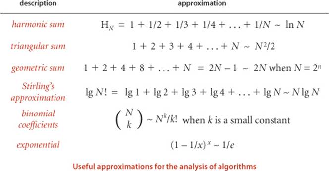
DEVELOPING MATHEMATICAL MODELS for the analysis of algorithms is a fruitful area of research that is somewhat beyond the scope of this book. Still, as you will see with binary search, mergesort, and many other algorithms, understanding certain mathematical models is critical to understanding the efficiency of fundamental algorithms, so we often present details and/or quote the results of classic studies. When doing so, we encounter various functions and approximations that are widely used in mathematical analysis. For reference, we summarize some of this information in the tables below.
Order-of-growth classifications
We use just a few structural primitives (statements, conditionals, loops, nesting, and method calls) to implement algorithms, so very often the order of growth of the cost is one of just a few functions of the problem size N. These functions are summarized in the table on the facing page, along with the names that we use to refer to them, typical code that leads to each function, and examples.
Constant
A program whose running time’s order of growth is constant executes a fixed number of operations to finish its job; consequently its running time does not depend on N. Most Java operations take constant time.
Logarithmic
A program whose running time’s order of growth is logarithmic is barely slower than a constant-time program. The classic example of a program whose running time is logarithmic in the problem size is binary search (see BinarySearch on page 47). The base of the logarithm is not relevant with respect to the order of growth (since all logarithms with a constant base are related by a constant factor), so we use log N when referring to order of growth.
Linear
Programs that spend a constant amount of time processing each piece of input data, or that are based on a single for loop, are quite common. The order of growth of such a program is said to be linear—its running time is proportional to N.
Linearithmic
We use the term linearithmic to describe programs whose running time for a problem of size N has order of growth N log N. Again, the base of the logarithm is not relevant with respect to the order of growth. The prototypical examples of linearithmic algorithms are Merge.sort() (see ALGORITHM 2.4) and Quick.sort() (see ALGORITHM 2.5).
Quadratic
A typical program whose running time has order of growth N2 has two nested for loops, used for some calculation involving all pairs of N elements. The elementary sorting algorithms Selection.sort() (see ALGORITHM 2.1) and Insertion.sort() (see ALGORITHM 2.2) are prototypes of the programs in this classification.
Cubic
A typical program whose running time has order of growth N3 has three nested for loops, used for some calculation involving all triples of N elements. Our example for this section, ThreeSum, is a prototype.
Exponential
In CHAPTER 6 (but not until then!) we will consider programs whose running times are proportional to 2N or higher. Generally, we use the term exponential to refer to algorithms whose order of growth is bN for any constant b > 1, even though different values of b lead to vastly different running times. Exponential algorithms are extremely slow—you will never run one of them to completion for a large problem. Still, exponential algorithms play a critical role in the theory of algorithms because there exists a large class of problems for which it seems that an exponential algorithm is the best possible choice.
THESE CLASSIFICATIONS ARE THE MOST COMMON, but certainly not a complete set. The order of growth of an algorithm’s cost might be N2logN or N3/2 or some similar function. Indeed, the detailed analysis of algorithms can require the full gamut of mathematical tools that have been developed over the centuries.
A great many of the algorithms that we consider have straightforward performance characteristics that can be accurately described by one of the orders of growth that we have considered. Accordingly, we can usually work with specific propositions with a cost model, such as mergesort uses between ½Nlg N and NlgN compares that immediately imply hypotheses (properties) such as the order of growth of mergesort’s running time is linearithmic. For economy, we abbreviate such a statement to just say mergesort is linearithmic.
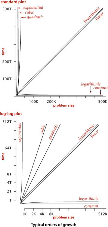
The plots at left indicate the importance of the order of growth in practice. The x-axis is the problem size; the y-axis is the running time. These charts make plain that quadratic and cubic algorithms are not feasible for use on large problems. As it turns out, several important problems have natural solutions that are quadratic but clever algorithms that are linearithmic. Such algorithms (including mergesort) are critically important in practice because they enable us to address problem sizes far larger than could be addressed with quadratic solutions. Naturally, we therefore focus in this book on developing logarithmic, linear, and linearithmic algorithms for fundamental problems.
Designing faster algorithms
One of the primary reasons to study the order of growth of a program is to help design a faster algorithm to solve the same problem. To illustrate this point, we consider next a faster algorithm for the 3-sum problem. How can we devise a faster algorithm, before even embarking on the study of algorithms? The answer to this question is that we have discussed and used two classic algorithms, mergesort and binary search, have introduced the facts that the mergesort is linearithmic and binary search is logarithmic. How can we take advantage of these algorithms to solve the 3-sum problem?
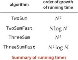
Warmup: 2-sum
Consider the easier problem of determining the number of pairs of integers in an input file that sum to 0. To simplify the discussion, assume also that the integers are distinct. This problem is easily solved in quadratic time by deleting the k loop and a[k] from ThreeSum.count(), leaving a double loop that examines all pairs, as shown in the quadratic entry in the table on page 187 (we refer to such an implementation as TwoSum). The implementation below shows how mergesort and binary search (see page 47) can serve as a basis for a linearithmic solution to the 2-sum problem. The improved algorithm is based on the fact that an entry a[i] is one of a pair that sums to 0 if and only if the value -a[i] is in the array (and a[i] is not zero). To solve the problem, we sort the array (to enable binary search) and then, for every entry a[i] in the array, do a binary search for -a[i] withrank() in BinarySearch. If the result is an index j with j > i, we increment the count. This succinct test covers three cases:
• An unsuccessful binary search returns -1, so we do not increment the count.
• If the binary search returns j > i, we have a[i] + a[j] = 0, so we increment the count.
• If the binary search returns j between 0 and i, we also have a[i] + a[j] = 0 but do not increment the count, to avoid double counting.
Linearithmic solution to the 2-sum problem
import java.util.Arrays;
public class TwoSumFast
{
public static int count(int[] a)
{ // Count pairs that sum to 0.
Arrays.sort(a);
int N = a.length;
int cnt = 0;
for (int i = 0; i < N; i++)
if (BinarySearch.rank(-a[i], a) > i)
cnt++;
return cnt;
}
public static void main(String[] args)
{
int[] a = In.readInts(args[0]);
StdOut.println(count(a));
}
}
The result of the computation is precisely the same as the result of the quadratic algorithm, but it takes much less time. The running time of the mergesort is proportional to N log N, and the N binary searches each take time proportional to log N, so the running time of the whole algorithm is proportional to N log N. Developing a faster algorithm like this is not merely an academic exercise—the faster algorithm enables us to address much larger problems. For example, you are likely to be able to solve the 2-sum problem for 1 million integers (1Mints.txt) in a reasonable amount of time on your computer, but you would have to wait quite a long time to do it with the quadratic algorithm (see EXERCISE 1.4.41).
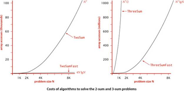
Fast algorithm for 3-sum
The very same idea is effective for the 3-sum problem. Again, assume also that the integers are distinct. A pair a[i] and a[j] is part of a triple that sums to 0 if and only if the value -(a[i] + a[j]) is in the array (and not a[i] or a[j]). The code below sorts the array, then does N(N−1)/2 binary searches that each take time proportional to log N, for a total running time proportional to N2 log N. Note that in this case the cost of the sort is insignificant. Again, this solution enables us to address much larger problems (see EXERCISE 1.4.42). The plots in the figure at the bottom of the next page show the disparity in costs among these four algorithms for problem sizes in the range we have considered. Such differences certainly motivate the search for faster algorithms.
Lower bounds
The table on page 191 summarizes the discussion of this section. An interesting question immediately arises: Can we find algorithms for the 2-sum and 3-sum problems that are substantially faster than TwoSumFast and ThreeSumFast? Is there a linear algorithm for 2-sum or a linearithmic algorithm for 3-sum? The answer to this question is no for 2-sum (under a model that counts and allows only comparisons of linear or quadratic functions of the numbers) and no one knows for 3-sum, though experts believe that the best possible algorithm for 3-sum is quadratic. The idea of a lower bound on the order of growth of the worst-case running time for all possible algorithms to solve a problem is a very powerful one, which we will revisit in detail in SECTION 2.2 in the context of sorting. Nontrivial lower bounds are difficult to establish, but very helpful in guiding our search for efficient algorithms.
N2 lg N solution to the 3-sum problem
import java.util.Arrays;
public class ThreeSumFast
{
public static int count(int[] a)
{ // Count triples that sum to 0.
Arrays.sort(a);
int N = a.length;
int cnt = 0;
for (int i = 0; i < N; i++)
for (int j = i+1; j < N; j++)
if (BinarySearch.rank(-a[i]-a[j], a) > j)
cnt++;
return cnt;
}
public static void main(String[] args)
{
int[] a = In.readInts(args[0]);
StdOut.println(count(a));
}
}
THE EXAMPLES IN THIS SECTION SET THE STAGE for our treatment of algorithms in this book. Throughout the book, our strategy for addressing new problems is the following:
• Implement and analyze a straighforward solution to the problem. We usually refer to such solutions, like ThreeSum and TwoSum, as the brute-force solution.
• Examine algorithmic improvements, usually designed to reduce the order of growth of the running time, such as TwoSumFast and ThreeSumFast.
• Run experiments to validate the hypotheses that the new algorithms are faster.
In many cases, we examine several algorithms for the same problem, because running time is only one consideration when choosing an algorithm for a practical problem. We will develop this idea in detail in the context of fundamental problems throughout the book.
Doubling ratio experiments
The following is a simple and effective shortcut for predicting performance and for determining the approximate order of growth of the running time of any program:
• Develop an input generator that produces inputs that model the inputs expected in practice (such as the random integers in timeTrial() in DoublingTest.)
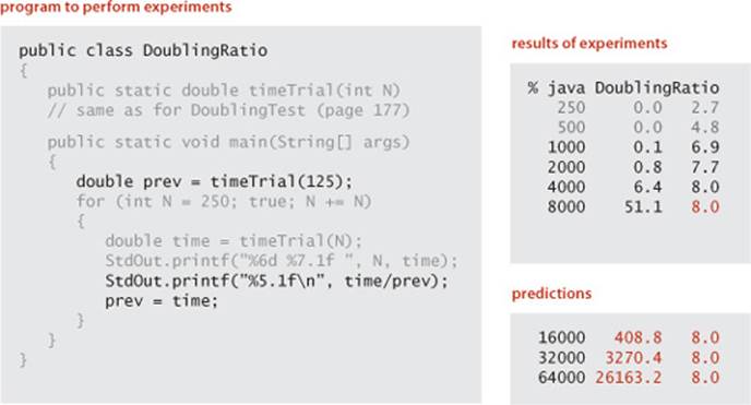
• Run the program DoublingRatio given below, a modification of DoublingTest that calculates the ratio of each running time with the previous.
• Run until the ratios approach a limit 2b.
This test is not effective if the ratios do not approach a limiting value, but they do for many, many programs, implying the following conclusions:
• The order of growth of the running time is approximately Nb.
• To predict running times, multiply the last observed running time by 2b and double N, continuing as long as desired. If you want to predict for an input size that is not a power of 2 times N, you can adjust ratios accordingly (see EXERCISE 1.4.9).
As illustrated below, the ratio for ThreeSum is about 8 and we can predict the running times for N = 16,000, 32,000, 64,000 to be 408.8, 3270.4, 26163.2 seconds, respectively, just by successively multiplying the last time for 8,000 (51.1) by 8.
This test is roughly equivalent to the process described on page 176 (run experiments, plot values on a log-log plot to develop the hypothesis that the running time is aNb, determine the value of b from the slope of the line, then solve for a), but it is simpler to apply. Indeed, you can accurately predict preformance by hand when you run DoublingRatio. As the ratio approaches a limit, just multiply by that ratio to fill in later values in the table. Your approximate model of the order of growth is a power law with the binary logarithm of that ratio as the power.
Why does the ratio approach a constant? A simple mathematical calculation shows that to be the case for all of the common orders of growth just discussed (except exponential):
Proposition C. (Doubling ratio) If T(N) ~ aNblgN then T(2N)/T(N) ~ 2b.
Proof: Immediate from the following calculation:
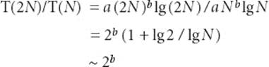
Generally, the logarithmic factor cannot be ignored when developing a mathematical model, but it plays a less important role in predicting performance with a doubling hypothesis.
YOU SHOULD CONSIDER running doubling ratio experiments for every program that you write where performance matters—doing so is a very simple way to estimate the order of growth of the running time, perhaps revealing a performance bug where a program may turn out to be not as efficient as you might think. More generally, we can use hypotheses about the order of growth of the running time of programs to predict performance in one of the following ways:
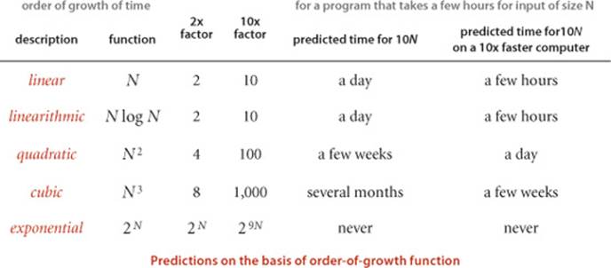
Estimating the feasibility of solving large problems
You need to be able to answer this basic question for every program that you write: Will the program be able to process this given input data in a reasonable amount of time? To address such questions for a large amount of data, we extrapolate by a much larger factor than for doubling, say 10, as shown in the fourth column in the table at the bottom of the next page. Whether it is an investment banker running daily financial models or a scientist running a program to analyze experimental data or an engineer running simulations to test a design, it is not unusual for people to regularly run programs that take several hours to complete, so the table focuses on that situation. Knowing the order of growth of the running time of an algorithm provides precisely the information that you need to understand limitations on the size of the problems that you can solve.Developing such understanding is the most important reason to study performance. Without it, you are likely have no idea how much time a program will consume; with it, you can make a back-of-the-envelope calculation to estimate costs and proceed accordingly.
Estimating the value of using a faster computer
You also may be faced with this basic question, periodically: How much faster can I solve the problem if I get a faster computer? Generally, if the new computer is x times faster than the old one, you can improve your running time by a factor of x. But it is usually the case that you can address larger problems with your new computer. How will that change affect the running time? Again, the order of growth is precisely the information needed to answer that question.
A FAMOUS RULE OF THUMB known as Moore’s Law implies that you can expect to have a computer with about double the speed and double the memory 18 months from now, or a computer with about 10 times the speed and 10 times the memory in about 5 years. The table below demonstrates that an algorithm cannot keep pace with Moore’s Law (solving a problem that is twice as big with a computer that is twice as fast) if its running time is quadratic or cubic. You can quickly determine whether that is the case by doing a doubling ratio test and checking that the ratio of running times as the input size doubles approaches 2 (linear or linearithmic), not 4 (quadratic) or 8 (cubic).
Caveats
There are many reasons that you might get inconsistent or misleading results when trying to analyze program performance in detail. All of them have to do with the idea that one or more of the basic assumptions underlying our hypotheses might be not quite correct. We can develop new hypotheses based on new assumptions, but the more details that we need to take into account, the more care is required in the analysis.
Large constants
With leading-term approximations, we ignore constant coefficients in lower-order terms, which may not be justifed. For example, when we approximate the function 2N2 + c N by ~2N2, we are assuming that c is small. If that is not the case (suppose that c is 103 or 106) the approximation is misleading. Thus, we have to be sensitive to the possibility of large constants.
Nondominant inner loop
The assumption that the inner loop dominates may not always be correct. The cost model might miss the true inner loop, or the problem size N might not be sufficiently large to make the leading term in the mathematical description of the frequency of execution of instructions in the inner loop so much larger than lower-order terms that we can ignore them. Some programs have a significant amount of code outside the inner loop that needs to be taken into consideration. In other words, the cost model may need to be refined.
Instruction time
The assumption that each instruction always takes the same amount of time is not always correct. For example, most modern computer systems use a technique known as caching to organize memory, in which case accessing elements in huge arrays can take much longer if they are not close together in the array. You might observe the effect of caching for ThreeSum by letting DoublingRatio run for a while. After seeming to converge to 8, the ratio of running times may jump to a larger value for large arrays because of caching.
System considerations
Typically, there are many, many things going on in your computer. Java is one application of many competing for resources, and Java itself has many options and controls that significantly affect performance. A garbage collector or a just-in-time compiler or a download from the internet might drastically affect the results of experiments. Such considerations can interfere with the bedrock principle of the scientific method that experiments should be reproducible, since what is happening at this moment in your computer will never be reproduced again. Whatever else is going on in your system should in principle be negligible or possible to control.
Too close to call
Often, when we compare two different programs for the same task, one might be faster in some situations, and slower in others. One or more of the considerations just mentioned could make the difference. There is a natural tendency among some programmers (and some students) to devote an extreme amount of energy running races to find the “best” implementation, but such work is best left for experts.
Strong dependence on inputs
One of the first assumptions that we made in order to determine the order of growth of the program’s running time of a program was that the running time should be relatively insensitive to the inputs. When that is not the case, we may get inconsistent results or be unable to validate our hypotheses. For example, suppose that we modify ThreeSum to answer the question Does the input have a triple that sums to 0 ? by changing it to return a boolean value, replacing cnt++ by return true and adding return false as the last statement. The order of growth of the running time of this program is constant if the first three integers sum to 0 and cubic if there are no such triples in the input.
Multiple problem parameters
We have been focusing on measuring performance as a function of a single parameter, generally the value of a command-line argument or the size of the input. However, it is not unusual to have several parameters. A typical example arises when an algorithm involves building a data structure and then performing a sequence of operations that use that data structure. Both the size of the data structure and the number of operations are parameters for such applications. We have already seen an example of this in our analysis of the problem of whitelisting using binary search, where we have N numbers in the whitelist and M numbers on standard input and a typical running time proportional to M logN.
Despite all these caveats, understanding the order of growth of the running time of each program is valuable knowledge for any programmer, and the methods that we have described are powerful and broadly applicable. Knuth’s insight was that we can carry these methods through to the last detail in principle to make detailed, accurate predictions. Typical computer systems are extremely complex and close analysis is best left for experts, but the same methods are effective for developing approximate estimates of the running time of any program. A rocket scientist needs to have some idea of whether a test flight will land in the ocean or in a city; a medical researcher needs to know whether a drug trial will kill or cure all the subjects; and any scientist or engineer using a computer program needs to have some idea of whether it will run for a second or for a year.
Coping with dependence on inputs
For many problems, one of the most significant of the caveats just mentioned is the dependence on inputs, because running times can vary widely. The running time of the modification of ThreeSum mentioned on the facing page ranges from constant to cubic, depending on the input, so a closer analysis is required if we want to predict performance. We briefly consider here some of the approaches that are effective and that we will consider for specific algorithms later in the book.
Input models
One approach is to more carefully model the kind of input to be processed in the problems that we need to solve. For example, we might assume that the numbers in the input to ThreeSum are random int values. This approach is challenging for two reasons:
• The model may be unrealistic.
• The analysis may be extremely difficult, requiring mathematical skills quite beyond those of the typical student or programmer.
The first of these is the more significant, often because the goal of a computation is to discover characteristics of the input. For example, if we are writing a program to process a genome, how can we estimate its performance on a different genome? A good model describing the genomes found in nature is precisely what scientists seek, so estimating the running time of our programs on data found in nature actually amounts to contributing to that model! The second challenge leads to a focus on mathematical results only for our most important algorithms. We will see several examples where a simple and tractable input model, in conjunction with classical mathematical analysis, helps us predict performance.
Worst-case performance guarantees
Some applications demand that the running time of a program be less than a certain bound, no matter what the input. To provide such performance guarantees, theoreticians take an extremely pessimistic view of the performance of algorithms: what would the running time be in the worst case? For example, such a conservative approach might be appropriate for the software that runs a nuclear reactor or a pacemaker or the brakes in your car. We want to guarantee that such software completes its job within the bounds that we set because the result could be catastrophic if it does not. Scientists normally do not contemplate the worst case when studying the natural world: in biology, the worst case might be the extinction of the human race; in physics, the worst case might be the end of the universe. But the worst case can be a very real concern in computer systems, where the input may be generated by another (potentially malicious) user, rather than by nature. For example, websites that do not use algorithms with performance guarantees are subject to denial-of-service attacks, where hackers flood them with pathological requests that make them run much more slowly than planned. Accordingly, many of our algorithms are designed to provide performance guarantees, such as the following:
Proposition D. In the linked-list implementations of Bag (ALGORITHM 1.4), Stack (ALGORITHM 1.2), and Queue (ALGORITHM 1.3), all operations take constant time in the worst case.
Proof: Immediate from the code. The number of instructions executed for each operation is bounded by a small constant. Caveat: This argument depends upon the (reasonable) assumption that the Java system creates a new Node in constant time.
Randomized algorithms
One important way to provide a performance guarantee is to introduce randomness. For example, the quicksort algorithm for sorting that we study in SECTION 2.3 (perhaps the most widely used sorting algorithm) is quadratic in the worst case, but randomly ordering the input gives a probabilistic guarantee that its running time is linearithmic. Every time you run the algorithm, it will take a different amount of time, but the chance that the time will not be linearithmic is so small as to be negligible. Similarly, the hashing algorithms for symbol tables that we study in SECTION 3.4 (again, perhaps the most widely used approach) are linear-time in the worst case, but constant-time under a probabilistic guarantee. These guarantees are not absolute, but the chance that they are invalid is less than the chance your computer will be struck by lightning. Thus, such guarantees are as useful in practice as worst-case guarantees.
Sequences of operations
For many applications, the algorithm “input” might be not just data, but the sequence of operations performed by the client. For example, a pushdown stack where the client pushes N values, then pops them all, may have quite different performance characteristics from one where the client issues an alternating sequence N of push and pop operations. Our analysis has to take both situations into account (or to include a reasonable model of the sequence of operations).
Amortized analysis
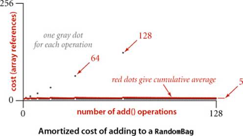
Accordingly, another way to provide a performance guarantee is to amortize the cost, by keeping track of the total cost of all operations, divided by the number of operations. In this setting, we can allow some expensive operations, while keeping the average cost of operations low. The prototypical example of this type of analysis is the study of the resizing array data structure for Stack that we considered in SECTION 1.3 (ALGORITHM 1.1 on page 141). For simplicity, suppose that N is a power of 2. Starting with an empty structure, how many array entries are accessed for Nconsecutive calls to push()? This quantity is easy to calculate: the number of array accesses is
N + 4 + 8 + 16 + ... + 2N = 5N − 4
The first term accounts for the array access within each of the N calls to push(); the subsequent terms account for the array accesses to initialize the data structure each time it doubles in size. Thus the average number of array accesses per operation is constant, even though the last operation takes linear time. This is known as an “amortized” analysis because we spread the cost of the few expensive operations, by assigning a portion of it to each of a large number of inexpensive operations. Amortized analysis provides a worst case guarantee on any sequence of operations, starting from an empty data structure. VisualAccumulator illustrates the process, shown above.
Proposition E. In the resizing array implementation of Stack (ALGORITHM 1.1), the average number of array accesses for any sequence of push and pop operations starting from an empty data structure is constant in the worst case.
Proof sketch: For each push operation that causes the array to grow (say from size N to size 2N), consider the N/2 – 1 push operations that most recently caused the stack size to grow to k, for k from N/2 + 2 to N. Averaging the 4N array accesses to grow the array to size 2N (2N array accesses to copy the N items and 2N array accesses to initialize an array) with N/2 – 1 array accesses (one for each push), we get an average cost of 9 array accesses for each of these N/2 – 1 push operations. Establishing this proposition for any sequence of push and pop operations is more intricate (see EXERCISE 1.4.32)
This kind of analysis is widely applicable. In particular, we use resizing arrays as the underlying data structure for several algorithms that we consider later in this book.
IT IS THE TASK OF THE ALGORITHM ANALYST to discover as much relevant information about an algorithm as possible, and it is the task of the applications programmer to apply that knowledge to develop programs that effectively solve the problems at hand. Ideally, we want algorithms that lead to clear and compact code that provides both a good guarantee and good performance on input values of interest. Many of the classic algorithms that we consider in this chapter are important for a broad variety of applications precisely because they have these properties. Using them as models, you can develop good solutions yourself for typical problems that you face while programming.
Memory
As with running time, a program’s memory usage connects directly to the physical world: a substantial amount of your computer’s circuitry enables your program to store values and later retrieve them. The more values you need to have stored at any given instant, the more circuitry you need. You probably are aware of limits on memory usage on your computer (even more so than for time) because you probably have paid extra money to get more memory.
Memory usage is well-defined for Java on your computer (every value requires precisely the same amount of memory each time that you run your program), but Java is implemented on a very wide range of computational devices, and memory consumption is implementation-dependent. For economy, we use the word typical to signal that values are subject to machine dependencies.
One of Java’s most significant features is its memory allocation system, which is supposed to relieve you from having to worry about memory. Certainly, you are well-advised to take advantage of this feature when appropriate. Still, it is your responsibility to know, at least approximately, when a program’s memory requirements will prevent you from solving a given problem.
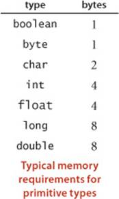
Analyzing memory usage is much easier than analyzing running time, primarily because not as many program statements are involved (just declarations) and because the analysis reduces complex objects to the primitive types, whose memory usage is well-defined and simple to understand: we can count up the number of variables and weight them by the number of bytes according to their type. For example, since the Java int data type is the set of integer values between —2,147,483,648 and 2,147,483,647, a grand total of 232 different values, typical Java implementations use 32 bits to represent int values. Similar considerations hold for other primitive types: typical Java implementations use 8-bit bytes, representing each char value with 2 bytes (16 bits), each int value with 4 bytes (32 bits), each double and each long value with 8 bytes (64 bits), and each boolean value with 1 byte (since computers typically access memory one byte at a time). Combined with knowledge of the amount of memory available, you can calculate limitations from these values. For example, if you have 1GB of memory on your computer (1 billion bytes or 230 bytes), you cannot fit more than about 256 million int values or 128 million double values in memory at any one time.
On the other hand, analyzing memory usage is subject to various differences in machine hardware and in Java implementations, so you should consider the specific examples that we give as indicative of how you might go about determining memory usage when warranted, not the final word for your computer. For example, many data structures involve representation of machine addresses, and the amount of memory needed for a machine address varies from machine to machine. For consistency, we assume that 8 bytes are needed to represent addresses, as is typical for 64-bit architectures that are now widely used, recognizing that many older machines use a 32-bit architecture that would involve just 4 bytes per machine address.
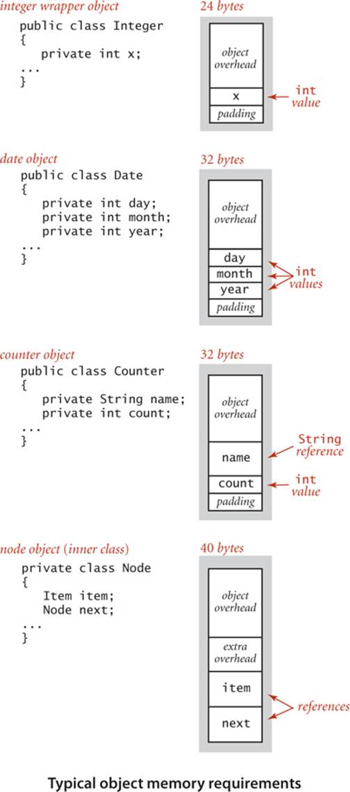
Objects
To determine the memory usage of an object, we add the amount of memory used by each instance variable to the overhead associated with each object, typically 16 bytes. The overhead includes a reference to the object’s class, garbage collection information, and synchronization information. Moreover, the memory usage is typically padded to be a multiple of 8 bytes (machine words, on a 64-bit machine). For example, an Integer object uses 24 bytes (16 bytes of overhead, 4 bytes for its int instance variable, and 4 bytes of padding). Similarly, a Date (page 91) object also uses 32 bytes: 16 bytes of overhead, 4 bytes for each of its three int instance variables, and 4 bytes of padding. A reference to an object typically is a memory address and thus uses 8 bytes of memory. For example, a Counter (page 89) object uses 32 bytes: 16 bytes of overhead, 8 bytes for its Stringinstance variable (a reference), 4 bytes for its int instance variable, and 4 bytes of padding. When we account for the memory for a reference, we account separately for the memory for the object itself, so this total does not count the memory for the String value.
Linked lists
A nested non-static (inner) class such as our Node class (page 142) requires an extra 8 bytes of overhead (for a reference to the enclosing instance). Thus, a Node object uses 40 bytes (16 bytes of object overhead, 8 bytes each for the references to the Item and Node objects, and 8 bytes for the extra overhead). Thus, since an Integer object uses 24 bytes, a stack with N integers built with a linked-list representation (ALGORITHM 1.2) uses 32 + 64N bytes, the usual 16 for object overhead for Stack, 8 for its reference instance variable, 4 for its int instance variable, 4 for padding, and 64 for each entry, 40 for a Node and 24 for an Integer.
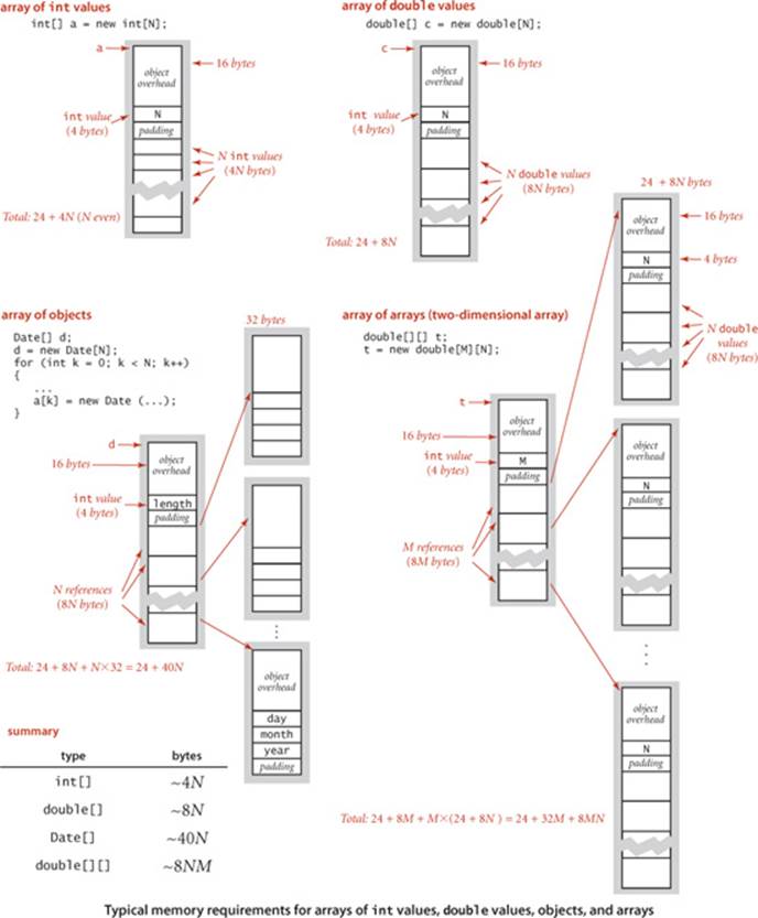
Arrays
Typical memory requirements for various types of arrays in Java are summarized in the diagrams on the facing page. Arrays in Java are implemented as objects, typically with extra overhead for the length. An array of primitive-type values typically requires 24 bytes of header information (16 bytes of object overhead, 4 bytes for the length, and 4 bytes of padding) plus the memory needed to store the values. For example, an array of N int values uses 24 + 4N bytes (rounded up to be a multiple of 8), and an array of N double values uses 24 + 8N bytes. An array of objects is an array of references to the objects, so we need to add the space for the references to the space required for the objects. For example, an array of N Date objects (page 91) uses 24 bytes (array overhead) plus 8N bytes (references) plus 32 bytes for each object, for a grand total of 24 + 40N bytes. A two-dimensional array is an array of arrays (each array is an object). For example, a two-dimensional M-by-N array of double values uses 24 bytes (overhead for the array of arrays) plus 8M bytes (references to the row arrays) plus M times 24 bytes (overhead from the row arrays) plus M times Ntimes 8 bytes (for the N double values in each of the M rows) for a grand total of 8NM + 32M + 24 ~ 8NM bytes. When array entries are objects, a similar accounting leads to a total of 8NM + 32M + 24 ~ 8NM bytes for the array of arrays filled with references to objects, plus the memory for the objects themselves.
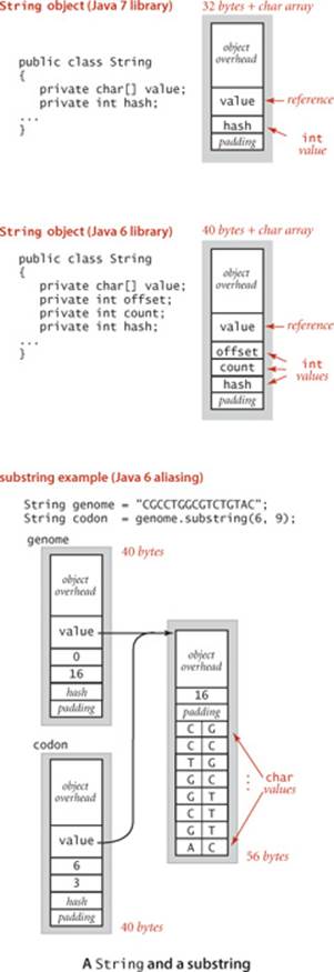
String objects (Java 7 and later)
The standard String representation (used in typical Java 7 implementitons) has two instance variables: a reference to a character array value[] that stores the sequence of characters and an int value hash (that stores a hash code that saves recomputation in certain circumstances that need not concern us now). Therefore, a String of length N typically uses 40 bytes for the String object (16 bytes for object overhead plus 8 bytes for the array reference plus 4 bytes for the int instance variables plus 4 bytes of padding) plus 24 + 2N bytes for the character array for a total of 56 + 2N bytes.
String objects (Java 6 and earlier)
An alternate String representation (used in typical Java 6 implementations) maintains two extra int instance variables (offset and count) and represents the sequence of characters value[offset] through value[offset + count - 1]. Now, a String of length N typically uses 40 bytes (for the String object) plus 24 + 2N bytes (for the character array) for a total of 64 + 2N bytes. This representation saves memory when extracting substrings because two String objects can share the same underlying character array.
Substring extraction
When using the Java 7 representation to implement the substring() method, we must create a new character array, so substring extraction takes linear time and linear space (in the length of the resulting substring). When using the Java 6 representation, we can implement the substring() method without having to make copies of the string’s characters: the character array containing the original string is aliased in the object for the substring; the offset and count fields identify the substring. Thus, a substring of an existing string takes just 40 bytes. In summary, extracting a substring takes either constant extra memory or linear extra memory depending on the underlying implementation. We will assume the Java 7 representation in this book.
THESE BASIC MECHANISMS ARE EFFECTIVE for estimating the memory usage of a great many programs, but there are numerous complicating factors that can make the task significantly more difficult. We have already noted the potential effect of aliasing. Moreover, memory consumption is a complicated dynamic process when function calls are involved because the system memory allocation mechanism plays a more important role, with more system dependencies. For example, when your program calls a method, the system allocates the memory needed for the method (for its local variables) from a special area of memory called the stack (a system pushdown stack), and when the method returns to the caller, the memory is returned to the stack. For this reason, creating arrays or other large objects in recursive programs is dangerous, since each recursive call implies significant memory usage. When you create an object with new, the system allocates the memory needed for the object from another special area of memory known as the heap (not the same as the binary heap data structure we consider in SECTION 2.4), and you must remember that every object lives until no references to it remain, at which point a system process known as garbage collection reclaims its memory for the heap. Such dynamics can make the task of precisely estimating memory usage of a program challenging.
Perspective
Good performance is important. An impossibly slow program is almost as useless as an incorrect one, so it is certainly worthwhile to pay attention to the cost at the outset, to have some idea of which kinds of problems you might feasibly address. In particular, it is always wise to have some idea of which code constitutes the inner loop of your programs.
Perhaps the most common mistake made in programming is to pay too much attention to performance characteristics. Your first priority is to make your code clear and correct. Modifying a program for the sole purpose of speeding it up is best left for experts. Indeed, doing so is often counterproductive, as it tends to create code that is complicated and difficult to understand. C. A. R. Hoare (the inventor of quicksort and a leading proponent of writing clear and correct code) once summarized this idea by saying that “premature optimization is the root of all evil,” to which Knuth added the qualifier “(or at least most of it) in programming.” Beyond that, improving the running time is not worthwhile if the available cost benefits are insignificant. For example, improving the running time of a program by a factor of 10 is inconsequential if the running time is only an instant. Even when a program takes a few minutes to run, the total time required to implement and debug an improved algorithm might be substantially more than the time required simply to run a slightly slower one—you may as well let the computer do the work. Worse, you might spend a considerable amount of time and effort implementing ideas that should in theory improve a program but do not do so in practice.
Perhaps the second most common mistake made in programming is to ignore performance characteristics. Faster algorithms are often more complicated than brute-force ones, so you might be tempted to accept a slower algorithm to avoid having to deal with more complicated code. However, you can sometimes reap huge savings with just a few lines of good code. Users of a surprising number of computer systems lose substantial time unknowingly waiting for brute-force quadratic algorithms to finish solving a problem, when linear or linearithmic algorithms are available that could solve the problem in a fraction of the time. When we are dealing with huge problem sizes, we often have no choice but to seek better algorithms.
We generally take as implicit the methodology described in this section to estimate memory usage and to develop an order-of-growth hypothesis of the running time from a tilde approximation resulting from a mathematical analysis within a cost model, and to check those hypotheses with experiments. Improving a program to make it more clear, efficient, and elegant should be your goal every time that you work on it. If you pay attention to the cost all the way through the development of a program, you will reap the benefits every time you use it.
Q&A
Q. Why not use StdRandom to generate random values instead of maintaining the file 1Mints.txt ?
A. It is easier to debug code in development and to reproduce experiments. StdRandom produces different values each time it is called, so running a program after fixing a bug may not test the fix! You could use StdRandom to address this problem, but a reference file such as 1Mints.txt makes it easier to add test cases while debugging. Also, different programmers can compare performance on different systems, without worrying about the input model. Once you have debugged a program and have a good idea of how it performs, it is certainly worthwhile to test it on random data. For example, DoublingTest and DoublingRatio take this approach.
Q. I ran DoublingRatio on my computer, but the results were not as consistent as in the book. Some of the ratios were not close to 8. Why?
A. That is why we discussed “caveats” on page 195. Most likely, your computer’s operating system decided to do something else during the experiment. One way to mitigate such problems is to invest more time in more experiments. For example, you could change DoublingTest to run the experiments 1,000 times for each N, giving a much more accurate estimate for the running time for each size (see EXERCISE 1.4.39).
Q. What, exactly, does “as N grows” mean in the definition of the tilde notation?
A. The formal definition of f(N) ~ g(N) is limN→∞ f(N)/g(N) = 1.
Q. I’ve seen other notations for describing order of growth. What’s the story?
A. The “big-Oh” notation is widely used: we say that f(N) is O(g(N)) if there exist constants c and N0 such that |f(N)|≤ c | g(N) for all N > N0. This notation is very useful in providing asymptotic upper bounds on the performance of algorithms, which is important in the theory of algorithms. But it is not useful for predicting performance or for comparing algorithms.
Q. Why not?
A. The primary reason is that it describes only an upper bound on the running time. Actual performance might be much better. The running time of an algorithm might be both O(N2) and ~ a N log N. As a result, it cannot be used to justify tests like our doubling ratio test (see PROPOSITION C on page 193).
Q. So why is the big-Oh notation so widely used?
A. It facilitates development of bounds on the order of growth, even for complicated algorithms for which more precise analysis might not be feasible. Moreover, it is compatible with the “big-Omega” and “big-Theta” notations that theoretical computer scientists use to classify algorithms by bounding their worst-case performance. We say that f(N) is Ω(g(N)) if there exist constants c and N0 such that |f(N)| ≥ c | g(N) for N > N0; and if f(N) is O(g(N)) and Ω(g(N)), we say that f(N) is Θ(g(N)). The “big-Omega” notation is typically used to describe a lower bound on the worst case, and the “big-Theta” notation is typically used to describe the performance of algorithms that are optimal in the sense that no algorithm can have better asymptotic worst-case order of growth. Optimal algorithms are certainly worth considering in practical applications, but there are many other considerations, as you will see.
Q. Aren’t upper bounds on asymptotic performance important?
A. Yes, but we prefer to discuss precise results in terms of frequency of statement exceution with respect to cost models, because they provide more information about algorithm performance and because deriving such results is feasible for the algorithms that we discuss. For example, we say “ThreeSum uses ~N3/2 array accesses” and “the number of times cnt++ is executed in ThreeSum is ~N3/6 in the worst case,” which is a bit more verbose but much more informative than the statement “the running time of ThreeSum is O(N3).”
Q. When the order of growth of the running time of an algorithm is N log N, the doubling test will lead to the hypothesis that the running time is ~a N for a constant a. Isn’t that a problem?
A. We have to be careful not to try to infer that the experimental data implies a particular mathematical model, but when we are just predicting performance, this is not really a problem. For example, when N is between 16,000 and 32,000, the plots of 14N and N lg N are very close to one another. The data fits both curves. As N increases, the curves become closer together. It actually requires some care to experimentally check the hypothesis that an algorithm’s running time is linearithmic but not linear.
Q. Does int[] a = new int[N] count as N array accesses (to initialize entries to 0)?
A. Most likely yes, so we make that assumption in this book, though a sophisticated compiler implementation might try to avoid this cost for huge sparse arrays.
Exercises
1.4.1 Show that the number of different triples that can be chosen from N items is precisely N(N–1)(N–2)/6. Hint: Use mathematical induction.
1.4.2 Modify ThreeSum to work properly even when the int values are so large that adding two of them might cause overflow.
1.4.3 Modify DoublingTest to use StdDraw to produce plots like the standard and log-log plots in the text, rescaling as necessary so that the plot always fills a substantial portion of the window.
1.4.4 Develop a table like the one on page 181 for TwoSum.
1.4.5 Give tilde approximations for the following quantities:
a. N + 1
b. 1 + 1/N
c. (1 + 1/N)(1 + 2/N)
d. 2N3− 15 N2 + N
e. lg(2N)/lg N
f. lg(N2 + 1) / lg N
g. N100 / 2N
1.4.6 Give the order of growth (as a function of N) of the running times of each of the following code fragments:
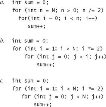
1.4.7 Analyze ThreeSum under a cost model that counts arithmetic operations (and comparisons) involving the input numbers.
1.4.8 Write a program to determine the number pairs of values in an input file that are equal. If your first try is quadratic, think again and use Arrays.sort() to develop a linearithmic solution.
1.4.9 Give a formula to predict the running time of a program for a problem of size N when doubling experiments have shown that the doubling factor is 2b and the running time for problems of size N0 is T.
1.4.10 Modify binary search so that it always returns the element with the smallest index that matches the search element (and still guarantees logarithmic running time).
1.4.11 Add an instance method howMany() to StaticSETofInts (page 99) that finds the number of occurrences of a given key in time proportional to log N in the worst case.
1.4.12 Write a program that, given two sorted arrays of N int values, prints all elements that appear in both arrays, in sorted order. The running time of your program should be proportional to N in the worst case.
1.4.13 Using the assumptions developed in the text, give the amount of memory needed to represent an object of each of the following types:
a. Accumulator
b. Transaction
c. FixedCapacityStackOfStrings with capacity C and N entries
d. Point2D
e. Interval1D
f. Interval2D
g. Double
Creative Problems
1.4.14 4-sum. Develop an algorithm for the 4-sum problem.
1.4.15 Faster 3-sum. As a warmup, develop an implementation TwoSumFaster that uses a linear algorithm to count the pairs that sum to zero after the array is sorted (instead of the binary-search-based linearithmic algorithm). Then apply a similar idea to develop a quadratic algorithm for the 3-sum problem.
1.4.16 Closest pair (in one dimension). Write a program that, given an array a[] of N double values, finds a closest pair: two values whose difference is no greater than the the difference of any other pair (in absolute value). The running time of your program should be linearithmic in the worst case.
1.4.17 Farthest pair (in one dimension). Write a program that, given an array a[] of N double values, finds a farthest pair: two values whose difference is no smaller than the the difference of any other pair (in absolute value). The running time of your program should be linear in the worst case.
1.4.18 Local minimum of an array. Write a program that, given an array a[] of N distinct integers, finds a local minimum: entry a[i] that is strictly less than its neighbors. Each internal entry (other than a[0] and a[N-1]) has 2 neighbors. Your program should use ~2lg N compares in the worst case.
1.4.19 Local minimum of a matrix. Given an N-by-N array a[] of N2 distinct integers, design an algorithm that finds a local minimum: an entry a[i][j] that is strictly less than its neighbors. Internal entries have 4 neighbors; entries on an edge have 3 neighbors; entries on a corner have 2 neighbors. The running time of your program should be proportional to N in the worst case, which means that you cannot afford to examine all N2 entries.
1.4.20 Bitonic search. An array is bitonic if it is comprised of an increasing sequence of integers followed immediately by a decreasing sequence of integers. Write a program that, given a bitonic array of N distinct int values, determines whether a given integer is in the array. Your program should use ~3lg N compares in the worst case. Extra credit: use only ~2 lg N compares in the worst case.
1.4.21 Binary search on distinct values. Develop an implementation of binary search for StaticSETofInts (see page 99) where the running time of contains() is guaranteed to be ~ lg R, where R is the number of different integers in the array given as argument to the constructor.
1.4.22 Binary search with only addition and subtraction. [Mihai Patrascu] Write a program that, given an array of N distinct int values in ascending order, determines whether a given integer is in the array. You may use only additions and subtractions and a constant amount of extra memory. The running time of your program should be proportional to log N in the worst case.
1.4.23 Binary search for a fraction. Devise a method that uses a logarithmic number of compares of the form Is the number less than x? to find a rational number p/q such that 0 < p < q < N. Hint: Two different fractions with denominators less than N must differ by at least /N2.
1.4.24 Throwing eggs from a building. Suppose that you have an N-story building and plenty of eggs. Suppose also that an egg is broken if it is thrown off floor F or higher, and hurt otherwise. First, devise a strategy to determine the value of F such that the number of broken eggs is ~lg Nwhen using ~lg N throws, then find a way to reduce the cost to ~2lg F.
1.4.25 Throwing two eggs from a building. Consider the previous question, but now suppose you only have two eggs, and your cost model is the number of throws. Devise a strategy to determine F such that the number of throws is at most 2√N, then find a way to reduce the cost to ~c√F for some constant c. This is analogous to a situation where search hits (egg intact) are much cheaper than misses (egg broken).
1.4.26 3-collinearity. Suppose that you have an algorithm that takes as input N distinct points in the plane and can return the number of triples that fall on the same line. Show that you can use this algorithm to solve the 3-sum problem. Strong hint: Use algebra to show that (a, a3), (b, b3), and (c, c3) are collinear if and only if a + b + c = 0.
1.4.27 Queue with two stacks. Implement a queue with two stacks so that each queue operation takes a constant amortized number of stack operations. Hint: If you push elements onto a stack and then pop them all, they appear in reverse order. If you repeat this process, they’re now back in order.
1.4.28 Stack with a queue. Implement a stack with a single queue so that each stack operations takes a linear number of queue operations. Hint: To delete an item, get all of the elements on the queue one at a time, and put them at the end, except for the last one which you should delete and return. (This solution is admittedly very inefficient.)
1.4.29 Steque with two stacks. Implement a steque with two stacks so that each steque operation (see EXERCISE 1.3.32) takes a constant amortized number of stack operations.
1.4.30 Deque with a stack and a steque. Implement a deque with a stack and a steque (see EXERCISE 1.3.32) so that each deque operation takes a constant amortized number of stack and steque operations.
1.4.31 Deque with three stacks. Implement a deque with three stacks so that each deque operation takes a constant amortized number of stack operations.
1.4.32 Amortized analysis. Prove that, starting from an empty stack, the number of array accesses used by any sequence of M operations in the resizing array implementation of Stack is proportional to M.
1.4.33 Memory requirements on a 32-bit machine. Give the memory requirements for Integer, Date, Counter, int[], double[], double[][], String, Node, and Stack (linked-list representation) for a 32-bit machine. Assume that references are 4 bytes, object overhead is 8 bytes, and padding is to a multiple of 4 bytes.
1.4.34 Hot or cold. Your goal is to guess a secret integer between 1 and N. You repeatedly guess integers between 1 and N. After each guess you learn if your guess equals the secret integer (and the game stops). Otherwise, you learn if the guess is hotter (closer to) or colder (farther from) the secret number than your previous guess. Design an algorithm that finds the secret number in at most ~2 lg N guesses. Then design an algorithm that finds the secret number in at most ~ 1 lg N guesses.
1.4.35 Time costs for pushdown stacks. Justify the entries in the table below, which shows typical time costs for various pushdown stack implementations, using a cost model that counts both data references (references to data pushed onto the stack, either an array reference or a reference to an object’s instance variable) and objects created. Assume that the Integer objects are not cached (so they must be created for each push).
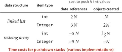
1.4.36 Space usage for pushdown stacks. Justify the entries in the table below, which shows typical space usage for various pushdown stack implementations. Use a static nested class for linked-list nodes to avoid the non-static nested class overhead. Assume that the Integer objects are not cached (so they must be created for each push).
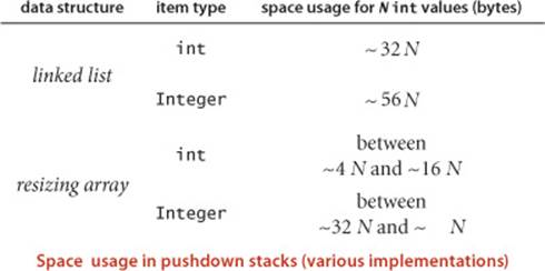
Experiments
1.4.37 Autoboxing performance penalty. Run experiments to determine the performance penalty on your machine for using autoboxing and auto-unboxing. Develop an implementation FixedCapacityStackOfInts and use a client such as DoublingRatio to compare its performance with the genericFixedCapacityStack<Integer>, for a large number of push() and pop() operations.
1.4.38 Naive 3-sum implementation. Run experiments to evaluate the following implementation of the inner loop of ThreeSum:
for (int i = 0; i < N; i++)
for (int j = 0; j < N; j++)
for (int k = 0; k < N; k++)
if (i < j && j < k)
if (a[i] + a[j] + a[k] == 0)
cnt++;
Do so by developing a version of DoublingTest that computes the ratio of the running times of this program and ThreeSum.
1.4.39 Improved accuracy for doubling test. Modify DoublingRatio to take a second command-line argument that specifies the number of calls to make to timeTrial() for each value of N. Run your program for 10, 100, and 1,000 trials and comment on the precision of the results.
1.4.40 3-sum for random values. Formulate and validate a hypothesis describing the number of triples of N random int values that sum to 0. If you are skilled in mathematical analysis, develop an appropriate mathematical model for this problem, where the values are uniformly distributed between –M and M, where M is not small.
1.4.41 Running times. Estimate the amount of time it would take to run TwoSumFast, TwoSum, ThreeSumFast and ThreeSum on your computer to solve the problems for a file of 1 million numbers. Use DoublingRatio to do so.
1.4.42 Problem sizes. Estimate the size of the largest value of P for which you can run TwoSumFast, TwoSum, ThreeSumFast, and ThreeSum on your computer to solve the problems for a file of 2P thousand numbers. Use DoublingRatio to do so.
1.4.43 Resizing arrays versus linked lists. Run experiments to validate the hypothesis that resizing arrays are faster than linked lists for stacks (see EXERCISE 1.4.35 and EXERCISE 1.4.36). Do so by developing a version of DoublingRatio that computes the ratio of the running times of the two programs.
1.4.44 Birthday problem. Write a program that takes an integer N from the command line and uses StdRandom.uniform() to generate a random sequence of integers between 0 and N − 1. Run experiments to validate the hypothesis that the number of integers generated before the first repeated value is found is ![]() .
.
1.4.45 Coupon collector problem. Generating random integers as in the previous exercise, run experiments to validate the hypothesis that the number of integers generated before all possible values are generated is ~N HN.
All materials on the site are licensed Creative Commons Attribution-Sharealike 3.0 Unported CC BY-SA 3.0 & GNU Free Documentation License (GFDL)
If you are the copyright holder of any material contained on our site and intend to remove it, please contact our site administrator for approval.
© 2016-2026 All site design rights belong to S.Y.A.