Algorithms (2014)
Two. Sorting
2.2 Mergesort
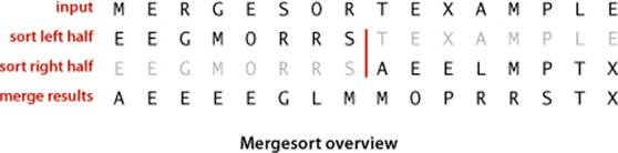
THE ALGORITHMS that we consider in this section are based on a simple operation known as merging: combining two ordered arrays to make one larger ordered array. This operation immediately leads to a simple recursive sort method known as mergesort: to sort an array, divide it into two halves, sort the two halves (recursively), and then merge the results. As you will see, one of mergesort’s most attractive properties is that it guarantees to sort any array of N items in time proportional to N log N. Its prime disadvantage is that it uses extra space proportional to N.
Abstract in-place merge
The straightforward approach to implementing merging is to design a method that merges two disjoint ordered arrays of Comparable objects into a third array. This strategy is easy to implement: create an output array of the requisite size and then choose successively the smallest remaining item from the two input arrays to be the next item added to the output array.
However, when we mergesort a large array, we are doing a huge number of merges, so the cost of creating a new array to hold the output every time that we do a merge is problematic. It would be much more desirable to have an in-place method so that we could sort the first half of the array in place, then sort the second half of the array in place, then do the merge of the two halves by moving the items around within the array, without using a significant amount of other extra space. It is worthwhile to pause momentarily to consider how you might do that. At first blush, this problem seems to be one that must be simple to solve, but solutions that are known are quite complicated, especially by comparison to alternatives that use extra space.
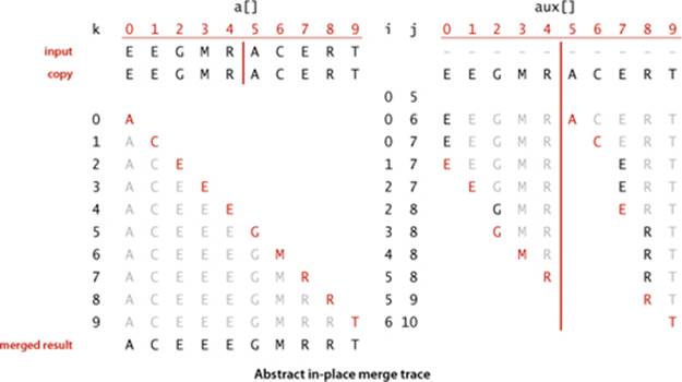
Still, the abstraction of an in-place merge is useful. Accordingly, we use the method signature merge(a, lo, mid, hi) to specify a merge method that puts the result of merging the subarrays a[lo..mid] with a[mid+1..hi] into a single ordered array, leaving the result in a[lo..hi]. The code on the next page implements this merge method in just a few lines by copying everything to an auxiliary array and then merging back to the original. Another approach is described in EXERCISE 2.2.9.
Abstract in-place merge
public static void merge(Comparable[] a, int lo, int mid, int hi)
{ // Merge a[lo..mid] with a[mid+1..hi].
int i = lo, j = mid+1;
for (int k = lo; k <= hi; k++) // Copy a[lo..hi] to aux[lo..hi].
aux[k] = a[k];
for (int k = lo; k <= hi; k++) // Merge back to a[lo..hi].
if (i > mid) a[k] = aux[j++];
else if (j > hi ) a[k] = aux[i++];
else if (less(aux[j], aux[i])) a[k] = aux[j++];
else a[k] = aux[i++];
}
This method merges by first copying into the auxiliary array aux[] then merging back to a[]. In the merge (the second for loop), there are four conditions: left half exhausted (take from the right), right half exhausted (take from the left), current key on right less than current key on left (take from the right), and current key on right greater than or equal to current key on left (take from the left).
Top-down mergesort
ALGORITHM 2.4 is a recursive mergesort implementation based on this abstract in-place merge. It is one of the best-known examples of the utility of the divide-and-conquer paradigm for efficient algorithm design. This recursive code is the basis for an inductive proof that the algorithm sorts the array: if it sorts the two subarrays, it sorts the whole array, by merging together the subarrays.
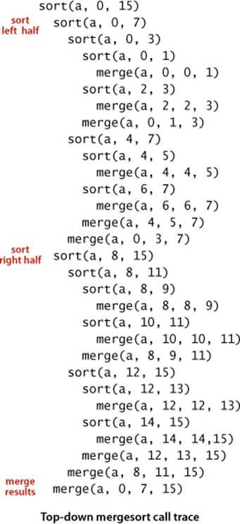
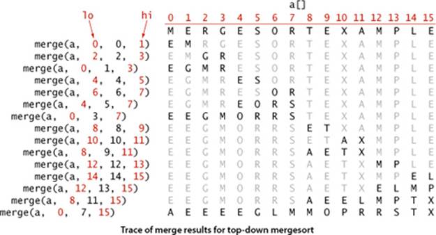
To understand mergesort, it is worthwhile to consider carefully the dynamics of the method calls, shown in the trace at right. To sort a[0..15], the sort() method calls itself to sort a[0..7] then calls itself to sort a[0..3] and a[0..1] before finally doing the first merge of a[0] with a[1] after calling itself to sort a[0] and then a[1] (for brevity, we omit the calls for the base-case 1-entry sorts in the trace). Then the next merge is a[2] with a[3] and then a[0..1] with a[2..3] and so forth. From this trace, we see that the sort code simply provides an organized way to sequence the calls to the merge()method. This insight will be useful later in this section.
The recursive code also provides us with the basis for analyzing mergesort’s running time. Because mergesort is a prototype of the divide-and-conquer algorithm design paradigm, we will consider this analysis in detail.
Proposition F. Top-down mergesort uses between ½ N lg N and N lgN compares to sort any array of length N.
Proof: Let C(N) be the number of compares needed to sort an array of length N. We have C(0) = C(1) = 0 and for N > 0 we can write a recurrence relationship that directly mirrors the recursive sort() method to establish an upper bound:
C(N) ≤ C(![]() N/2
N/2![]() ) + C(
) + C(![]() N/2
N/2![]() ) + N.
) + N.
The first term on the right is the number of compares to sort the left half of the array, the second term is the number of compares to sort the right half, and the third term is the number of compares for the merge. The lower bound
C(N) ≥ C(![]() N/2
N/2![]() )+ C(
)+ C(![]() N/2
N/2![]() ) +
) + ![]() N/2
N/2![]()
follows because the number of compares for the merge is at least ![]() N/2
N/2![]() .
.
We derive an exact solution to the recurrence when equality holds and N is a power of 2 (say N = 2n). First, since ![]() N/2
N/2![]() =
= ![]() N/2
N/2![]() = 2n−1, we have
= 2n−1, we have
C(2n) = 2C(2n−1) + 2n.
Dividing both sides by 2n gives
C(2n)/2n = C(2n−1)/2n−1 + 1.
Applying the same equation to the first term on the right, we have
C(2n)/2n = C(2n−2)/2n−2 + 1 + 1.
Repeating the previous step n − 1 additional times gives
C(2n)/2n = C(20)/20 + n.
which, after multiplying both sides by 2n, leaves us with the solution
C(N) = C(2n) = n 2n = N lgN.
Exact solutions for general N are more complicated, but it is not difficult to apply the same argument to the inequalities describing the bounds on the number of compares to prove the stated result for all values of N. This proof is valid no matter what the input values are and no matter in what order they appear.
Algorithm 2.4 Top-down mergesort
public class Merge
{
private static Comparable[] aux; // auxiliary array for merges
public static void sort(Comparable[] a)
{
aux = new Comparable[a.length]; // Allocate space just once.
sort(a, 0, a.length - 1);
}
private static void sort(Comparable[] a, int lo, int hi)
{ // Sort a[lo..hi].
if (hi <= lo) return;
int mid = lo + (hi - lo)/2;
sort(a, lo, mid); // Sort left half.
sort(a, mid+1, hi); // Sort right half.
merge(a, lo, mid, hi); // Merge results (code on page 271).
}
}
To sort a subarray a[lo..hi] we divide it into two parts: a[lo..mid] and a[mid+1..hi], sort them independently (via recursive calls), and merge the resulting ordered subarrays to produce the result.
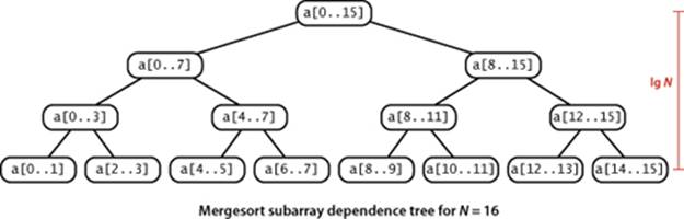
Another way to understand PROPOSITION F is to examine the tree drawn below, where each node depicts a subarray for which sort() does a merge(). The tree has precisely n levels. For k from 0 to n − 1, the kth level from the top depicts 2k subarrays, each of length 2n−k, each of which thus requires at most 2n−k compares for the merge. Thus we have 2k · 2n−k = 2n total cost for each of the n levels, for a total of n 2n = N lgN.
Proposition G. Top-down mergesort uses at most 6N lgN array accesses to sort an array of length N.
Proof: Each merge uses at most 6N array accesses (2N for the copy, 2N for the move back, and at most 2N for compares). The result follows from the same argument as for PROPOSITION F.
PROPOSITIONS F and G tell us that we can expect the time required by mergesort to be proportional to N log N. That fact brings us to a different level from the elementary methods in SECTION 2.1 because it tells us that we can sort huge arrays using just a logarithmic factor more time than it takes to examine every entry. You can sort millions of items (or more) with mergesort, but not with insertion sort or selection sort. The primary drawback of mergesort is that it requires extra space proportional to N, for the auxiliary array for merging. If space is at a premium, we need to consider another method. On the other hand, we can cut the running time of mergesort substantially with some carefully considered modifications to the implementation.
Use insertion sort for small subarrays
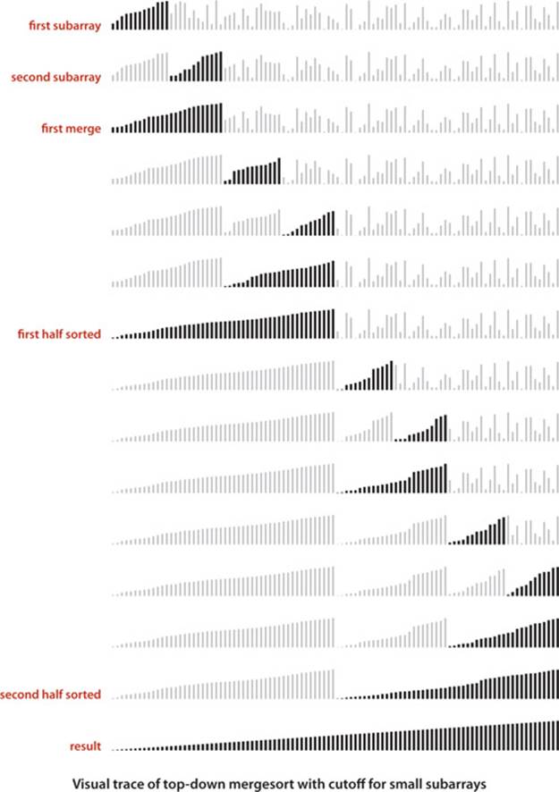
We can improve most recursive algorithms by handling small cases differently, because the recursion guarantees that the method will be used often for small cases, so improvements in handling them lead to improvements in the whole algorithm. In the case of sorting, we know that insertion sort (or selection sort) is simple and therefore likely to be faster than mergesort for tiny subarrays. As usual, a visual trace provides insight into the operation of mergesort. The visual trace on the next page shows the operation of a mergesort implementation with a cutoff for small subarrays. Switching to insertion sort for small subarrays (length 15 or less, say) will improve the running time of a typical mergesort implementation by 10 to 15 percent (see EXERCISE 2.2.23).
Test whether the array is already in order
We can reduce the running time to be linear for arrays that are already in order by adding a test to skip the call to merge() if a[mid] is less than or equal to a[mid+1]. With this change, we still do all the recursive calls, but the running time for any sorted subarray is linear (see EXERCISE 2.2.8).
Eliminate the copy to the auxiliary array
It is possible to eliminate the time (but not the space) taken to copy to the auxiliary array used for merging. To do so, we use two invocations of the sort method: one takes its input from the given array and puts the sorted output in the auxiliary array; the other takes its input from the auxiliary array and puts the sorted output in the given array. With this approach, in a bit of recursive trickery, we can arrange the recursive calls such that the computation switches the roles of the input array and the auxiliary array at each level (see EXERCISE 2.2.11).
It is appropriate to repeat here a point raised in CHAPTER 1 that is easily forgotten and needs reemphasis. Locally, we treat each algorithm in this book as if it were critical in some application. Globally, we try to reach general conclusions about which approach to recommend. Our discussion of such improvements is not necessarily a recommendation to always implement them, rather a warning not to draw absolute conclusions about performance from initial implementations. When addressing a new problem, your best bet is to use the simplest implementation with which you are comfortable and then refine it if it becomes a bottleneck. Addressing improvements that decrease running time just by a constant factor may not otherwise be worthwhile. You need to test the effectiveness of specific improvements by running experiments, as we indicate in exercises throughout.
In the case of mergesort, the three improvements just listed are simple to implement and are of interest when mergesort is the method of choice—for example, in situations discussed at the end of this chapter.
Bottom-up mergesort
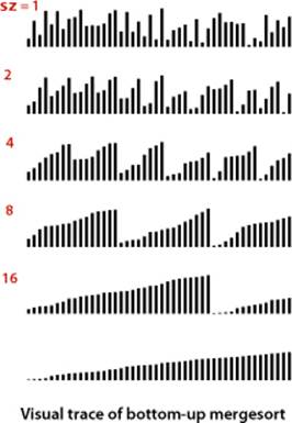
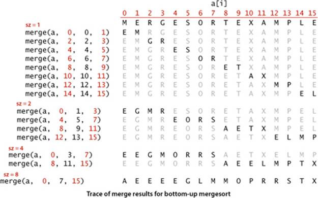
The recursive implementation of mergesort is prototypical of the divide-and-conquer algorithm design paradigm, where we solve a large problem by dividing it into pieces, solving the subproblems, then using the solutions for the pieces to solve the whole problem. Even though we are thinking in terms of merging together two large subarrays, the fact is that most merges are merging together tiny subarrays. Another way to implement mergesort is to organize the merges so that we do all the merges of tiny subarrays on one pass, then do a second pass to merge those subarrays in pairs, and so forth, continuing until we do a merge that encompasses the whole array. This method requires even less code than the standard recursive implementation. We start by doing a pass of 1-by-1 merges (considering individual items as subarrays of size 1), then a pass of 2-by-2 merges (merge subarrays of size 2 to make subarrays of size 4), then 4-by-4 merges, and so forth. The second subarray may be smaller than the first in the last merge on each pass (which is no problem for merge()), but otherwise all merges involve subarrays of equal size, doubling the sorted subarray size for the next pass.
Bottom-up mergesort
public class MergeBU
{
private static Comparable[] aux; // auxiliary array for merges
// See page 271 for merge() code.
public static void sort(Comparable[] a)
{ // Do lg N passes of pairwise merges.
int N = a.length;
aux = new Comparable[N];
for (int sz = 1; sz < N; sz = sz+sz) // sz: subarray size
for (int lo = 0; lo < N-sz; lo += sz+sz) // lo: subarray index
merge(a, lo, lo+sz-1, Math.min(lo+sz+sz-1, N-1));
}
}
Bottom-up mergesort consists of a sequence of passes over the whole array, doing sz-by-sz merges, starting with sz equal to 1 and doubling sz on each pass. The final subarray is of size sz only when the array size is an even multiple of sz (otherwise it is less than sz).
Proposition H. Bottom-up mergesort uses between ½ N lg N and N lg N compares and at most 6N lg N array accesses to sort an array of length N.
Proof: The number of passes through the array is precisely ![]() lg N
lg N![]() (that is precisely the value of n such that 2n-1 ≤ N < 2n+1). For each pass, the number of array accesses is exactly 6N and the number of compares is at most N and no less than N/2.
(that is precisely the value of n such that 2n-1 ≤ N < 2n+1). For each pass, the number of array accesses is exactly 6N and the number of compares is at most N and no less than N/2.
WHEN THE ARRAY LENGTH IS A POWER OF 2, top-down and bottom-up mergesort perform precisely the same compares and array accesses, just in a different order. When the array length is not a power of 2, the sequence of compares and array accesses for the two algorithms will be different (seeEXERCISE 2.2.5).
A version of bottom-up mergesort is the method of choice for sorting data organized in a linked list. Consider the list to be sorted sublists of size 1, then pass through to make sorted sublists of size 2 linked together, then size 4, and so forth. This method rearranges the links to sort the list in place (without creating any new list nodes).
Both the top-down and bottom-up approaches to implementing a divide-and-conquer algorithm are intuitive. The lesson that you can take from mergesort is this: Whenever you encounter an algorithm based on one of these approaches, it is worth considering the other. Do you want to solve the problem by breaking it up into smaller problems (and solving them recursively) as in Merge.sort() or by building small solutions into larger ones as in MergeBU.sort()?
The complexity of sorting
One important reason to know about mergesort is that we use it as the basis for proving a fundamental result in the field of computational complexity that helps us understand the intrinsic difficulty of sorting. In general, computational complexity plays an important role in the design of algorithms, and this result in particular is directly relevant to the design of sorting algorithms, so we next consider it in detail.
The first step in a study of complexity is to establish a model of computation. Generally, researchers strive to understand the simplest model relevant to a problem. For sorting, we study the class of compare-based algorithms that make their decisions about items only on the basis of comparing keys. A compare-based algorithm can do an arbitrary amount of computation between compares, but cannot get any information about a key except by comparing it with another one. Because of our restriction to the Comparable API, all of the algorithms in this chapter are in this class (note that we are ignoring the cost of array accesses), as are many algorithms that we might imagine. In CHAPTER 5, we consider algorithms that are not restricted to Comparable items.
Proposition I. No compare-based sorting algorithm can guarantee to sort N items with fewer than lg(N!) ~ N lg N compares.
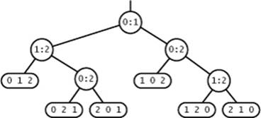
Proof: First, we assume that the keys are all distinct, since any algorithm must be able to sort such inputs. Now, we use a binary tree to describe the sequence of compares. Each node in the tree is either a leaf ![]() that indicates that the sort is complete and has discovered that the original inputs were in the order a[i0], a[i1], ...a[iN-1], or an internal node
that indicates that the sort is complete and has discovered that the original inputs were in the order a[i0], a[i1], ...a[iN-1], or an internal node ![]() that corresponds to a compare operation between a[i] and a[j], with a left subtree corresponding to the sequence of compares in the case that a[i] is less than a[j], and a right subtree corresponding to what happens if a[i] is greater than a[j]. Each path from the root to a leaf corresponds to the sequence of compares that the algorithm uses to establish the ordering given in the leaf. For example, here is a compare tree for N = 3:
that corresponds to a compare operation between a[i] and a[j], with a left subtree corresponding to the sequence of compares in the case that a[i] is less than a[j], and a right subtree corresponding to what happens if a[i] is greater than a[j]. Each path from the root to a leaf corresponds to the sequence of compares that the algorithm uses to establish the ordering given in the leaf. For example, here is a compare tree for N = 3:
We never explicitly construct such a tree—it is a mathematical device for describing the compares used by any algorithm.
The first key observation in the proof is that the tree must have at least N! leaves because there are N! different permutations of N distinct keys. If there are fewer than N! leaves, then some permutation is missing from the leaves, and the algorithm would fail for that permutation.
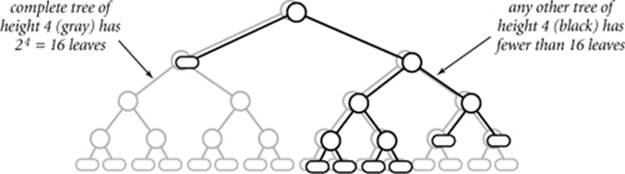
The number of internal nodes on a path from the root to a leaf in the tree is the number of compares used by the algorithm for some input. We are interested in the length of the longest such path in the tree (known as the tree height) since it measures the worst-case number of compares used by the algorithm. Now, it is a basic combinatorial property of binary trees that a tree of height h has no more than 2h leaves—the tree of height h with the maximum number of leaves is perfectly balanced, or complete. An example for h = 4 is diagrammed on the next page.
Combining the previous two paragraphs, we have shown that any compare-based sorting algorithm corresponds to a compare tree of height h with
N! ≤ number of leaves ≤ 2h
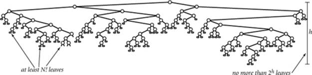
The value of h is precisely the worst-case number of compares, so we can take the logarithm (base 2) of both sides of this equation and conclude that the number of compares used by any algorithm must be at least lg (N!). The approximation lg N! ~ N lg N follows immediately from Stirling’s approximation to the factorial function (see page 185).
This result serves as a guide for us to know, when designing a sorting algorithm, how well we can expect to do. For example, without such a result, one might set out to try to design a compare-based sorting algorithm that uses half as many compares as does mergesort, in the worst case. The lower bound in PROPOSITION I says that such an effort is futile—no such algorithm exists. It is an extremely strong statement that applies to any conceivable compare-based algorithm.
PROPOSITION H asserts that the number of compares used by mergesort in the worst case is ~ N lg N. This result is an upper bound on the difficulty of the sorting problem in the sense that a better algorithm would have to guarantee to use a smaller number of compares. PROPOSITION I asserts that no sorting algorithm can guarantee to use fewer than ~ N lg N compares. It is a lower bound on the difficulty of the sorting problem in the sense that even the best possible algorithm must use at least that many compares in the worst case. Together, they imply:
Proposition J. Mergesort is an asymptotically optimal compare-based sorting algorithm.
Proof: Precisely, we mean by this statement that both the number of compares used by mergesort in the worst case and the minimum number of compares that any compare-based sorting algorithm can guarantee are ~N lg N. PROPOSITIONS H and I establish these facts.
It is important to note that, like the model of computation, we need to precisely define what we mean by an optimal algorithm. For example, we might tighten the definition of optimality and insist that an optimal algorithm for sorting is one that uses precisely lg (N!) compares. We do not do so because we could not notice the difference between such an algorithm and (for example) mergesort for large N. Or, we might broaden the definition of optimality to include any sorting algorithm whose worst-case number of compares is within a constant factor of N lg N. We do not do so because we might very well notice the difference between such an algorithm and mergesort for large N.
COMPUTATIONAL COMPLEXITY MAY SEEM RATHER ABSTRACT, but fundamental research on the intrinsic difficulty of solving computational problems hardly needs justification. Moreover, when it does apply, it is emphatically the case that computational complexity affects the development of good software. First, good upper bounds allow software engineers to provide performance guarantees; there are many documented instances where poor performance has been traced to someone using a quadratic sort instead of a linearithmic one. Second, good lower bounds spare us the effort of searching for performance improvements that are not attainable.
But the optimality of mergesort is not the end of the story and should not be misused to indicate that we need not consider other methods for practical applications. That is not the case because the theory in this section has a number of limitations. For example:
• Mergesort is not optimal with respect to space usage.
• The worst case may not be likely in practice.
• Operations other than compares (such as array accesses) may be important.
• One can sort certain data without using any compares.
Thus, we shall be considering several other sorting methods in this book.
Q&A
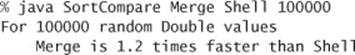
Q. Is mergesort faster than shellsort?
A. In practice, their running times are within a small constant factor of one another (when shellsort is using a well-tested increment sequence like the one in ALGORITHM 2.3), so comparative performance depends on the implementations.
In theory, no one has been able to prove that shellsort is linearithmic for random data, so there remains the possibility that the asymptotic growth of the average-case performance of shellsort is higher. Such a gap has been proven for worst-case performance, but it is not relevant in practice.
Q. Why not make the aux[] array local to merge()?
A. To avoid the overhead of creating an array for every merge, even the tiny ones. This cost would dominate the running time of mergesort (see EXERCISE 2.2.26). A more proper solution (which we avoid in the text to reduce clutter in the code) is to make aux[] local to sort() and pass it as an argument to merge() (see EXERCISE 2.2.9).
Q. How does mergesort fare when there are duplicate values in the array?
A. If all the items have the same value, the running time is linear (with the extra test to skip the merge when the array is sorted), but if there is more than one duplicate value, this performance gain is not necessarily realized. For example, suppose that the input array consists of N items with one value in odd positions and N items with another value in even positions. The running time is linearithmic for such an array (it satisfies the same recurrence as for items with distinct values), not linear.
Exercises
2.2.1 Give a trace, in the style of the trace given at the beginning of this section, showing how the keys A E Q S U Y E I N O S T are merged with the abstract in-place merge() method.
2.2.2 Give traces, in the style of the trace given with ALGORITHM 2.4, showing how the keys E A S Y Q U E S T I O N are sorted with top-down mergesort.
2.2.3 Answer EXERCISE 2.2.2 for bottom-up mergesort.
2.2.4 Does the abstract in-place merge produce proper output if and only if the two input subarrays are in sorted order? Prove your answer, or provide a counterexample.
2.2.5 Give the sequence of subarray sizes in the merges performed by both the top-down and the bottom-up mergesort algorithms, for N = 39.
2.2.6 Write a program to compute the exact value of the number of array accesses used by top-down mergesort and by bottom-up mergesort. Use your program to plot the values for N from 1 to 512, and to compare the exact values with the upper bound 6N lg N.
2.2.7 Show that the number of compares used by mergesort is monotonically increasing (C(N+1) > C(N) for all N > 0).
2.2.8 Suppose that ALGORITHM 2.4 is modified to skip the call on merge() whenever a[mid] <= a[mid+1]. Prove that the number of compares used to mergesort a sorted array is linear.
2.2.9 Use of a static array like aux[] is inadvisable in library software because multiple clients might use the class concurrently. Give an implementation of Merge that does not use a static array. Do not make aux[] local to merge() (see the Q&A for this section). Hint: Pass the auxiliary array as an argument to the recursive sort().
Creative Problems
2.2.10 Faster merge. Implement a version of merge() that copies the second half of a[] to aux[] in decreasing order and then does the merge back to a[]. This change allows you to remove the code to test that each of the halves has been exhausted from the inner loop. Note: The resulting sort is not stable (see page 341).
2.2.11 Improvements. Implement the three improvements to mergesort that are described in the text on page 275: Add a cutoff for small subarrays, test whether the array is already in order, and avoid the copy by switching arguments in the recursive code.
2.2.12 Sublinear extra space. Develop a merge implementation that reduces the extra space requirement to max(M, N/M), based on the following idea: Divide the array into N/M blocks of size M (for simplicity in this description, assume that N is a multiple of M). Then, (i) considering the blocks as items with their first key as the sort key, sort them using selection sort; and (ii) run through the array merging the first block with the second, then the second block with the third, and so forth.
2.2.13 Lower bound for average case. Prove that the expected number of compares used by any compare-based sorting algorithm must be at least ~N lg N (assuming that all possible orderings of the input are equally likely). Hint: The expected number of compares is at least the external path length of the compare tree (the sum of the lengths of the paths from the root to all leaves), which is minimized when it is balanced.
2.2.14 Merging sorted queues. Develop a static method that takes two queues of sorted items as arguments and returns a queue that results from merging the queues into sorted order.
2.2.15 Bottom-up queue mergesort. Develop a bottom-up mergesort implementation based on the following approach: Given N items, create N queues, each containing one of the items. Create a queue of the N queues. Then repeatedly apply the merging operation of EXERCISE 2.2.14 to the first two queues and reinsert the merged queue at the end. Repeat until the queue of queues contains only one queue.
2.2.16 Natural mergesort. Write a version of bottom-up mergesort that takes advantage of order in the array by proceeding as follows each time it needs to find two arrays to merge: find a sorted subarray (by incrementing a pointer until finding an entry that is smaller than its predecessor in the array), then find the next, then merge them. Analyze the running time of this algorithm in terms of the array size and the number of maximal increasing sequences in the array.
2.2.17 Linked-list sort. Implement a natural mergesort for linked lists. (This is the method of choice for sorting linked lists because it uses no extra space and is guaranteed to be linearithmic.)
2.2.18 Shuffling a linked list. Develop and implement a divide-and-conquer algorithm that randomly shuffles a linked list in linearithmic time and logarithmic extra space.
2.2.19 Inversions. Develop and implement a linearithmic algorithm for computing the number of inversions in a given array (the number of exchanges that would be performed by insertion sort for that array—see SECTION 2.1). This quantity is related to the Kendall tau distance; see SECTION 2.5.
2.2.20 Index sort. Develop and implement a version of mergesort that does not rearrange the array, but returns an int[] array perm such that perm[i] is the index of the ith smallest entry in the array.
2.2.21 Triplicates. Given three lists of N names each, devise a linearithmic algorithm to determine if there is any name common to all three lists, and if return the lexicographically first such name.
2.2.22 3-way mergesort. Suppose instead of dividing in half at each step, you divide into thirds, sort each third, and combine using a 3-way merge. What is the order of growth of the overall running time of this algorithm?
Experiments
2.2.23 Improvements. Run empirical studies to evaluate the effectiveness of each of the three improvements to mergesort that are described in the text (see EXERCISE 2.2.11). Also, compare the performance of the merge implementation given in the text with the merge described in EXERCISE 2.2.10. In particular, empirically determine the best value of the parameter that decides when to switch to insertion sort for small subarrays.
2.2.24 Sort-test improvement. Run empirical studies for large randomly ordered arrays to study the effectiveness of the modification described in EXERCISE 2.2.8 for random data. In particular, develop a hypothesis about the average number of times the test (whether an array is sorted) succeeds, as a function of N (the original array size for the sort).
2.2.25 Multiway mergesort. Develop a mergesort implementation based on the idea of doing k-way merges (rather than 2-way merges). Analyze your algorithm, develop a hypothesis regarding the best value of k, and run experiments to validate your hypothesis.
2.2.26 Array creation. Use SortCompare to get a rough idea of the effect on performance on your machine of creating aux[] in merge() rather than in sort().
2.2.27 Subarray lengths. Run mergesort for large random arrays, and make an empirical determination of the average length of the other subarray when the first subarray exhausts, as a function of N (the sum of the two subarray sizes for a given merge).
2.2.28 Top-down versus bottom-up. Use SortCompare to compare top-down and bottom-up mergesort for N=103, 104, 105, and 106.
2.2.29 Natural mergesort. Determine empirically the number of passes needed in a natural mergesort (see EXERCISE 2.2.16) for random Long keys with N=103, 106, and 109. Hint: You do not need to implement a sort (or even generate full 64-bit keys) to complete this exercise.
All materials on the site are licensed Creative Commons Attribution-Sharealike 3.0 Unported CC BY-SA 3.0 & GNU Free Documentation License (GFDL)
If you are the copyright holder of any material contained on our site and intend to remove it, please contact our site administrator for approval.
© 2016-2026 All site design rights belong to S.Y.A.