Algorithms (2014)
Two. Sorting
2.3 Quicksort
THE SUBJECT OF THIS SECTION is the sorting algorithm that is probably used more widely than any other, quicksort. Quicksort is popular because it is not difficult to implement, works well for a variety of different kinds of input data, and is substantially faster than any other sorting method in typical applications. The quicksort algorithm’s desirable features are that it is in-place (uses only a small auxiliary stack) and that it requires time proportional to N log N on the average to sort an array of length N. None of the algorithms that we have so far considered combine these two properties. Furthermore, quicksort has a shorter inner loop than most other sorting algorithms, which means that it is fast in practice as well as in theory. Its primary drawback is that it is fragile in the sense that some care is involved in the implementation to be sure to avoid bad performance. Numerous examples of mistakes leading to quadratic performance in practice are documented in the literature. Fortunately, the lessons learned from these mistakes have led to various improvements to the algorithm that make it of even broader utility, as we shall see.
The basic algorithm
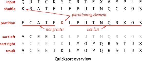
Quicksort is a divide-and-conquer method for sorting. It works by partitioning an array into two subarrays, then sorting the subarrays independently. Quicksort is complementary to mergesort: for mergesort, we break the array into two subarrays to be sorted and then combine the ordered subarrays to make the whole ordered array; for quicksort, we rearrange the array such that, when the two subarrays are sorted, the whole array is ordered. In the first instance, we do the two recursive calls before working on the whole array; in the second instance, we do the two recursive callsafter working on the whole array. For mergesort, the array is divided in half; for quicksort, the position of the partition depends on the contents of the array.
Algorithm 2.5 Quicksort
public class Quick
{
public static void sort(Comparable[] a)
{
StdRandom.shuffle(a); // Eliminate dependence on input.
sort(a, 0, a.length - 1);
}
private static void sort(Comparable[] a, int lo, int hi)
{
if (hi <= lo) return;
int j = partition(a, lo, hi); // Partition (see page 291).
sort(a, lo, j-1); // Sort left part a[lo .. j-1].
sort(a, j+1, hi); // Sort right part a[j+1 .. hi].
}
}
Quicksort is a recursive program that sorts a subarray a[lo..hi] by using a partition() method that puts a[j] into position and arranges the rest of the entries such that the recursive calls finish the sort.
The crux of the method is the partitioning process, which rearranges the array to make the following three conditions hold:
• The entry a[j] is in its final place in the array, for some j.
• No entry in a[lo] through a[j-1] is greater than a[j].
• No entry in a[j+1] through a[hi] is less than a[j].
We achieve a complete sort by partitioning, then recursively applying the method.
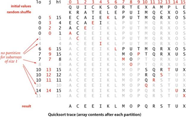
Because the partitioning process always fixes one item into its position, a formal proof by induction that the recursive method constitutes a proper sort is not difficult to develop: if the left subarray and the right subarray are both properly sorted, then the result array, made up of the left subarray (in order, with no entry larger than the partitioning item), the partitioning item, and the right subarray (in order, with no entry smaller that the partitioning item), is in order. ALGORITHM 2.5 is a recursive program that implements this idea. It is a randomized algorithm, because it randomly shuffles the array before sorting it. Our reason for doing so is to be able to predict (and depend upon) its performance characteristics, as discussed below.
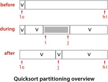
To complete the implementation, we need to implement the partitioning method. We use the following general strategy: First, we arbitrarily choose a[lo] to be the partitioning item—the one that will go into its final position. Next, we scan from the left end of the array until we find an entry greater than (or equal to) the partitioning item, and we scan from the right end of the array until we find an entry less than (or equal to) the partitioning item. The two items that stopped the scans are out of place in the final partitioned array, so we exchange them. Continuing in this way, we ensure that no array entries to the left of the left index i are greater than the partitioning item, and no array entries to the right of the right index j are less than the partitioning item. When the scan indices cross, all that we need to do to complete the partitioning process is to exchange the partitioning item a[lo] with the rightmost entry of the left subarray (a[j]) and return its index j.
There are several subtle issues with respect to implementing quicksort that are reflected in this code and worthy of mention, because each either can lead to incorrect code or can significantly impact performance. Next, we discuss several of these issues. Later in this section, we will consider three important higher-level algorithmic improvements.
Quicksort partitioning
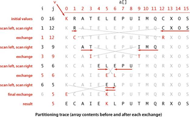
private static int partition(Comparable[] a, int lo, int hi)
{ // Partition into a[lo..i-1], a[i], a[i+1..hi].
int i = lo, j = hi+1; // left and right scan indices
Comparable v = a[lo]; // partitioning item
while (true)
{ // Scan right, scan left, check for scan complete, and exchange.
while (less(a[++i], v)) if (i == hi) break;
while (less(v, a[--j])) if (j == lo) break;
if (i >= j) break;
exch(a, i, j);
}
exch(a, lo, j); // Put v = a[j] into position
return j; // with a[lo..j-1] <= a[j] <= a[j+1..hi].
}
This code partitions on the item v in a[lo]. The main loop exits when the scan indices i and j cross. Within the loop, we increment i while a[i] is less than v and decrement j while a[j] is greater than v, then do an exchange to maintain the invariant property that no entries to the left of i are greater than v and no entries to the right of j are smaller than v. Once the indices meet, we complete the partitioning by exchanging a[lo] with a[j] (thus leaving the partitioning value in a[j]).
Partitioning in place
If we use an extra array, partitioning is easy to implement, but not so much easier that it is worth the extra cost of copying the partitioned version back into the original. A novice Java programmer might even create a new spare array within the recursive method, for each partition, which would drastically slow down the sort.
Staying in bounds
If the smallest item or the largest item in the array is the partitioning item, we have to take care that the pointers do not run off the left or right ends of the array, respectively. Our partition() implementation has explicit tests to guard against this circumstance. The test (j == lo) is redundant, since the partitioning item is at a[lo] and not less than itself. With a similar technique on the right it is not difficult to eliminate both tests (see EXERCISE 2.3.17).
Preserving randomness
The random shuffle puts the array in random order. Since it treats all items in the subarrays uniformly, ALGORITHM 2.5 has the property that its two subarrays are also in random order. This fact is crucial to the predictability of the algorithm’s running time. An alternate way to preserve randomness is to choose a random item for partitioning within partition().
Terminating the loop
Experienced programmers know to take special care to ensure that any loop must always terminate, and the partitioning loop for quicksort is no exception. Properly testing whether the pointers have crossed is a bit trickier than it might seem at first glance. A common error is to fail to take into account that the array might contain other items with the same key value as the partitioning item.
Handling items with keys equal to the partitioning item’s key
It is best to stop the left scan for items with keys greater than or equal to the partitioning item’s key and the right scan for items with key less than or equal to the partitioning item’s key, as in ALGORITHM 2.5. Even though this policy might seem to create unnecessary exchanges involving items with keys equal to the partitioning item’s key, it is crucial to avoiding quadratic running time in certain typical applications (see EXERCISE 2.3.11). Later, we discuss a better strategy for the case when the array contains a large number of items with equal keys.
Terminating the recursion
Experienced programmers also know to take special care to ensure that any recursive method must always terminate, and quicksort is again no exception. For instance, a common mistake in implementing quicksort involves not ensuring that one item is always put into position, then falling into an infinite recursive loop when the partitioning item happens to be the largest or smallest item in the array.
Performance characteristics
Quicksort has been subjected to very thorough mathematical analysis, so that we can make precise statements about its performance. The analysis has been validated through extensive empirical experience, and is a useful tool in tuning the algorithm for optimum performance.
The inner loop of quicksort (in the partitioning method) increments an index and compares an array entry against a fixed value. This simplicity is one factor that makes quicksort quick: it is hard to envision a shorter inner loop in a sorting algorithm. For example, mergesort and shellshort are typically slower than quicksort because they also do data movement within their inner loops.
The second factor that makes quicksort quick is that it uses few compares. Ultimately, the efficiency of the sort depends on how well the partitioning divides the array, which in turn depends on the value of the partitioning item’s key. Partitioning divides a large randomly ordered array into two smaller randomly ordered subarrays, but the actual split is equally likely (for distinct keys) to be anywhere in the array. Next, we consider the analysis of the algorithm, which allows us to see how this choice compares to the ideal choice.
The best case for quicksort is when each partitioning stage divides the array exactly in half. This circumstance would make the number of compares used by quicksort satisfy the divide-and-conquer recurrence CN = 2CN/2 + N. The 2CN/2 term covers the cost of sorting the two subarrays; the Nis the cost of examining each entry, using one partitioning index or the other. As in the proof of PROPOSITION F for mergesort, we know that this recurrence has the solution CN ~ N lg N. Although things do not always go this well, it is true that the partition falls in the middle on the average. Taking into account the precise probability of each partition position makes the recurrence more complicated and more difficult to solve, but the final result is similar. The proof of this result is the basis for our confidence in quicksort. If you are not mathematically inclined, you may wish to skip (and trust) it; if you are mathematically inclined, you may find it intriguing.
Proposition K. Quicksort uses ~ 2N ln N compares (and one-sixth that many exchanges) on the average to sort an array of length N with distinct keys.
Proof: Let CN be the average number of compares needed to sort N items with distinct values. We have C0 = C1 = 0 and for N > 1 we can write a recurrence relationship that directly mirrors the recursive program:
CN = N + 1 + (C0 + C1 + . . . + CN−2 + CN−1) / N + (CN−1 + CN−2 + . . . + C0)/N
The first term is the cost of partitioning (always N + 1), the second term is the average cost of sorting the left subarray (which is equally likely to be any size from 0 to N − 1), and the third term is the average cost for the right subarray (which is the same as for the left subarray). Multiplying by N and collecting terms transforms this equation to
NCN = N(N + 1) + 2(C0 + C1+ . . . +CN−2+CN−1)
Subtracting the same equation for N − 1 from this equation gives
NCN − (N − 1)CN−1 = 2N + 2CN−1
Rearranging terms and dividing by N(N + 1) leaves
CN/(N + 1) = CN−1/N + 2/(N + 1)
which telescopes to give the result
CN ~ 2 (N + 1)(1/3 + 1/4 + . . . + 1/(N + 1) )
The parenthesized quantity is the discrete estimate of the area under the curve 1/x from 3 to N + 1 and CN ~ 2N lnN by integration. Note that 2N ln N ≈ 1.39N lg N, so the average number of compares is only about 39 percent higher than in the best case.
A similar (but much more complicated) analysis is needed to establish the stated result for exchanges.
When keys may not be distinct, as is typical in practical applications, precise analysis is considerably more complicated, but it is not difficult to show that the average number of compares is no greater than CN, even when duplicate keys may be present (on page 296, we will look at a way toimprove quicksort in this case).
Despite its many assets, the basic quicksort program has one potential liability: it can be extremely inefficient if the partitions are unbalanced. For example, it could be the case that the first partition is on the smallest item, the second partition on the next smallest item, and so forth, so that the program will remove just one item for each call, leading to an excessive number of partitions of large subarrays. Avoiding this situation is the primary reason that we randomly shuffle the array before using quicksort. This action makes it so unlikely that bad partitions will happen consistently that we need not worry about the possibility.
Proposition L. Quicksort uses ~ N2/2 compares in the worst case, but random shuffling protects against this case.
Proof: By the argument just given, the number of compares used when one of the subarrays is empty for every partition is
N + (N − 1) + (N − 2) + . . . + 2 + 1 = (N + 1) N / 2
This behavior means not only that the time required will be quadratic but also that the space required to handle the recursion will be linear, which is unacceptable for large arrays. But (with quite a bit more work) it is possible to extend the analysis that we did for the average to find that the standard deviation of the number of compares is about .65 N, so the running time tends to the average as N grows and is unlikely to be far from the average. For example, even the rough estimate provided by Chebyshev’s inequality says that the probability that the running time is more than ten times the average for an array with a million elements is less than .00001 (and the true probability is far smaller). The probability that the running time for a large array is close to quadratic is so remote that we can safely ignore the possibility (see EXERCISE 2.3.10). For example, the probability that quicksort will use as many compares as insertion sort or selection sort when sorting a large array on your computer is much less than the probability that your computer will be struck by lightning during the sort!
IN SUMMARY, you can be sure that the running time of ALGORITHM 2.5 will be within a constant factor of 1.39N lg N whenever it is used to sort N items. The same is true of mergesort, but quicksort is typically faster because (even though it does 39 percent more compares) it does much less data movement. This mathematical assurance is probabilistic, but you can certainly rely upon it.
Algorithmic improvements
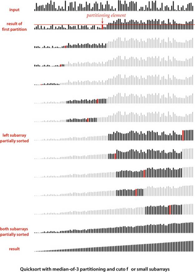
Quicksort was invented in 1960 by C. A. R. Hoare, and many people have studied and refined it since that time. It is tempting to try to develop ways to improve quicksort: a faster sorting algorithm is computer science’s “better mousetrap,” and quicksort is a venerable method that seems to invite tinkering. Almost from the moment Hoare first published the algorithm, people began proposing ways to improve the algorithm. Not all of these ideas are fully successful, because the algorithm is so well-balanced that the effects of improvements can be more than offset by unexpected side effects, but a few of them, which we now consider, are quite effective.
If your sort code is to be used a great many times or to sort a huge array (or, in particular, if it is to be used as a library sort that will be used to sort arrays of unknown characteristics), then it is worthwhile to consider the improvements that are discussed in the next few paragraphs. As noted, you need to run experiments to determine the effectiveness of these improvements and to determine the best choice of parameters for your implementation. Typically, improvements of 20 to 30 percent are available.
Cutoff to insertion sort
As with most recursive algorithms, an easy way to improve the performance of quicksort is based on the following two observations:
• Quicksort is slower than insertion sort for tiny subarrays.
• Being recursive, quicksort’s sort() is certain to call itself for tiny subarrays.
Accordingly, it pays to switch to insertion sort for tiny subarrays. A simple change to ALGORITHM 2.5 accomplishes this improvement: replace the statement
if (hi <= lo) return;
in sort() with a statement that invokes insertion sort for small subarrays:
if (hi <= lo + M) { Insertion.sort(a, lo, hi); return; }
The optimum value of the cutoff M is system-dependent, but any value between 5 and 15 is likely to work well in most situations (see EXERCISE 2.3.25).
Median-of-three partitioning
A second easy way to improve the performance of quicksort is to use the median of a small sample of items taken from the subarray as the partitioning item. Doing so will give a slightly better partition, but at the cost of computing the median. It turns out that most of the available improvement comes from choosing a sample of size 3 and then partitioning on the middle item (see EXERCISES 2.3.18 and 2.3.19). As a bonus, we can use the sample items as sentinels at the ends of the array and remove both array bounds tests in partition().
Entropy-optimal sorting
Arrays with large numbers of duplicate keys arise frequently in applications. For example, we might wish to sort a large personnel file by year of birth, or perhaps to separate females from males. In such situations, the quicksort implementation that we have considered has acceptable performance, but it can be substantially improved. For example, a subarray that consists solely of items that are equal (just one key value) does not need to be processed further, but our implementation keeps partitioning down to small subarrays. In a situation where there are large numbers of duplicate keys in the input array, the recursive nature of quicksort ensures that subarrays consisting solely of items with keys that are equal will occur often. There is potential for significant improvement, from the linearithmic-time performance of the implementations seen so far to linear-time performance.
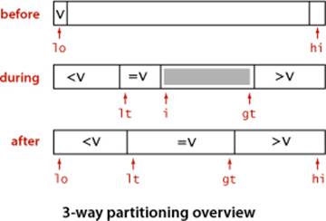
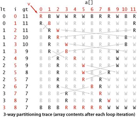
One straightforward idea is to partition the array into three parts, one each for items with keys smaller than, equal to, and larger than the partitioning item’s key. Accomplishing this partitioning is more complicated than the 2-way partitioning that we have been using, and various different methods have been suggested for the task. It was a classical programming exercise popularized by E. W. Dijkstra as the Dutch National Flag problem, because it is like sorting an array with three possible key values, which might correspond to the three colors on the flag.
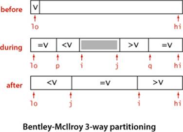
Dijkstra’s solution to this problem leads to the remarkably simple partition code shown on the next page. It is based on a single left-to-right pass through the array that maintains a pointer lt such that a[lo..lt-1] is less than v, a pointer gt such that a[gt+1, hi] is greater than v, and a pointer i such that a[lt..i-1] are equal to v and a[i..gt] are not yet examined. Starting with i equal to lo, we process a[i] using the 3-way comparison given by the Comparable interface (instead of using less()) to directly handle the three possible cases:
• a[i] less than v: exchange a[lt] with a[i] and increment both lt and i
• a[i] greater than v: exchange a[i] with a[gt] and decrement gt
• a[i] equal to v: increment i
Each of these operations both maintains the invariant and decreases the value of gt-i (so that the loop terminates). Furthermore, every item encountered leads to an exchange except for those items with keys equal to the partitioning item’s key.
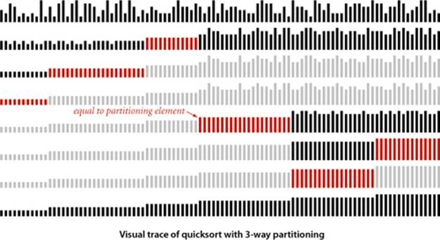
Though this code was developed not long after quicksort in the 1970s, it fell out of favor because it uses many more exchanges than the standard 2-way partitioning method for the common case when the number of duplicate keys in the array is not high. In the 1990s J. Bentley and D. McIlroy developed a clever implementation that overcomes this problem (see EXERCISE 2.3.22), and observed that 3-way partitioning makes quicksort asymptotically faster than mergesort and other methods in practical situations involving large numbers of equal keys. Later, J. Bentley and R. Sedgewick developed a proof of this fact, which we discuss next.
But we proved that mergesort is optimal. How have we defeated that lower bound? The answer to this question is that PROPOSITION I in SECTION 2.2 addresses worst-case performance over all possible inputs, while now we are looking at worst-case performance with some information about the key values at hand. Mergesort does not guarantee optimal performance for any given distribution of duplicates in the input: for example, mergesort is linearithmic for a randomly ordered array that has only a constant number of distinct key values, but quicksort with 3-way partitioning is linear for such an array. Indeed, by examining the visual trace above, you can see that N times the number of key values is a conservative bound on the running time.
Quicksort with 3-way partitioning
public class Quick3way
{
private static void sort(Comparable[] a, int lo, int hi)
{ // See page 289 for public sort() that calls this method.
if (hi <= lo) return;
int lt = lo, i = lo+1, gt = hi;
Comparable v = a[lo];
while (i <= gt)
{
int cmp = a[i].compareTo(v);
if (cmp < 0) exch(a, lt++, i++);
else if (cmp > 0) exch(a, i, gt--);
else i++;
} // Now a[lo..lt-1] < v = a[lt..gt] < a[gt+1..hi].
sort(a, lo, lt - 1);
sort(a, gt + 1, hi);
}
}
This sort code partitions to put keys equal to the partitioning element in place and thus does not have to include those keys in the subarrays for the recursive calls. It is far more efficient than the standard quicksort implementation for arrays with large numbers of duplicate keys (see text).
The analysis that makes these notions precise takes the distribution of key values into account. Given N keys with k distinct key values, for each i from 1 to k define fi to be frequency of occurrence of the ith key value and pi to be fi / N, the probability that the ith key value is found when a random entry of the array is sampled. The Shannon entropy of the keys (a classic measure of their information content) is defined as
H = − (p1 lg p1 + p2 lg p2 + . . . + pk lg pk)
Given any array of items to be sorted, we can calculate its entropy by counting the frequency of each key value. Remarkably, we can also derive from the entropy both a lower bound on the number of compares and an upper bound on the number of compares used by quicksort with 3-way partitioning.
Proposition M. No compare-based sorting algorithm can guarantee to sort N items with fewer than NH − N compares, where H is the Shannon entropy, defined from the frequencies of key values.
Proof sketch: This result follows from a (relatively easy) generalization of the lower bound proof of PROPOSITION I in SECTION 2.2.
Proposition N. Quicksort with 3-way partitioning uses ~ (2ln 2) N H compares to sort N items, where H is the Shannon entropy, defined from the frequencies of key values.
Proof sketch: This result follows from a (relatively difficult) generalization of the average-case analysis of quicksort in PROPOSITION K. As with distinct keys, this costs about 39 percent more than the optimum (but within a constant factor).
Note that H = lg N when the keys are all distinct (all the probabilities are 1/N), which is consistent with PROPOSITION I in SECTION 2.2 and PROPOSITION K. The worst case for 3-way partitioning happens when the keys are distinct; when duplicate keys are present, it can do much better than mergesort. More important, these two properties together imply that quicksort with 3-way partitioning is entropy-optimal, in the sense that the average number of compares used by the best possible compare-based sorting algorithm and the average number of compares used by 3-way quicksort are within a constant factor of one another, for any given distribution of input key values.
As with standard quicksort, the running time tends to the average as the array size grows, and large deviations from the average are extremely unlikely, so that you can depend on 3-way quicksort’s running time to be proportional to N times the entropy of the distribution of input key values. This property of the algorithm is important in practice because it reduces the time of the sort from linearithmic to linear for arrays with large numbers of duplicate keys. The order of the keys is immaterial, because the algorithm shuffles them to protect against the worst case. The distribution of keys defines the entropy and no compare-based algorithm can use fewer compares than defined by the entropy. This ability to adapt to duplicates in the input makes 3-way quicksort the algorithm of choice for a library sort—clients that sort arrays containing large numbers of duplicate keys are not unusual.
A CAREFULLY TUNED VERSION of quicksort is likely to run significantly faster on most computers for most applications than will any other compare-based sorting method. Quicksort is widely used throughout today’s computational infrastructure because the mathematical models that we have discussed suggest that it will outperform other methods in practical applications, and extensive experiments and experience over the past several decades have validated that conclusion.
We will see in CHAPTER 5 that this is not quite the end of the story in the development of sorting algorithms, because it is possible to develop algorithms that do not use compares at all! But a version of quicksort turns out to be best in that situation, as well.
Q & A
Q. Is there some way to just divide the array into two halves, rather than letting the partitioning element fall where it may?
A. That is a question that stumped experts for over a decade. It is tantamount to finding the median key value in the array and then partitioning on that value. We discuss the problem of finding the median on page 346. It is possible to do so in linear time, but the cost of doing so with known algorithms (which are based on quicksort partitioning!) far exceeds the 39 percent savings available from splitting the array into equal parts.
Q. Randomly shuffling the array seems to take a significant fraction of the total time for the sort. Is doing so really worthwhile?
A. Yes. It protects against the worst case and makes the running time predictable. Hoare proposed this approach when he presented the algorithm in 1960—it is a prototypical (and among the first) randomized algorithm.
Q. Why all the focus on items with equal keys?
A. The issue directly impacts performance in practical situations. It was overlooked by many for decades, with the result that some older implementations of quicksort take quadratic time for arrays with large numbers of items with equal keys, which certainly do arise in applications. Better implementations such as ALGORITHM 2.5 take linearithmic time for such arrays, but improving that to linear-time as in the entropy-optimal sort at the end of this section is worthwhile in many situations.
Exercises
2.3.1 Show, in the style of the trace given with partition(), how that method partitions the array E A S Y Q U E S T I O N.
2.3.2 Show, in the style of the quicksort trace given in this section, how quicksort sorts the array E A S Y Q U E S T I O N (for the purposes of this exercise, ignore the initial shuffle).
2.3.3 What is the maximum number of times during the execution of Quick.sort() that the largest item can be exchanged, for an array of length N?
2.3.4 Suppose that the initial random shuffle is omitted. Give six arrays of ten elements for which Quick.sort() uses the worst-case number of compares.
2.3.5 Give a code fragment that sorts an array that is known to consist of items having just two distinct keys.
2.3.6 Write a program to compute the exact value of CN, and compare the exact value with the approximation 2N ln N, for N = 100, 1,000, and 10,000.
2.3.7 Find the expected number of subarrays of size 0, 1, and 2 when quicksort is used to sort an array of N items with distinct keys. If you are mathematically inclined, do the math; if not, run some experiments to develop hypotheses.
2.3.8 About how many compares will Quick.sort() make when sorting an array of N items that are all equal?
2.3.9 Explain what happens when Quick.sort() is run on an array having items with just two distinct keys, and then explain what happens when it is run on an array having just three distinct keys.
2.3.10 Chebyshev’s inequality says that the probability that a random variable is more than k standard deviations away from the mean is less than 1/k2. For N = 1 million, use Chebyshev’s inequality to bound the probability that the number of compares used by quicksort is more than 100 billion (.1 N2).
2.3.11 Suppose that we scan over items with keys equal to the partitioning item’s key instead of stopping the scans when we encounter them. Show that the running time of this version of quicksort is quadratic for all arrays with just a constant number of distinct keys.
2.3.12 Show, in the style of the trace given with the code, how the the 3-way quicksort first partitions the array B A B A B A B A C A D A B R A.
2.3.13 What is the recursive depth of quicksort, in the best, worst, and average cases? This is the size of the stack that the system needs to keep track of the recursive calls. See EXERCISE 2.3.20 for a way to guarantee that the recursive depth is logarithmic in the worst case.
2.3.14 Prove that when running quicksort on an array with N distinct items, the probability of comparing the ith and jth smallest items is 2/(j − i − 1). Then use this result to prove PROPOSITION K.
Creative Problems
2.3.15 Nuts and bolts. (G. J. E. Rawlins) You have a mixed pile of N nuts and N bolts and need to quickly find the corresponding pairs of nuts and bolts. Each nut matches exactly one bolt, and each bolt matches exactly one nut. By fitting a nut and bolt together, you can see which is bigger, but it is not possible to directly compare two nuts or two bolts. Give an efficient method for solving the problem.
2.3.16 Best case. Write a program that produces a best-case array (with no duplicates) for sort() in ALGORITHM 2.5: an array of N items with distinct keys having the property that every partition will produce subarrays that differ in size by at most 1 (the same subarray sizes that would happen for an array of N equal keys). (For the purposes of this exercise, ignore the initial shuffle.)
The following exercises describe variants of quicksort. Each of them calls for an implementation, but naturally you will also want to use SortCompare for experiments to evaluate the effectiveness of each suggested modification.
2.3.17 Sentinels. Modify the code in ALGORITHM 2.5 to remove both bounds checks in the inner while loops. The test against the left end of the subarray is redundant since the partitioning item acts as a sentinel (v is never less than a[lo]). To enable removal of the other test, put an item whose key is the largest in the whole array into a[length-1] just after the shuffle. This item will never move (except possibly to be swapped with an item having the same key) and will serve as a sentinel in all subarrays involving the end of the array. Note: For a subarray that does not involve the end of the array, the leftmost entry to its right serves as a sentinel for the right end of the subarray.
2.3.18 Median-of-3 partitioning. Add median-of-3 partitioning to quicksort, as described in the text (see page 296). Run doubling tests to determine the effectiveness of the change.
2.3.19 Median-of-5 partitioning. Implement a quicksort based on partitioning on the median of a random sample of five items from the subarray. Put the items of the sample at the appropriate ends of the array so that only the median participates in partitioning. Run doubling tests to determine the effectiveness of the change, in comparison both to the standard algorithm and to median-of-3 partitioning (see the previous exercise). Extra credit: Devise a median-of-5 algorithm that uses fewer than seven compares on any input.
2.3.20 Nonrecursive quicksort. Implement a nonrecursive version of quicksort based on a main loop where a subarray is popped from a stack to be partitioned, and the resulting subarrays are pushed onto the stack. Note: Push the larger of the subarrays onto the stack first, which guarantees that the stack will have at most lg N entries.
2.3.21 Lower bound for sorting with equal keys. Complete the first part of the proof of PROPOSITION M by following the logic in the proof of PROPOSITION I and using the observation that there are N! / f1!f2! . . . fk! different ways to arrange keys with k different values, where the i th value appears with frequency fi (= Npi, in the notation of PROPOSITION M), with f1+ . . . +fk = N.
2.3.22 Fast 3-way partitioning. (J. Bentley and D. McIlroy) Implement an entropy-optimal sort based on keeping items with equal keys at both the left and right ends of the subarray. Maintain indices p and q such that a[lo..p-1] and a[q+1..hi] are all equal to a[lo], an index i such that a[p..i-1] are all less than a[lo], and an index j such that a[j+1..q] are all greater than a[lo]. Add to the inner partitioning loop code to swap a[i] with a[p] (and increment p) if it is equal to v and to swap a[j] with a[q] (and decrement q) if it is equal to v before the usual comparisons of a[i] and a[j] with v. After the partitioning loop has terminated, add code to swap the items with equal keys into position. Note: This code complements the code given in the text, in the sense that it does extra swaps for keys equal to the partitioning item’s key, while the code in the text does extra swaps for keys that are notequal to the partitioning item’s key.
2.3.23 Turkey’s ninther. Add to your implementation from EXERCISE 2.3.22 code to use the Tukey ninther to compute the partitioning item—choose three sets of three items, take the median of each, then use the median of the three medians as the partitioning item. Also, add a cutoff to insertion sort for small subarrays.
2.3.24 Samplesort. (W. Frazer and A. McKellar) Implement a quicksort based on using a sample of size 2k − 1. First, sort the sample, then arrange to have the recursive routine partition on the median of the sample and to move the two halves of the rest of the sample to each subarray, such that they can be used in the subarrays, without having to be sorted again. This algorithm is called samplesort.
Experiments
2.3.25 Cutoff to insertion sort. Implement quicksort with a cutoff to insertion sort for subarrays with less than M elements, and empirically determine the value of M for which quicksort runs fastest in your computing environment to sort random arrays of N doubles, for N = 103, 104, 105, and 106. Plot average running times for M from 0 to 30 for each value of M. Note: You need to add a three-argument sort() method to ALGORITHM 2.2 for sorting subarrays such that the call Insertion.sort(a, lo, hi) sorts the subarray a[lo..hi].
2.3.26 Subarray sizes. Write a program that plots a histogram of the subarray sizes left for insertion sort when you run quicksort for an array of size N with a cutoff for subarrays of size less than M. Run your program for M=10, 20, and 50 and N = 105.
2.3.27 Ignore small subarrays. Run experiments to compare the following strategy for dealing with small subarrays with the approach described in EXERCISE 2.3.25: Simply ignore the small subarrays in quicksort, then run a single insertion sort after the quicksort completes. Note: You may be able to estimate the size of your computer’s cache memory with these experiments, as the performance of this method is likely to degrade when the array does not fit in the cache.
2.3.28 Recursion depth. Run empirical studies to determine the average recursive depth used by quicksort with cutoff for arrays of size M, when sorting arrays of N distinct elements, for M=10, 20, and 50 and N = 103, 104, 105, and 106.
2.3.29 Randomization. Run empirical studies to compare the effectiveness of the strategy of choosing a random partitioning item with the strategy of initially randomizing the array (as in the text). Use a cutoff for arrays of size M, and sort arrays of N distinct elements, for M=10, 20, and 50 and N = 103, 104, 105, and 106.
2.3.30 Corner cases. Test quicksort on large nonrandom arrays of the kind described in EXERCISES 2.1.35 and 2.1.36 both with and without the initial random shuffle. How does shuffling affect its performance for these arrays?
2.3.31 Histogram of running times. Write a program that takes command-line arguments N and T, does T trials of the experiment of running quicksort on an array of N random Double values, and plots a histogram of the observed running times. Run your program for N = 103, 104, 105, and 106, with T as large as you can afford to make the curves smooth. Your main challenge for this exercise is to appropriately scale the experimental results.
All materials on the site are licensed Creative Commons Attribution-Sharealike 3.0 Unported CC BY-SA 3.0 & GNU Free Documentation License (GFDL)
If you are the copyright holder of any material contained on our site and intend to remove it, please contact our site administrator for approval.
© 2016-2026 All site design rights belong to S.Y.A.