Algorithms (2014)
Four. Graphs
4.1 Undirected Graphs 518
4.2 Directed Graphs 566
4.3 Minimum Spanning Trees 604
4.4 Shortest Paths 638
Pairwise connections between items play a critical role in a vast array of computational applications. The relationships implied by these connections lead immediately to a host of natural questions: Is there a way to connect one item to another by following the connections? How many other items are connected to a given item? What is the shortest chain of connections between this item and this other item?
To model such situations, we use abstract mathematical objects called graphs. In this chapter, we examine basic properties of graphs in detail, setting the stage for us to study a variety of algorithms that are useful for answering questions of the type just posed. These algorithms serve as the basis for attacking problems in important applications whose solution we could not even contemplate without good algorithmic technology.
Graph theory, a major branch of mathematics, has been studied intensively for hundreds of years. Many important and useful properties of graphs have been discovered, many important algorithms have been developed, and many difficult problems are still actively being studied. In this chapter, we introduce a variety of fundamental graph algorithms that are important in diverse applications.
Like so many of the other problem domains that we have studied, the algorithmic investigation of graphs is relatively recent. Although a few of the fundamental algorithms are centuries old, the majority of the interesting ones have been discovered within the last several decades and have benefited from the emergence of the algorithmic technology that we have been studying. Even the simplest graph algorithms lead to useful computer programs, and the nontrivial algorithms that we examine are among the most elegant and interesting algorithms known.
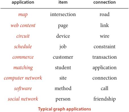
To illustrate the diversity of applications that involve graph processing, we begin our exploration of algorithms in this fertile area by introducing several examples.
Maps
A person who is planning a trip may need to answer questions such as “What is the shortest route from Providence to Princeton?” A seasoned traveler who has experienced traffic delays on the shortest route may ask the question “What is the fastest way to get from Providence to Princeton?” To answer such questions, we process information about connections (roads) between items (intersections).
Web content
When we browse the web, we encounter pages that contain references (links) to other pages and we move from page to page by clicking on the links. The entire web is a graph, where the items are pages and the connections are links. Graph-processing algorithms are essential components of the search engines that help us locate information on the web.
Circuits
An electric circuit comprises devices such as transistors, resistors, and capacitors that are intricately wired together. We use computers to control machines that make circuits and to check that the circuits perform desired functions. We need to answer simple questions such as “Is a short-circuit present?” as well as complicated questions such as “Can we lay out this circuit on a chip without making any wires cross?” The answer to the first question depends on only the properties of the connections (wires), whereas the answer to the second question requires detailed information about the wires, the devices that those wires connect, and the physical constraints of the chip.
Schedules
A manufacturing process requires a variety of jobs to be performed, under a set of constraints that specify that certain jobs cannot be started until certain other jobs have been completed. How do we schedule the jobs such that we both respect the given constraints and complete the whole process in the least amount of time?
Commerce
Retailers and financial institutions track buy/sell orders in a market. A connection in this situation represents the transfer of cash and goods between an institution and a customer. Knowledge of the nature of the connection structure in this instance may enhance our understanding of the nature of the market.
Matching
Students apply for positions in selective institutions such as social clubs, universities, or medical schools. Items correspond to the students and the institutions; connections correspond to the applications. We want to discover methods for matching interested students with available positions.
Computer networks
A computer network consists of interconnected sites that send, forward, and receive messages of various types. We are interested in knowing about the nature of the interconnection structure because we want to lay wires and build switches that can handle the traffic efficiently.
Software
A compiler builds graphs to represent relationships among modules in a large software system. The items are the various classes or modules that comprise the system; connections are associated either with the possibility that a method in one class might call another (static analysis) or with actual calls while the system is in operation (dynamic analysis). We need to analyze the graph to determine how best to allocate resources to the program most efficiently.
Social networks
When you use a social network, you build explicit connections with your friends. Items correspond to people; connections are to friends or followers. Understanding the properties of these networks is a modern graph-processing applications of intense interest not just to companies that support such networks, but also in politics, diplomacy, entertainment, education, marketing, and many other domains.
THESE EXAMPLES INDICATE THE RANGE OF APPLICATIONS for which graphs are the appropriate abstraction and also the range of computational problems that we might encounter when we work with graphs. Thousands of such problems have been studied, but many problems can be addressed in the context of one of several basic graph models—we will study the most important ones in this chapter. In practical applications, it is common for the volume of data involved to be truly huge, so that efficient algorithms make the difference between whether or not a solution is at all feasible.
To organize the presentation, we progress through the four most important types of graph models: undirected graphs (with simple connections), digraphs (where the direction of each connection is significant), edge-weighted graphs (where each connection has an associated weight), and edge-weighted digraphs (where each connection has both a direction and a weight).
4.1 Undirected Graphs
OUR STARTING POINT is the study of graph models where edges are nothing more than connections between vertices. We use the term undirected graph in contexts where we need to distinguish this model from other models (such as the title of this section), but, since this is the simplest model, we start with the following definition:
Definition. A graph is a set of vertices and a collection of edges that each connect a pair of vertices.
Vertex names are not important to the definition, but we need a way to refer to vertices. By convention, we use the names 0 through V−1 for the vertices in a V-vertex graph. The main reason that we choose this system is to make it easy to write code that efficiently accesses information corresponding to each vertex, using array indexing. It is not difficult to use a symbol table to establish a 1-1 mapping to associate V arbitrary vertex names with the V integers between 0 and V−1 (see page 548), so the convenience of using indices as vertex names comes without loss of generality (and without much loss of efficiency). We use the notation v-w to refer to an edge that connects v and w; the notation w-v is an alternate way to refer to the same edge.
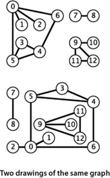
We draw a graph with circles for the vertices and lines connecting them for the edges. A drawing gives us intuition about the structure of the graph; but this intuition can be misleading, because the graph is defined independently of the drawing. For example, the two drawings at left represent the same graph, because the graph is nothing more than its (unordered) set of vertices and its (unordered) collection of edges (vertex pairs).
Anomalies
Our definition allows two simple anomalies:
• A self-loop is an edge that connects a vertex to itself.
• Two edges that connect the same pair of vertices are parallel.
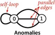
Mathematicians sometimes refer to graphs with parallel edges as multigraphs and graphs with no parallel edges or self-loops as simple graphs. Typically, our implementations allow self-loops and parallel edges (because they arise in applications), but we do not include them in examples. Thus, we can refer to every edge just by naming the two vertices it connects.
Glossary
A substantial amount of nomenclature is associated with graphs. Most of the terms have straightforward definitions, and, for reference, we consider them in one place: here.
When there is an edge connecting two vertices, we say that the vertices are adjacent to one another and that the edge is incident to both vertices. The degree of a vertex is the number of edges incident to it. A subgraph is a subset of a graph’s edges (and associated vertices) that constitutes a graph. Many computational tasks involve identifying subgraphs of various types. Of particular interest are edges that take us through a sequence of vertices in a graph.
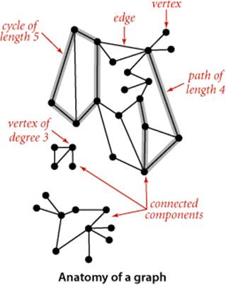
Definition. A path in a graph is a sequence of vertices connected by edges. A simple path is one with no repeated vertices. A cycle is a path with at least one edge whose first and last vertices are the same. A simple cycle is a cycle with no repeated edges or vertices (except the requisite repetition of the first and last vertices). The length of a path or a cycle is its number of edges.
Most often, we work with simple cycles and simple paths and drop the simple modifer; when we want to allow repeated vertices, we refer to general paths and cycles. We say that one vertex is connected to another if there exists a path that contains both of them. We use notation like u-v-w-x to represent a path from u to x and u-v-w-x-u to represent a cycle from u to v to w to x and back to u again. Several of the algorithms that we consider find paths and cycles. Moreover, paths and cycles lead us to consider the structural properties of a graph as a whole:
Definition. A graph is connected if there is a path from every vertex to every other vertex in the graph. A graph that is not connected consists of a set of connected components, which are maximal connected subgraphs.
Intuitively, if the vertices were physical objects, such as knots or beads, and the edges were physical connections, such as strings or wires, a connected graph would stay in one piece if picked up by any vertex, and a graph that is not connected comprises two or more such pieces. Generally, processing a graph necessitates processing the connected components one at a time.
An acyclic graph is a graph with no cycles. Several of the algorithms that we consider are concerned with finding acyclic subgraphs of a given graph that satisfy certain properties. We need additional terminology to refer to these structures:
Definition. A tree is an acyclic connected graph. A disjoint set of trees is called a forest. A spanning tree of a connected graph is a subgraph that contains all of that graph’s vertices and is a single tree. A spanning forest of a graph is the union of spanning trees of its connected components.
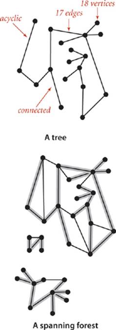
This definition of tree is quite general: with suitable refinements it embraces the trees that we typically use to model program behavior (function-call hierarchies) and data structures (BSTs, 2-3 trees, and so forth). Mathematical properties of trees are well-studied and intuitive, so we state them without proof. For example, a graph G with V vertices is a tree if and only if it satisfies any of the following five conditions:
• G has V−1 edges and no cycles.
• G has V−1 edges and is connected.
• G is connected, but removing any edge disconnects it.
• G is acyclic, but adding any edge creates a cycle.
• Exactly one simple path connects each pair of vertices in G.
Several of the algorithms that we consider find spanning trees and forests, and these properties play an important role in their analysis and implementation.
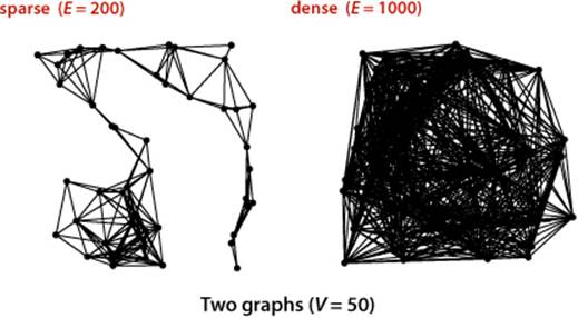
The density of a graph is the proportion of possible pairs of vertices that are connected by edges. A sparse graph has relatively few of the possible edges present; a dense graph has relatively few of the possible edges missing. Generally, we think of a graph as being sparse if its number of different edges is within a small constant factor of V and as being dense otherwise. This rule of thumb leaves a gray area (when the number of edges is, say, ~ c V3/2) but the distinction between sparse and dense is typically very clear in applications. The applications that we consider nearly always involve sparse graphs.
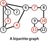
A bipartite graph is a graph whose vertices we can divide into two sets such that all edges connect a vertex in one set with a vertex in the other set. The figure at right gives an example of a bipartite graph, where one set of vertices is colored red and the other set of vertices is colored black. Bipartite graphs arise in a natural way in many situations, one of which we will consider in detail at the end of this section.
WITH THESE PREPARATIONS, we are ready to move on to consider graph-processing algorithms. We begin by considering an API and implementation for a graph data type, then we consider classic algorithms for searching graphs and for identifying connected components. To conclude the section, we consider real-world applications where vertex names need not be integers and graphs may have huge numbers of vertices and edges.
Undirected graph data type
Our starting point for developing graph-processing algorithms is an API that defines the fundamental graph operations. This scheme allows us to address graph-processing tasks ranging from elementary maintenance operations to sophisticated solutions of difficult problems.
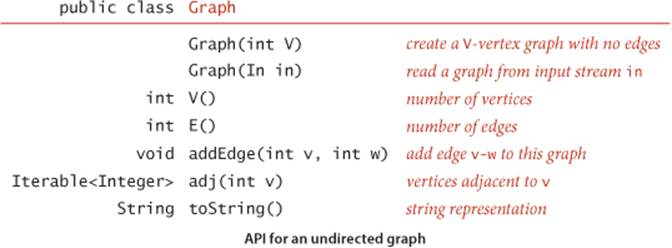
This API contains two constructors, methods to return the number of vertices and edges, a method to add an edge, a toString() method, and a method adj() that allows client code to iterate through the vertices adjacent to a given vertex (the order of iteration is not specified). Remarkably, we can build all of the algorithms that we consider in this section on the basic abstraction embodied in adj().
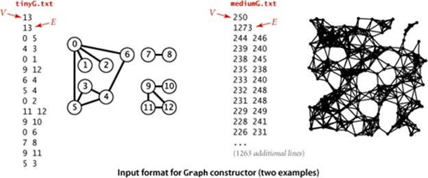
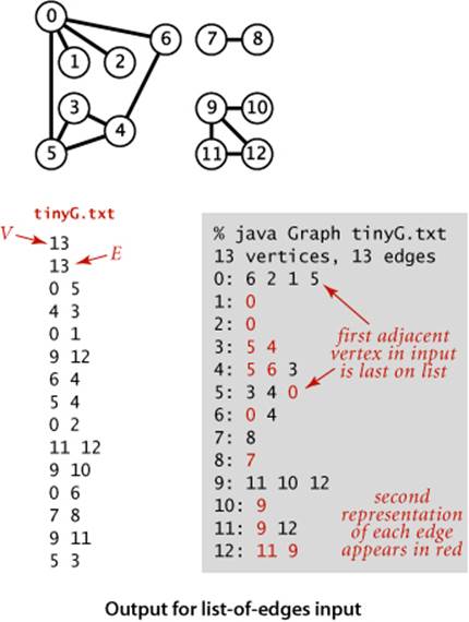
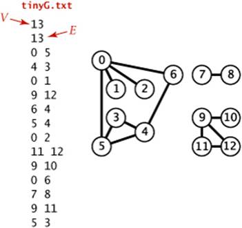
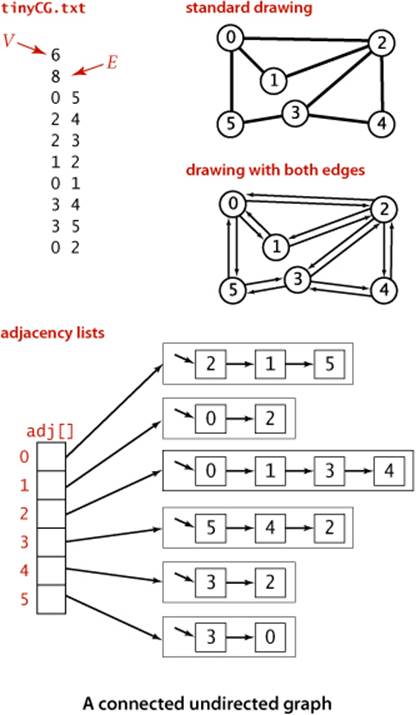
The second constructor assumes an input format consisting of 2E + 2 integer values: V, then E, then E pairs of values between 0 and V−1, each pair denoting an edge. As examples, we use the two graphs tinyG.txt and mediumG.txt that are depicted below.
Several examples of Graph client code are shown in the table on the facing page.
Representation alternatives
The next decision that we face in graph processing is which graph representation (data structure) to use to implement this API. We have two basic requirements:
• We must have the space to accommodate the types of graphs that we are likely to encounter in applications.
• We want to develop time-efficient implementations of Graph instance methods—the basic methods that we need to develop graph-processing clients.
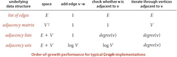
These requirements are a bit vague, but they are still helpful in choosing among the three data structures that immediately suggest themselves for representing graphs:
• An adjacency matrix, where we maintain a V-by-V boolean array, with the entry in row v and column w defined to be true if there is an edge in the graph that connects vertex v and vertex w in the graph, and to be false otherwise. This representation fails on the first count—graphs with millions of vertices are common and the space cost for the V2 boolean values needed is prohibitive.
• An array of edges, using an Edge class with two instance variables of type int. This direct representation is simple, but it fails on the second count—implementing adj() would involve examining all the edges in the graph.
• An array of adjacency lists, where we maintain a vertex-indexed array of lists of the vertices adjacent to each vertex. This data structure satisfies both requirements for typical applications and is the one that we will use throughout this chapter.
Beyond these performance objectives, a detailed examination reveals other considerations that can be important in some applications. For example, allowing parallel edges precludes the use of an adjacency matrix, since the adjacency matrix has no way to represent them.
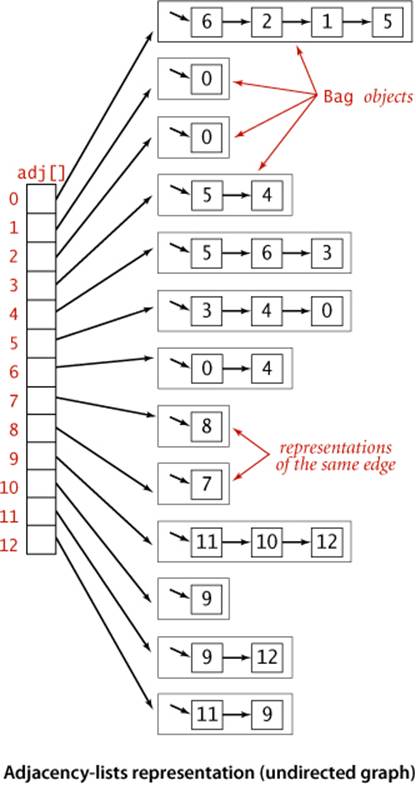
Adjacency-lists data structure
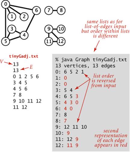
The standard graph representation for graphs that are not dense is called the adjacency-lists data structure, where we keep track of all the vertices adjacent to each vertex on a linked list that is associated with that vertex. We maintain an array of lists so that, given a vertex, we can immediately access its list. To implement lists, we use our Bag ADT from SECTION 1.3 with a linked-list implementation, so that we can add new edges in constant time and iterate through adjacent vertices in constant time per adjacent vertex. The Graph implementation on page 526 is based on this approach, and the figure on the facing page depicts the data structures built by this code for tinyG.txt. To add an edge connecting v and w, we add w to v’s adjacency list and v to w’s adjacency list. Thus, each edge appears twice in the data structure. This Graph implementation achieves the following performance characteristics:
• Space usage proportional to V + E
• Constant time to add an edge
• Time proportional to the degree of v to iterate through vertices adjacent to v (constant time per adjacent vertex processed)
These characteristics are optimal for this set of operations, which suffice for the graph-processing applications that we consider. Parallel edges and self-loops are allowed (we do not check for them). Note: It is important to realize that the order in which edges are added to the graph determines the order in which vertices appear in the array of adjacency lists built by Graph. Many different arrays of adjacency lists can represent the same graph. When using the constructor that reads edges from an input stream, this means that the input format and the order in which edges are specified in the file determine the order in which vertices appear in the array of adjacency lists built by Graph. Since our algorithms use adj() and process all adjacent vertices without regard to the order in which they appear in the lists, this difference does not affect their correctness, but it is important to bear it in mind when debugging or following traces. To facilitate these activities, we assume that Graph has a test client that reads a graph from the input stream named as command-line argument and then prints it (relying on the toString() implementation on page 523) to show the order in which vertices appear in adjacency lists, which is the order in which algorithms process them (see EXERCISE 4.1.7).
Graph data type
public class Graph
{
private final int V; // number of vertices
private int E; // number of edges
private Bag<Integer>[] adj; // adjacency lists
public Graph(int V)
{
this.V = V; this.E = 0;
adj = (Bag<Integer>[]) new Bag[V]; // Create array of lists.
for (int v = 0; v < V; v++) // Initialize all lists
adj[v] = new Bag<Integer>(); // to empty.
}
public Graph(In in)
{
this(in.readInt()); // Read V and construct this graph.
int E = in.readInt(); // Read E.
for (int i = 0; i < E; i++)
{ // Add an edge.
int v = in.readInt(); // Read a vertex,
int w = in.readInt(); // read another vertex,
addEdge(v, w); // and add edge connecting them.
}
}
public int V() { return V; }
public int E() { return E; }
public void addEdge(int v, int w)
{
adj[v].add(w); // Add w to v's list.
adj[w].add(v); // Add v to w's list.
E++;
}
public Iterable<Integer> adj(int v)
{ return adj[v]; }
}
This Graph implementation maintains a vertex-indexed array of lists of integers. Every edge appears twice: if an edge connects v and w, then w appears in v’s list and v appears in w’s list. The second constructor reads a graph from an input stream, in the format V followed by E followed by a list of pairs of int values between 0 and V−1. See page 523 for toString().
IT IS CERTAINLY REASONABLE to contemplate other operations that might be useful in applications, and to consider methods for
• Adding a vertex
• Deleting a vertex
One way to handle such operations is to expand the API and use a symbol table (ST) instead of a vertex-indexed array (with this change we also do not need our convention that vertex names be integer indices). We might also consider methods for
• Deleting an edge
• Checking whether the graph contains the edge v-w
To implement these two operations (and disallow parallel edges) we might use a SET instead of a Bag for adjacency lists. We refer to this alternative as an adjacency set representation. We do not use either of these two alternatives in this book for several reasons:
• Our clients do not need to add vertices, delete vertices and edges, or check whether an edge exists.
• When clients do need these operations, they typically are invoked infrequently or for short adjacency lists, so an easy option is to use a brute-force implementation that iterates through an adjacency list.
• The SET and ST representations slightly complicate algorithm implementation code, diverting attention from the algorithms themselves.
• A performance penalty of log V is involved in some situations.
It is not difficult to adapt our algorithms to accommodate other designs (for example disallowing parallel edges or self-loops) without undue performance penalties. The table below summarizes performance characteristics of the alternatives that we have mentioned. Typical applications process huge sparse graphs, so we use the adjacency-lists representation throughout.
Design pattern for graph processing
Since we consider a large number of graph-processing algorithms, our initial design goal is to decouple our implementations from the graph representation. To do so, we develop, for each given task, a task-specific class so that clients can create objects to perform the task. Generally, the constructor does some preprocessing to build data structures so as to efficiently respond to client queries. A typical client program builds a graph, passes that graph to an algorithm implementation class (as argument to a constructor), and then calls client query methods to learn various properties of the graph. As a warmup, consider this API:
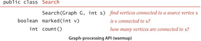
We use the term source to distinguish the vertex provided as argument to the constructor from the other vertices in the graph. In this API, the job of the constructor is to find the vertices in the graph that are connected to the source. Then client code calls the instance methods marked() and count()to learn characteristics of the graph. The name marked() refers to an approach used by the basic algorithms that we consider throughout this chapter: they follow paths from the source to other vertices in the graph, marking each vertex encountered. The example client TestSearch shown on the facing page takes an input stream name and a source vertex number from the command line, reads a graph from the input stream (using the second Graph constructor), builds a Search object for the given graph and source, and uses marked() to print the vertices in that graph that are connected to the source. It also calls count() and prints whether or not the graph is connected (the graph is connected if and only if the search marked all of its vertices).
WE HAVE ALREADY SEEN one way to implement the Search API: the union-find algorithms of CHAPTER 1. The constructor can build a UF object, do a union() operation for each of the graph’s edges, and implement marked(v) by calling connected(s, v). Implementing count() requires using a weighted UFimplementation and extending its API to use a count() method that returns wt[find(v)] (see EXERCISE 4.1.8). This implementation is simple and efficient, but the implementation that we consider next is even simpler and more efficient. It is based on depth-first search, a fundamental recursive method that follows the graph’s edges to find the vertices connected to the source. Depth-first search is the basis for several of the graph-processing algorithms that we consider throughout this chapter.
Sample graph-processing client (warmup)
public class TestSearch
{
public static void main(String[] args)
{
Graph G = new Graph(new In(args[0]));
int s = Integer.parseInt(args[1]);
Search search = new Search(G, s);
for (int v = 0; v < G.V(); v++)
if (search.marked(v))
StdOut.print(v + " ");
StdOut.println();
if (search.count() != G.V())
StdOut.print("NOT ");
StdOut.println("connected");
}
}
% java TestSearch tinyG.txt 0
0 1 2 3 4 5 6
NOT connected
% java TestSearch tinyG.txt 9
9 10 11 12
NOT connected
Depth-first search
We often learn properties of a graph by systematically examining each of its vertices and each of its edges. Determining some simple graph properties—for example, computing the degrees of all the vertices—is easy if we just examine each edge (in any order whatever). But many other graph properties are related to paths, so a natural way to learn them is to move from vertex to vertex along the graph’s edges. Nearly all of the graph-processing algorithms that we consider use this same basic abstract model, albeit with various different strategies. The simplest is a classic method that we now consider.
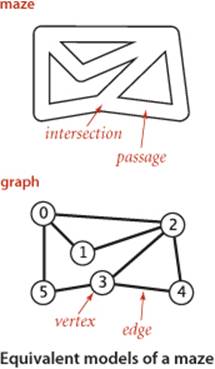

Searching in a maze
It is instructive to think about the process of searching through a graph in terms of an equivalent problem that has a long and distinguished history—finding our way through a maze that consists of passages connected by intersections. Some mazes can be handled with a simple rule, but most mazes require a more sophisticated strategy. Using the terminology maze instead of graph, passage instead of edge, and intersection instead of vertex is making mere semantic distinctions, but, for the moment, doing so will help to give us an intuitive feel for the problem. One trick for exploring a maze without getting lost that has been known since antiquity (dating back at least to the legend of Theseus and the Minotaur) is known as Tremaux exploration. To explore all passages in a maze:
• Take any unmarked passage, unrolling a string behind you.
• Mark all intersections and passages when you first visit them.
• Retrace steps (using the string) when approaching a marked intersection.
• Retrace steps when no unvisited options remain at an intersection encountered while retracing steps.
The string guarantees that you can always find a way out and the marks guarantee that you avoid visiting any passage or intersection twice. Knowing that you have explored the whole maze demands a more complicated argument that is better approached in the context of graph search. Tremaux exploration is an intuitive starting point, but it differs in subtle ways from exploring a graph, so we now move on to searching in graphs.
Warmup
The classic recursive method for searching in a connected graph (visiting all of its vertices and edges) mimics Tremaux maze exploration but is even simpler to describe. To search a graph, invoke a recursive method that visits vertices. To visit a vertex:
• Mark it as having been visited.
• Visit (recursively) all the vertices that are adjacent to it and that have not yet been marked.
Depth-first search
public class DepthFirstSearch
{
private boolean[] marked;
private int count;
public DepthFirstSearch(Graph G, int s)
{
marked = new boolean[G.V()];
dfs(G, s);
}
private void dfs(Graph G, int v)
{
marked[v] = true;
count++;
for (int w : G.adj(v))
if (!marked[w]) dfs(G, w);
}
public boolean marked(int w)
{ return marked[w]; }
public int count()
{ return count; }
}
This method is called depth-first search (DFS). An implementation of our Search API using this method is shown at right. It maintains an array of boolean values to mark all of the vertices that are connected to the source. The recursive method marks the given vertex and calls itself for any unmarked vertices on its adjacency list. If the graph is connected, every adjacency-list entry is checked.
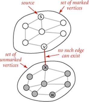
Proposition A. DFS marks all the vertices connected to a given source in time proportional to the sum of their degrees.
Proof: First, we prove that the algorithm marks all the vertices connected to the source s (and no others). Every marked vertex is connected to s, since the algorithm finds vertices only by following edges. Now, suppose that some unmarked vertex w is connected to s. Since s itself is marked, any path from s to w must have at least one edge from the set of marked vertices to the set of unmarked vertices, say v-x. But the algorithm would have discovered x after marking v, so no such edge can exist, a contradiction. The time bound follows because marking ensures that each vertex is visited once (taking time proportional to its degree to check marks).
One-way passages.
The method call–return mechanism in the program corresponds to the string in the maze: when we have processed all the edges incident to a vertex (explored all the passages leaving an intersection), we “return” (in both senses of the word). To draw a proper correspondence with Tremaux exploration of a maze, we need to imagine a maze constructed entirely of one-way passages (one in each direction). In the same way that we encounter each passage in the maze twice (once in each direction), we encounter each edge in the graph twice (once at each of its vertices). In Tremaux exploration, we either explore a passage for the first time or return along it from a marked vertex; in DFS of an undirected graph, we either do a recursive call when we encounter an edge v-w (if w is not marked) or skip the edge (if w is marked). The second time that we encounter the edge, in the opposite orientation w-v, we always ignore it, because the destination vertex v has certainly already been visited (the first time that we encountered the edge).
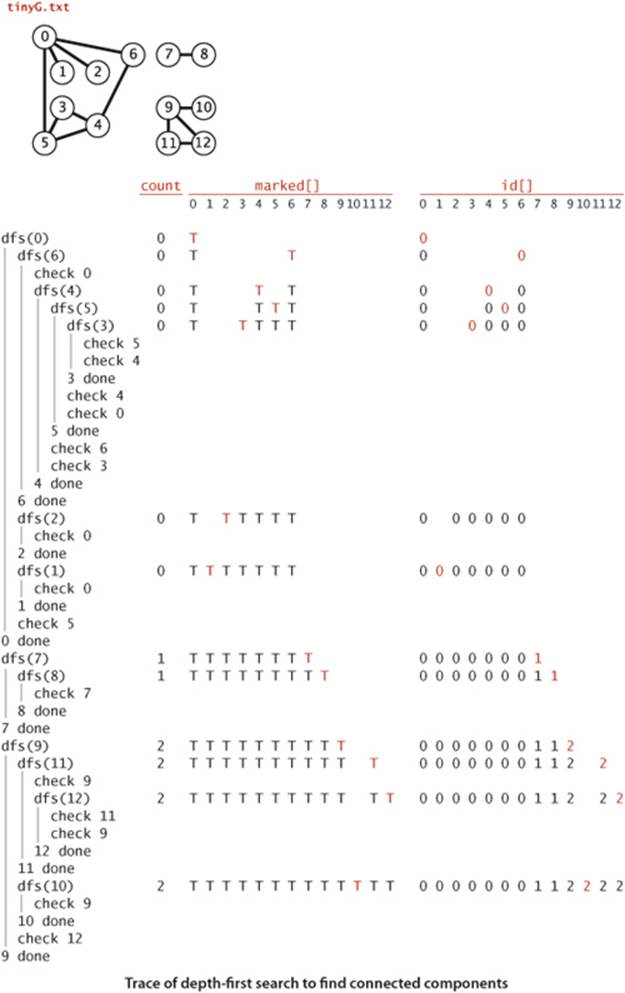
Tracing DFS
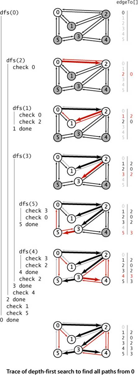
As usual, one good way to understand an algorithm is to trace its behavior on a small example. This is particularly true of depth-first search. The first thing to bear in mind when doing a trace is that the order in which edges are examined and vertices visited depends upon the representation,not just the graph or the algorithm. Since DFS only examines vertices connected to the source, we use the small connected graph depicted at left as an example for traces. In this example, vertex 2 is the first vertex visited after 0 because it happens to be first on 0’s adjacency list. The second thing to bear in mind when doing a trace is that, as mentioned above, DFS traverses each edge in the graph twice, always finding a marked vertex the second time. One effect of this observation is that tracing a DFS takes twice as long as you might think! Our example graph has only eight edges, but we need to trace the action of the algorithm on the 16 entries on the adjacency lists.
Detailed trace of depth-first search
The figure at right shows the contents of the data structures just after each vertex is marked for our small example, with source 0. The search begins when the constructor calls the recursive dfs() to mark and visit vertex 0 and proceeds as follows:
• Since 2 is first on 0’s adjacency list and is unmarked, dfs() recursively calls itself to mark and visit 2 (in effect, the system puts 0 and the current position on 0’s adjacency list on a stack).
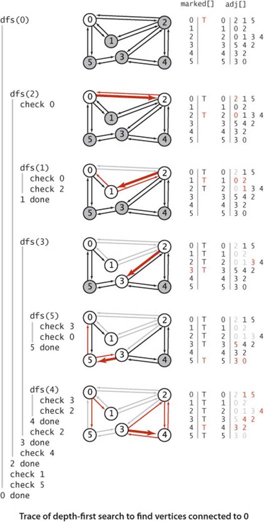
• Now, 0 is first on 2’s adjacency list and is marked, so dfs() skips it. Then, since 1 is next on 2’s adjacency list and is unmarked, dfs() recursively calls itself to mark and visit 1.
• Visiting 1 is different: since both vertices on its list (0 and 2) are already marked, no recursive calls are needed, and dfs() returns from the recursive call dfs(1). The next edge examined is 2-3 (since 3 is the vertex after 1 on 2’s adjacency list), so dfs() recursively calls itself to mark and visit 3.
• Vertex 5 is first on 3’s adjacency list and is unmarked, so dfs() recursively calls itself to mark and visit 5.
• Both vertices on 5’s list (3 and 0) are already marked, so no recursive calls are needed,
• Vertex 4 is next on 3’s adjacency list and is unmarked, so dfs() recursively calls itself to mark and visit 4, the last vertex to be marked.
• After 4 is marked, dfs() needs to check the vertices on its list, then the remaining vertices on 3’s list, then 2’s list, then 0’s list, but no more recursive calls happen because all vertices are marked.
THIS BASIC RECURSIVE SCHEME IS JUST A START—depth-first search is effective for many graph-processing tasks. For example, in this section, we consider the use of depth-first search to address a problem that we first posed in CHAPTER 1:
Connectivity. Given a graph, support queries of the form Are two given vertices connected? and How many connected components does the graph have?
This problem is easily solved within our standard graph-processing design pattern, and we will compare and contrast this solution with the union-find algorithms that we considered in SECTION 1.5.
The question “Are two given vertices connected?” is equivalent to the question “Is there a path connecting two given vertices?” and might be named the path detection problem. However, the union-find data structures that we considered in SECTION 1.5 do not address the problems of findingsuch a path. Depth-first search is the first of several approaches that we consider to solve this problem, as well:
Single-source paths. Given a graph and a source vertex s, support queries of the form Is there a path from s to a given target vertex v? If so, find such a path.
DFS is deceptively simple because it is based on a familiar concept and is so easy to implement; in fact, it is a subtle and powerful algorithm that researchers have learned to put to use to solve numerous difficult problems. These two are the first of several that we will consider.
Finding paths
The single-source paths problem is fundamental to graph processing. In accordance with our standard design pattern, we use the following API:
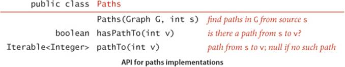
The constructor takes a source vertex s as argument and computes paths from s to each vertex connected to s. After creating a Paths object for a source s, the client can use the instance method pathTo() to iterate through the vertices on a path from s to any vertex connected to s. For the moment, we accept any path; later, we shall develop implementations that find paths having certain properties. The test client at right takes a graph from the input stream and a source from the command line and prints a path from the source to each vertex connected to it.
Test client for paths implementations
public static void main(String[] args)
{
Graph G = new Graph(new In(args[0]));
int s = Integer.parseInt(args[1]);
Paths search = new Paths(G, s);
for (int v = 0; v < G.V(); v++)
{
StdOut.print(s + " to " + v + ": ");
if (search.hasPathTo(v))
for (int x : search.pathTo(v))
if (x == s) StdOut.print(x);
else StdOut.print("-" + x);
StdOut.println();
}
}
Implementation
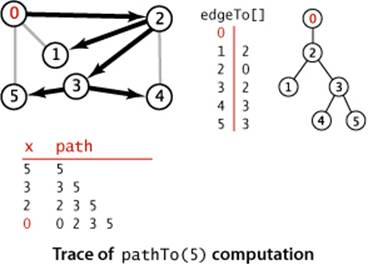
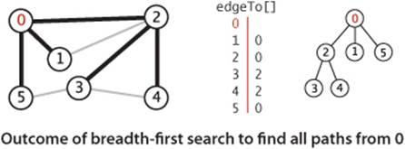
ALGORITHM 4.1 on page 536 is a DFS-based implementation of Paths that extends the DepthFirstSearch warmup on page 531 by adding as an instance variable an array edgeTo[] of int values that serves the purpose of the ball of string in Tremaux exploration: it gives a way to find a path back to s for every vertex connected to s. Instead of just keeping track of the path from the current vertex back to the start, we remember a path from each vertex to the start. To accomplish this, we remember the edge v-w that takes us to each vertex w for the first time, by setting edgeTo[w] to v. In other words,v-w is the last edge on the known path from s to w. The result of the search is a tree rooted at the source; edgeTo[] is a parent-link representation of that tree. A small example is drawn to the right of the code in ALGORITHM 4.1. To recover the path from s to any vertex v, the pathTo() method inALGORITHM 4.1 uses a variable x to travel up the tree, setting x to edgeTo[x], just as we did for union-find in SECTION 1.5, putting each vertex encountered onto a stack until reaching s. Returning the stack to the client as an Iterable enables the client to follow the path from s to v.
% java Paths tinyCG.txt 0
0 to 0: 0
0 to 1: 0-2-1
0 to 2: 0-2
0 to 3: 0-2-3
0 to 4: 0-2-3-4
0 to 5: 0-2-3-5
Algorithm 4.1 Depth-first search to find paths in a graph
public class DepthFirstPaths
{
private boolean[] marked; // Has dfs() been called for this vertex?
private int[] edgeTo; // last vertex on known path to this vertex
private final int s; // source
public DepthFirstPaths(Graph G, int s)
{
marked = new boolean[G.V()];
edgeTo = new int[G.V()];
this.s = s;
dfs(G, s);
}
private void dfs(Graph G, int v)
{
marked[v] = true;
for (int w : G.adj(v))
if (!marked[w])
{
edgeTo[w] = v;
dfs(G, w);
}
}
public boolean hasPathTo(int v)
{ return marked[v]; }
public Iterable<Integer> pathTo(int v)
{
if (!hasPathTo(v)) return null;
Stack<Integer> path = new Stack<Integer>();
for (int x = v; x != s; x = edgeTo[x])
path.push(x);
path.push(s);
return path;
}
}
This Graph client uses depth-first search to find paths to all the vertices in a graph that are connected to a given start vertex s. Code from DepthFirstSearch (page 531) is printed in gray. To save known paths to each vertex, this code maintains a vertex-indexed array edgeTo[] such that edgeTo[w] = vmeans that v-w was the edge used to access w for the first time. The edgeTo[] array is a parent-link representation of a tree rooted at s that contains all the vertices connected to s.
Detailed trace
The figure at right shows the contents of edgeTo[] just after each vertex is marked for our example, with source 0. The contents of marked[] and adj[] are the same as in the trace of DepthFirstSearch on page 533, as is the detailed description of the recursive calls and the edges checked, so these aspects of the trace are omitted. The depth-first search adds the edges 0-2, 2-1, 2-3, 3-5, and 3-4 to edgeTo[], in that order. These edges form a tree rooted at the source and provide the information needed for pathTo() to provide for the client the path from 0 to 1, 2, 3, 4, or 5, as just described.
THE CONSTRUCTOR in DepthFirstPaths differs only in a few assignment statements from the constructor in DepthFirstSearch, so PROPOSITION A on page 531 applies. In addition, we have:
Proposition A (continued). DFS allows us to provide clients with a path from a given source to any marked vertex in time proportional its length.
Proof: By induction on the number of vertices visited, it follows that the edgeTo[] array in DepthFirstPaths represents a tree rooted at the source. The pathTo() method builds the path in time proportional to its length.
Breadth-first search
The paths discovered by depth-first search depend not just on the graph, but also on the representation and the nature of the recursion. Naturally, we are often interested in solving the following problem:
Single-source shortest paths. Given a graph and a source vertex s, support queries of the form Is there a path from s to a given target vertex v? If so, find a shortest such path (one with a minimal number of edges).
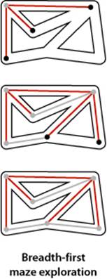
The classical method for accomplishing this task, called breadth-first search (BFS), is also the basis of numerous algorithms for processing graphs, so we consider it in detail in this section. DFS offers us little assistance in solving this problem, because the order in which it takes us through the graph has no relationship to the goal of finding shortest paths. In contrast, BFS is based on this goal. To find a shortest path from s to v, we start at s and check for v among all the vertices that we can reach by following one edge, then we check for v among all the vertices that we can reach from s by following two edges, and so forth. DFS is analogous to one person exploring a maze. BFS is analogous to a group of searchers exploring by fanning out in all directions, each unrolling his or her own ball of string. When more than one passage needs to be explored, we imagine that the searchers split up to expore all of them; when two groups of searchers meet up, they join forces (using the ball of string held by the one getting there first).
In a program, when we come to a point during a graph search where we have more than one edge to traverse, we choose one and save the others to be explored later. In DFS, we use a pushdown stack (that is managed by the system to support the recursive search method) for this purpose. Using the LIFO rule that characterizes the pushdown stack corresponds to exploring passages that are close by in a maze. We choose, of the passages yet to be explored, the one that was most recently encountered. In BFS, we want to explore the vertices in order of their distance from the source. It turns out that this order is easily arranged: use a (FIFO) queue instead of a (LIFO) stack. We choose, of the passages yet to be explored, the one that was least recently encountered.
Implementation
ALGORITHM 4.2 on page 540 is an implementation of BFS. It is based on maintaining a queue of all vertices that have been marked but whose adjacency lists have not been checked. We put the source vertex on the queue, then perform the following steps until the queue is empty:
• Take the next vertex v from the queue and mark it.
• Put onto the queue all unmarked vertices that are adjacent to v.
The bfs() method in ALGORITHM 4.2 is not recursive. Instead of the implicit stack provided by recursion, it uses an explicit queue. The product of the search, as for DFS, is an array edgeTo[], a parent-link representation of a tree rooted at s, which defines the shortest paths from s to every vertex that is connected to s. The paths can be constructed for the client using the same pathTo() implementation that we used for DFS in ALGORITHM 4.1.
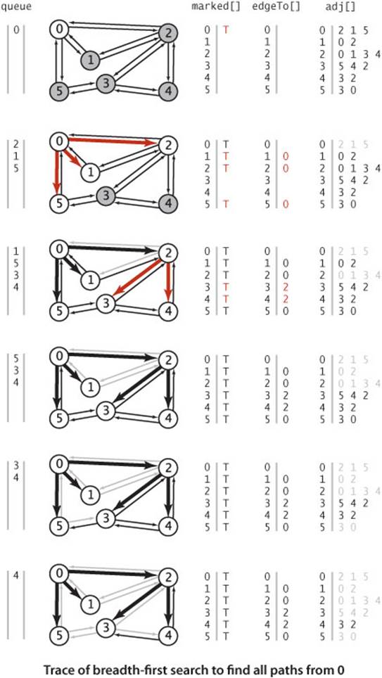
The figure at right shows the step-by-step development of BFS on our sample graph, showing the contents of the data structures at the beginning of each iteration of the loop. Vertex 0 is put on the queue, then the loop completes the search as follows:
• Removes 0 from the queue and puts its adjacent vertices 2, 1, and 5 on the queue, marking each and setting the edgeTo[] entry for each to 0.
• Removes 2 from the queue, checks its adjacent vertices 0 and 1, which are marked, and puts its adjacent vertices 3 and 4 on the queue, marking each and setting the edgeTo[] entry for each to 2.
• Removes 1 from the queue and checks its adjacent vertices 0 and 2, which are marked.
• Removes 5 from the queue and checks its adjacent vertices 3 and 0, which are marked.
• Removes 3 from the queue and checks its adjacent vertices 5, 4, and 2, which are marked.
• Removes 4 from the queue and checks its adjacent vertices 3 and 2, which are marked.
Algorithm 4.2 Breadth-first search to find paths in a graph
public class BreadthFirstPaths
{
private boolean[] marked; // Is a shortest path to this vertex known?
private int[] edgeTo; // last vertex on known path to this vertex
private final int s; // source
public BreadthFirstPaths(Graph G, int s)
{
marked = new boolean[G.V()];
edgeTo = new int[G.V()];
this.s = s;
bfs(G, s);
}
private void bfs(Graph G, int s)
{
Queue<Integer> queue = new Queue<Integer>();
marked[s] = true; // Mark the source
queue.enqueue(s); // and put it on the queue.
while (!queue.isEmpty())
{
int v = queue.dequeue(); // Remove next vertex from the queue.
for (int w : G.adj(v))
if (!marked[w]) // For every unmarked adjacent vertex,
{
edgeTo[w] = v; // save last edge on a shortest path,
marked[w] = true; // mark it because path is known,
queue.enqueue(w); // and add it to the queue.
}
}
}
public boolean hasPathTo(int v)
{ return marked[v]; }
public Iterable<Integer> pathTo(int v)
// Same as for DFS (see page 536).
}
This Graph client uses breadth-first search to find paths in a graph with the fewest number of edges from the source s given in the constructor. The bfs() method marks all vertices connected to s, so clients can use hasPathTo() to determine whether a given vertex v is connected to s and pathTo()to get a path from s to v with the property that no other such path from s to v has fewer edges.
For this example, the edgeTo[] array is complete after the second step. As with DFS, once all vertices have been marked, the rest of the computation is just checking edges to vertices that have already been marked.
Proposition B. For any vertex v reachable from s, BFS computes a shortest path from s to v (no path from s to v has fewer edges).
Proof: It is easy to prove by induction that the queue always consists of zero or more vertices of distance k from the source, followed by zero or more vertices of distance k+1 from the source, for some integer k, starting with k equal to 0. This property implies, in particular, that vertices enter and leave the queue in order of their distance from s. When a vertex v enters the queue, no shorter path to v will be found before it comes off the queue, and no path to v that is discovered after it comes off the queue can be shorter than v’s tree path length.
Proposition B (continued). BFS takes time proportional to V+E in the worst case.
Proof: As for PROPOSITION A (page 531), BFS marks all the vertices connected to s in time proportional to the sum of their degrees. If the graph is connected, this sum equals the sum of the degrees of all the vertices, or 2E. Initialzing the marked[] and edgeTo[] arrays takes time proportional to V.
Note that we can also use BFS to implement the Search API that we implemented with DFS, since the solution depends on only the ability of the search to examine every vertex and edge connected to the source.
As implied at the outset, DFS and BFS are the first of several instances that we will examine of a general approach to searching graphs. We put the source vertex on the data structure, then perform the following steps until the data structure is empty:
• Take the next vertex v from the data structure and mark it.
• Put onto the data structure all unmarked vertices that are adjacent to v.
The algorithms differ only in the rule used to take the next vertex from the data structure (least recently added for BFS, most recently added for DFS). This difference leads to completely different views of the graph, even though all the vertices and edges connected to the source are examined no matter what rule is used. Our implementations of BFS and DFS gain efficiency over the general approach by eagerly marking vertices as they are added to the data structure (BFS) and lazily adding unmarked vertices to the data structure (DFS)
% java BreadthFirstPaths tinyCG.txt 0
0 to 0: 0
0 to 1: 0-1
0 to 2: 0-2
0 to 3: 0-2-3
0 to 4: 0-2-4
0 to 5: 0-5
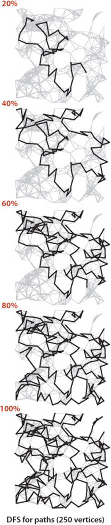
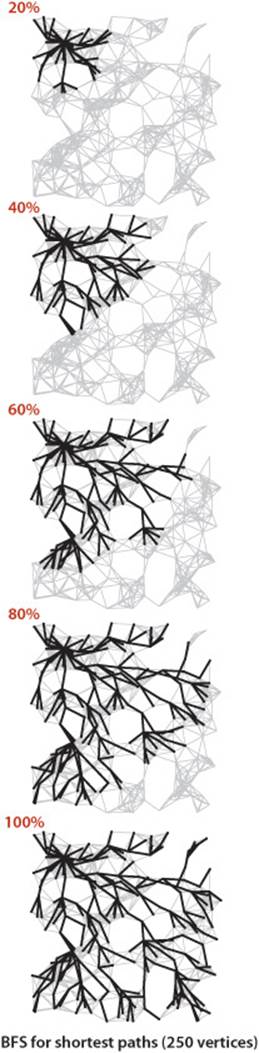
THE DIAGRAMS ON EITHER SIDE of this page, which show the progress of DFS and BFS for our sample graph mediumG.txt, make plain the differences between the paths that are discovered by the two approaches. DFS wends its way through the graph, storing on the stack the points where other paths branch off; BFS sweeps through the graph, using a queue to remember the frontier of visited places. DFS explores the graph by looking for new vertices far away from the start point, taking closer vertices only when dead ends are encountered; BFS completely covers the area close to the starting point, moving farther away only when everything nearby has been examined. DFS paths tend to be long and winding; BFS paths are short and direct. Depending upon the application, one property or the other may be desirable (or properties of paths may be immaterial). In SECTION 4.4, we will be considering other implementations of the Paths API that find paths having other specified properties.
Connected components
Our next direct application of depth-first search is to find the connected components of a graph. Recall from SECTION 1.5 (see page 216) that “is connected to” is an equivalence relation that divides the vertices into equivalence classes (the connected components). For this common graph-processing task, we define the following API:
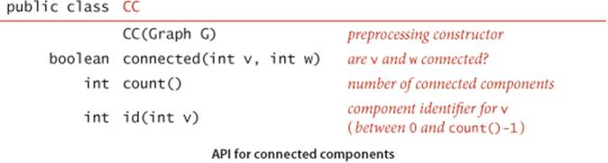
The id() method is for client use in indexing an array by component, as in the test client below, which reads a graph and then prints its number of connected components and then the vertices in each component, one component per line. To do so, it builds an array of Queue objects, then uses each vertex’s component identifier as an index into this array, to add the vertex to the appropriate Queue. This client is a model for the typical situation where we want to independently process connected components.
Test client for connected components API
public static void main(String[] args)
{
Graph G = new Graph(new In(args[0]));
CC cc = new CC(G);
int M = cc.count();
StdOut.println(M + " components");
Queue<Integer>[] components;
components = (Queue<Integer>[]) new Queue[M];
for (int i = 0; i < M; i++)
components[i] = new Queue<Integer>();
for (int v = 0; v < G.V(); v++)
components[cc.id(v)].enqueue(v);
for (int i = 0; i < M; i++)
{
for (int v: components[i])
StdOut.print(v + " ");
StdOut.println();
}
}
Implementation
The implementation CC (ALGORITHM 4.3 on the next page) uses our marked[] array to find a vertex to serve as the starting point for a depth-first search in each component. The first call to the recursive DFS is for vertex 0—it marks all vertices connected to 0. Then the for loop in the constructor looks for an unmarked vertex and calls the recursive dfs() to mark all vertices connected to that vertex. Moreover, it maintains a vertex-indexed array id[] that associates the same int value to every vertex in each component. This array makes the implementation of connected() simple, in precisely the same manner as connected() in SECTION 1.5 (just check if identifiers are equal). In this case, the identifier 0 is assigned to all the vertices in the first component processed, 1 is assigned to all the vertices in the second component processed, and so forth, so that the identifiers are all between 0and count()-1, as specified in the API. This convention enables the use of component-indexed arrays, as in the test client on page 543.
Algorithm 4.3 Depth-first search to find connected components in a graph
public class CC
{
private boolean[] marked;
private int[] id;
private int count;
public CC(Graph G)
{
marked = new boolean[G.V()];
id = new int[G.V()];
for (int s = 0; s < G.V(); s++)
if (!marked[s])
{
dfs(G, s);
count++;
}
}
private void dfs(Graph G, int v)
{
marked[v] = true;
id[v] = count;
for (int w : G.adj(v))
if (!marked[w])
dfs(G, w);
}
public boolean connected(int v, int w)
{ return id[v] == id[w]; }
public int id(int v)
{ return id[v]; }
public int count()
{ return count; }
}
% java Graph tinyG.txt
13 vertices, 13 edges
0: 6 2 1 5
1: 0
2: 0
3: 5 4
4: 5 6 3
5: 3 4 0
6: 0 4
7: 8
8: 7
9: 11 10 12
10: 9
11: 9 12
12: 11 9
% java CC tinyG.txt
3 components
0 1 2 3 4 5 6
7 8
9 10 11 12
This Graph client provides its clients with the ability to independently process a graph’s connected components. Code from DepthFirstSearch (page 531) is left in gray. The computation is based on a vertex-indexed array id[] such that id[v] is set to i if v is in the ith connected component processed. The constructor finds an unmarked vertex and calls the recursive dfs() to mark and identify all the vertices connected to it, continuing until all vertices have been marked and identified. Implementations of the instance methods connected(), id(), and count() are immediate.
Proposition C. DFS uses preprocessing time and space proportional to V+E to support constant-time connectivity queries in a graph.
Proof: Immediate from the code. Each adjacency-list entry is examined exactly once, and there are 2E such entries (two for each edge); initialzing the marked[] and id[] arrays takes time proportional to V. Instance methods examine or return one or two instance variables.
Union-find
How does the DFS-based solution for graph connectivity in CC compare with the union-find approach of CHAPTER 1? In theory, DFS is faster than union-find because it provides a constant-time guarantee, which union-find does not; in practice, this difference is negligible, and union-find is faster because it does not have to build a full representation of the graph. More important, union-find is an online algorithm (we can check whether two vertices are connected in near-constant time at any point, even while adding edges), whereas the DFS solution must first preprocess the graph. Therefore, for example, we prefer union-find when determining connectivity is our only task or when we have a large number of queries intermixed with edge insertions but may find the DFS solution more appropriate for use in a graph ADT because it makes efficient use of existing infrastructure.
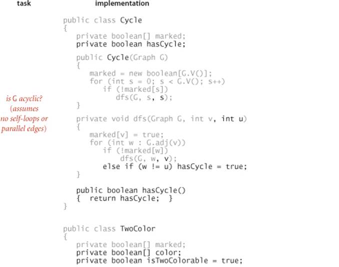
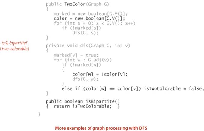
THE PROBLEMS THAT WE HAVE SOLVED with DFS are fundamental. It is a simple approach, and recursion provides us a way to reason about the computation and develop compact solutions to graph-processing problems. Two additional examples, for solving the following problems, are given in the table on the facing page.
Cycle detection. Support this query: Is a given graph acylic?
Two-colorability. Support this query: Can the vertices of a given graph be assigned one of two colors in such a way that no edge connects vertices of the same color? which is equivalent to this question: Is the graph bipartite?
As usual with DFS, the simple code masks a more sophisticated computation, so studying these examples, tracing their behavior on small sample graphs, and extending them to provide a cycle or a coloring, respectively, are worthwhile (and left for exercises).
Symbol graphs
Typical applications involve processing graphs defined in files or on web pages, using strings, not integer indices, to define and refer to vertices. To accommodate such applications, we define an input format with the following properties:
• Vertex names are strings.
• A specified delimiter separates vertex names (to allow for the possibility of spaces in names).
• Each line represents a set of edges, connecting the first vertex name on the line to each of the other vertices named on the line.
• The number of vertices V and the number of edges E are both implicitly defined.
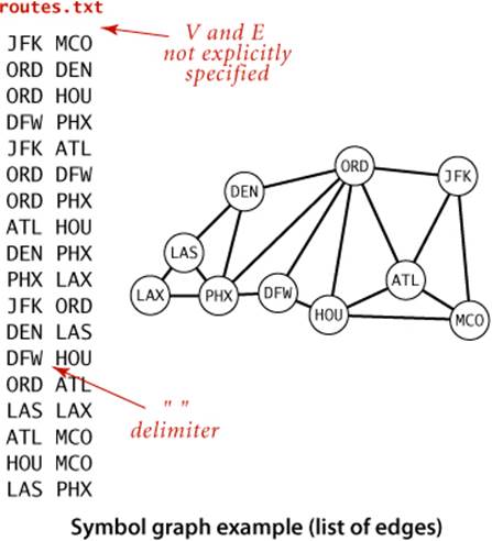
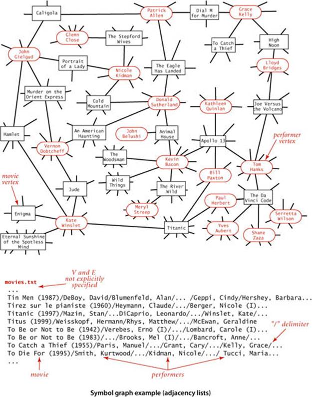
Shown below is a small example, the file routes.txt, which represents a model for a small transportation system where vertices are U.S. airport codes and edges connecting them are airline routes between the vertices. The file is simply a list of edges. Shown on the facing page is a larger example, taken from the file movies.txt, from the Internet Movie Database (IMDB), that we introduced in SECTION 3.5. Recall that this file consists of lines listing a movie name followed by a list of the performers in the movie. In the context of graph processing, we can view it as defining a graph with movies and performers as vertices and each line defining the adjacency list of edges connecting each movie to its performers. Note that the graph is a bipartite graph—there are no edges connecting performers to performers or movies to movies.
API
The following API defines a Graph client that allows us to immediately use our graph-processing routines for graphs defined by such files:
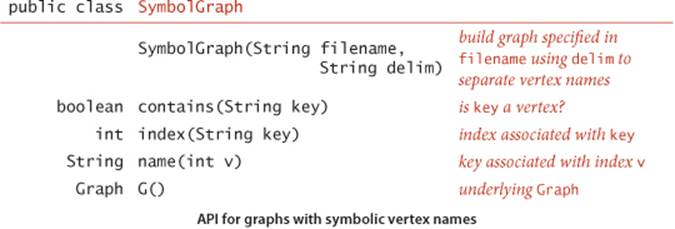
This API provides a constructor to read and build the graph and client methods name() and index() for translating vertex names between the strings on the input stream and the integer indices used by our graph-processing methods.
Test client for symbol graph API
public static void main(String[] args)
{
String filename = args[0];
String delim = args[1];
SymbolGraph sg = new SymbolGraph(filename, delim);
Graph G = sg.G();
while (StdIn.hasNextLine())
{
String source = StdIn.readLine();
for (int v : G.adj(sg.index(source)))
StdOut.println(" " + sg.name(v));
}
}
Test client
The test client at left builds a graph from the file named as the first command-line argument (using the delimiter as specified by the second command-line argument) and then takes queries from standard input. The user specifies a vertex name and gets the list of vertices adjacent to that vertex. This client immediately provides the useful inverted index functionality that we considered in SECTION 3.5. In the case of routes.txt, you can type an airport code to find the direct flights from that airport, information that is not directly available in the data file. In the case of movies.txt, you can type the name of a performer to see the list of the movies in the database in which that performer appeared, or you can type the name of a movie to see the list of performers that appear in that movie. Typing a movie name and getting its cast is not much more than regurgitating the corresponding line in the input file, but typing the name of a performer and getting the list of movies in which that performer has appeared is inverting the index. Even though the database is built around connecting movies to performers, the bipartite graph model embraces the idea that it also connects performers to movies. The bipartite graph model automatically serves as an inverted index and also provides the basis for more sophisticated processing, as we will see.
% java SymbolGraph routes.txt " "
JFK
ORD
ATL
MCO
LAX
LAS
PHX
% java SymbolGraph movies.txt "/"
Tin Men (1987)
Hershey, Barbara
Geppi, Cindy
...
Blumenfeld, Alan
DeBoy, David
Bacon, Kevin
Woodsman, The (2004)
Wild Things (1998)
...
Apollo 13 (1995)
Animal House (1978)
THIS APPROACH IS CLEARLY EFFECTIVE for any of the graph-processing methods that we consider: any client can use index() when it wants to convert a vertex name to an index for use in graph processing and name() when it wants to convert an index from graph processing into a name for use in the context of the application.
Implementation
A full SymbolGraph implementation is given on page 552. It builds three data structures:
• A symbol table st with String keys (vertex names) and int values (indices)
• An array keys[] that serves as an inverted index, giving the vertex name associated with each integer index
• A Graph G built using the indices to refer to vertices
SymbolGraph uses two passes through the data to build these data structures, primarily because the number of vertices V is needed to build the Graph. In typical real-world applications, keeping the value of V and E in the graph definition file (as in our Graph constructor at the beginning of this section) is somewhat inconvenient—with SymbolGraph, we can maintain files such as routes.txt or movies.txt by adding or deleting entries without regard to the number of different names involved.
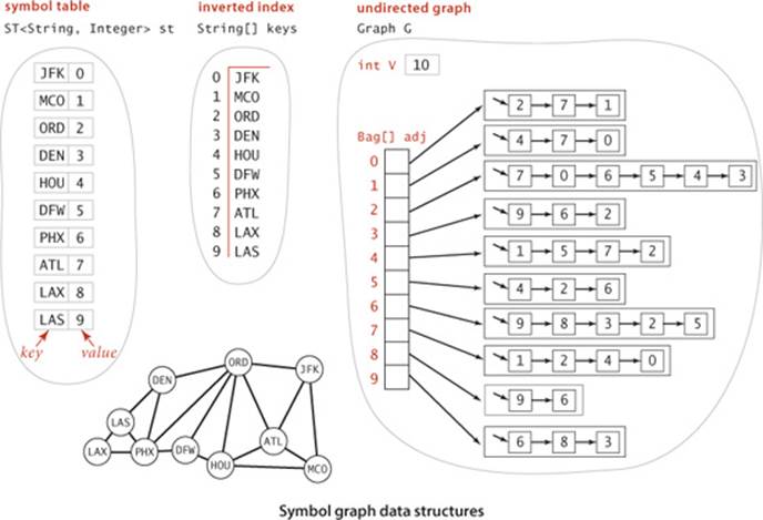
Symbol graph data type
public class SymbolGraph
{
private ST<String, Integer> st; // String -> index
private String[] keys; // index -> String
private Graph G; // the graph
public SymbolGraph(String stream, String sp)
{
st = new ST<String, Integer>();
In in = new In(stream); // First pass
while (in.hasNextLine()) // builds the index
{
String[] a = in.readLine().split(sp); // by reading strings
for (int i = 0; i < a.length; i++) // to associate each
if (!st.contains(a[i])) // distinct string
st.put(a[i], st.size()); // with an index.
}
keys = new String[st.size()]; // Inverted index
for (String name : st.keys()) // to get string keys
keys[st.get(name)] = name; // is an array.
G = new Graph(st.size());
in = new In(stream); // Second pass
while (in.hasNextLine()) // builds the graph
{
String[] a = in.readLine().split(sp); // by connecting the
int v = st.get(a[0]); // first vertex
for (int i = 1; i < a.length; i++) // on each line
G.addEdge(v, st.get(a[i])); // to all the others.
}
}
public boolean contains(String s) { return st.contains(s); }
public int index(String s) { return st.get(s); }
public String name(int v) { return keys[v]; }
public Graph G() { return G; }
}
This Graph client allows clients to define graphs with String vertex names instead of integer indices. It maintains instance variables st (a symbol table that maps names to indices), keys (an array that maps indices to names), and G (a graph, with integer vertex names). To build these data structures, it makes two passes through the graph definition (each line has a string and a list of adjacent strings, separated by the delimiter sp).
Degrees of separation
One of the classic applications of graph processing is to find the degree of separation between two individuals in a social network. To fix ideas, we discuss this application in terms of a recently popularized pastime known as the Kevin Bacon game, which uses the movie-performer graph that we just considered. Kevin Bacon is a prolific actor who has appeared in many movies. We assign every performer a Kevin Bacon number as follows: Bacon himself is 0, any performer who has been in the same cast as Bacon has a Kevin Bacon number of 1, any other performer (except Bacon) who has been in the same cast as a performer whose number is 1 has a Kevin Bacon number of 2, and so forth. For example, Meryl Streep has a Kevin Bacon number of 1 because she appeared in The River Wild with Kevin Bacon. Nicole Kidman’s number is 2: although she did not appear in any movie with Kevin Bacon, she was in Days of Thunder with Tom Cruise, and Cruise appeared in A Few Good Men with Kevin Bacon. Given the name of a performer, the simplest version of the game is to find some alternating sequence of movies and performers that leads back to Kevin Bacon. For example, a movie buff might know that Tom Hanks was in Joe Versus the Volcano with Lloyd Bridges, who was in High Noon with Grace Kelly, who was in Dial M for Murder with Patrick Allen, who was in The Eagle Has Landed with Donald Sutherland, who was inAnimal House with Kevin Bacon. But this knowledge does not suffice to establish Tom Hanks’s Bacon number (it is actually 1 because he was in Apollo 13 with Kevin Bacon). You can see that the Kevin Bacon number has to be defined by counting the movies in the shortest such sequence, so it is hard to be sure whether someone wins the game without using a computer. Of course, as illustrated in the SymbolGraph client DegreesOfSeparation on page 555, BreadthFirstPaths is the program we need to find a shortest path that establishes the Kevin Bacon number of any performer in movies.txt. This program takes a source vertex from the command line, then takes queries from standard input and prints a shortest path from the source to the query vertex. Since the graph associated with movies.txt is bipartite, all paths alternate between movies and performers, and the printed path is a “proof” that the path is valid (but not a proof that it is the shortest such path—you need to educate your friends about PROPOSITION B for that). DegreesOfSeparation also finds shortest paths in graphs that are not bipartite: for example, it finds a way to get from one airport to another in routes.txt using the fewest connections.
% java DegreesOfSeparation movies.txt "/" "Bacon, Kevin"
Kidman, Nicole
Bacon, Kevin
Woodsman, The (2004)
Grier, David Alan
Bewitched (2005)
Kidman, Nicole
Grant, Cary
Bacon, Kevin
Planes, Trains & Automobiles (1987)
Martin, Steve (I)
Dead Men Don't Wear Plaid (1982)
Grant, Cary
YOU MIGHT ENJOY USING DegreesOfSeparation to answer some entertaining questions about the movie business. For example, you can find separations between movies, not just performers. More important, the concept of separation has been widely studied in many other contexts. For example, mathematicians play this same game with the graph defined by paper co-authorship and their connection to P. Erdös, a prolific 20th-century mathematician. Similarly, everyone in New Jersey seems to have a Bruce Springsteen number of 2, because everyone in the state seems to know someone who claims to know Bruce. To play the Erdös game, you would need a database of all mathematical papers; playing the Springsteen game is a bit more challenging. On a more serious note, degrees of separation play a crucial role in the design of computer and communications networks, and in our understanding of natural networks in all fields of science.
% java DegreesOfSeparation movies.txt "/" "Animal House (1978)"
Titanic (1997)
Animal House (1978)
Allen, Karen (I)
Raiders of the Lost Ark (1981)
Taylor, Rocky (I)
Titanic (1997)
To Catch a Thief (1955)
Animal House (1978)
Vernon, John (I)
Topaz (1969)
Hitchcock, Alfred (I)
To Catch a Thief (1955)
Degrees of separation
public class DegreesOfSeparation
{
public static void main(String[] args)
{
SymbolGraph sg = new SymbolGraph(args[0], args[1]);
Graph G = sg.G();
String source = args[2];
if (!sg.contains(source))
{ StdOut.println(source + " not in database."); return; }
int s = sg.index(source);
BreadthFirstPaths bfs = new BreadthFirstPaths(G, s);
while (!StdIn.isEmpty())
{
String sink = StdIn.readLine();
if (sg.contains(sink))
{
int t = sg.index(sink);
if (bfs.hasPathTo(t))
for (int v : bfs.pathTo(t))
StdOut.println(" " + sg.name(v));
else StdOut.println("Not connected");
}
else StdOut.println("Not in database.");
}
}
}
This SymbolGraph and BreadthFirstPaths client finds shortest paths in graphs. For movies.txt, it plays the Kevin Bacon game.
% java DegreesOfSeparation routes.txt " " JFK
LAS
JFK
ORD
PHX
LAS
DFW
JFK
ORD
DFW
Summary
In this section, we have introduced several basic concepts that we will expand upon and further develop throughout the rest of this chapter:
• Graph nomenclature
• A graph representation that enables processing of huge sparse graphs
• A design pattern for graph processing, where we implement algorithms by developing clients that preprocess the graph in the constructor, building data structures that can efficiently support client queries about the graph
• Depth-first search and breadth-first search
• A class providing the capability to use symbolic vertex names
The table below summarizes the implementations of graph algorithms that we have considered. These algorithms are a proper introduction to graph processing, since variants on their code will resurface as we consider more complicated types of graphs and applications, and (consequently) more difficult graph-processing problems. The same questions involving connections and paths among vertices become much more difficult when we add direction and then weights to graph edges, but the same approaches are effective in addressing them and serve as a starting point for addressing more difficult problems.
Q&A
Q. Why not jam all of the algorithms into Graph.java?
A. Yes, we might just add query methods (and whatever private fields and methods each might need) to the basic Graph ADT definition. While this approach has some of the virtues of data abstraction that we have embraced, it also has some serious drawbacks, because the world of graph processing is significantly more expansive than the kinds of basic data structures treated in SECTION 1.3. Chief among these drawbacks are the following:
• There are many more graph-processing operations to implement than we can accurately define in a single API.
• Simple graph-processing tasks have to use the same API needed by complicated tasks.
• One method can access a field intended for use by another method, contrary to encapsulation principles that we would like to follow.
This situation is not unusual: APIs of this kind have come to be known as wide interfaces (see page 97). In a chapter filled with graph-processing algorithms, an API of this sort would be wide indeed.
Q. Does SymbolGraph really need two passes?
A. No. You could pay an extra lg V factor and support adj() directly as an ST instead of a Bag. We have an implementation along these lines in our book An Introduction to Programming in Java: An Interdisciplinary Approach.
Exercises
4.1.1 What is the maximum number of edges in a graph with V vertices and no parallel edges? What is the minimum number of edges in a graph with V vertices, none of which are isolated (have degree 0)?
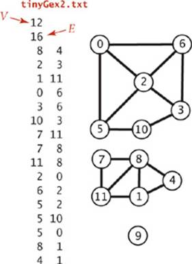
4.1.2 Draw, in the style of the figure in the text (page 524), the adjacency lists built by Graph’s input stream constructor for the file tinyGex2.txt depicted at left.
4.1.3 Create a copy constructor for Graph that takes as input a graph G and creates and initializes a new copy of the graph. Any changes a client makes to G should not affect the newly created graph.
4.1.4 Add a method hasEdge() to Graph which takes two int arguments v and w and returns true if the graph has an edge v-w, false otherwise.
4.1.5 Modify Graph to disallow parallel edges and self-loops.
4.1.6 Consider the four-vertex graph with edges 0-1, 1-2, 2-3, and 3-0. Draw an array of adjacency-lists that could not have been built calling addEdge() for these edges no matter what order.
4.1.7 Develop a test client for Graph that reads a graph from the input stream named as command-line argument and then prints it, relying on toString().
4.1.8 Develop an implementation for the Search API on page 528 that uses UF, as described in the text.
4.1.9 Show, in the style of the figure on page 533, a detailed trace of the call dfs(0) for the graph built by Graph’s input stream constructor for the file tinyGex2.txt (see EXERCISE 4.1.2). Also, draw the tree represented by edgeTo[].
4.1.10 Prove that every connected graph has a vertex whose removal (including all incident edges) will not disconnect the graph, and write a DFS method that finds such a vertex. Hint: Consider a vertex whose adjacent vertices are all marked.
4.1.11 Draw the tree represented by edgeTo[] after the call bfs(G, 0) in ALGORITHM 4.2 for the graph built by Graph’s input stream constructor for the file tinyGex2.txt (see EXERCISE 4.1.2).
4.1.12 What does the BFS tree tell us about the distance from v to w when neither is at the root?
4.1.13 Add a distTo() method to the BreadthFirstPaths API and implementation, which returns the number of edges on the shortest path from the source to a given vertex. A distTo() query should run in constant time.
4.1.14 Suppose you use a stack instead of a queue when running breadth-first search. Does it still compute shortest paths?
4.1.15 Modify the input stream constructor for Graph to also allow adjacency lists from standard input (in a manner similar to SymbolGraph), as in the example tinyGadj.txt shown at right. After the number of vertices and edges, each line contains a vertex and its list of adjacent vertices.
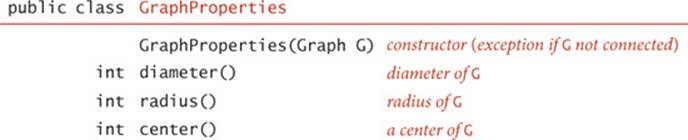
4.1.16 The eccentricity of a vertex v is the length of the shortest path from that vertex to the furthest vertex from v. The diameter of a graph is the maximum eccentricity of any vertex. The radius of a graph is the smallest eccentricity of any vertex. A center is a vertex whose eccentricity is the radius. Implement the following API:
4.1.17 The Wiener index of a graph is the sum of the lengths of the shortest paths between all pairs of vertices. Mathematical chemists use this quantity to analyze molecular graphs, where vertices correspond to atoms and edges correspond to chemical bonds. Add a method wiener() toGraphProperties that returns the Wiener index of a graph.
4.1.18 The girth of a graph is the length of its shortest cycle. If a graph is acyclic, then its girth is infinite. Add a method girth() to GraphProperties that returns the girth of the graph. Hint: Run BFS from each vertex. The shortest cycle containing s is an edge between s and some vertex vconcatenated with a shortest path between s and v (that does’t use the edge s-v)
4.1.19 Show, in the style of the figure on page 545, a detailed trace of CC for finding the connected components in the graph built by Graph’s input stream constructor for the file tinyGex2.txt (see EXERCISE 4.1.2).
4.1.20 Show, in the style of the figures in this section, a detailed trace of Cycle for finding a cycle in the graph built by Graph’s input stream constructor for the file tinyGex2.txt (see EXERCISE 4.1.2). What is the order of growth of the running time of the Cycle constructor, in the worst case?
4.1.21 Show, in the style of the figures in this section, a detailed trace of TwoColor for finding a two-coloring of the graph built by Graph’s input stream constructor for the file tinyGex2.txt (see EXERCISE 4.1.2). What is the order of growth of the running time of the TwoColor constructor, in the worst case?
4.1.22 Run SymbolGraph with movies.txt to find the Kevin Bacon number of this year’s Oscar nominees.
4.1.23 Write a program BaconHistogram that prints a histogram of Kevin Bacon numbers, indicating how many performers from movies.txt have a Bacon number of 0, 1, 2, 3, .... Include a category for those who have an infinite number (not connected to Kevin Bacon).
4.1.24 Compute the number of connected components in movies.txt, the size of the largest component, and the number of components of size less than 10. Find the eccentricity, diameter, radius, a center, and the girth of the largest component in the graph. Does it contain Kevin Bacon?
4.1.25 Modify DegreesOfSeparation to take an int value y as a command-line argument and ignore movies that are more than y years old.
4.1.26 Write a SymbolGraph client like DegreesOfSeparation that uses depth-first search instead of breadth-first search to find paths connecting two performers, producing output like that shown on the facing page.
4.1.27 Determine the amount of memory used by Graph to represent a graph with V vertices and E edges, using the memory-cost model of SECTION 1.4.
4.1.28 Two graphs are isomorphic if there is a way to rename the vertices of one to make it identical to the other. Draw all the nonisomorphic graphs with two, three, four, and five vertices.
4.1.29 Modify Cycle so that it works even if the graph contains self-loops and parallel edges.
% java DegreesOfSeparationDFS movies.txt "/" "Bacon, Kevin"
Kidman, Nicole
Bacon, Kevin
Woodsman, The (2004)
Sedgwick, Kyra
Something to Talk About (1995)
Gillan, Lisa Roberts
Runaway Bride (1999)
Schertler, Jean
... [1782 movies ] (!)
Eskelson, Dana
Interpreter, The (2005)
Silver, Tracey (II)
Copycat (1995)
Chua, Jeni
Metro (1997)
Ejogo, Carmen
Avengers, The (1998)
Atkins, Eileen
Hours, The (2002)
Kidman, Nicole
Creative Problems
4.1.30 Eulerian and Hamiltonian cycles. Consider the graphs defined by the following four sets of edges:
0-1 0-2 0-3 1-3 1-4 2-5 2-9 3-6 4-7 4-8 5-8 5-9 6-7 6-9 7-8
0-1 0-2 0-3 1-3 0-3 2-5 5-6 3-6 4-7 4-8 5-8 5-9 6-7 6-9 8-8
0-1 1-2 1-3 0-3 0-4 2-5 2-9 3-6 4-7 4-8 5-8 5-9 6-7 6-9 7-8
4-1 7-9 6-2 7-3 5-0 0-2 0-8 1-6 3-9 6-3 2-8 1-5 9-8 4-5 4-7
Which of these graphs have Euler cycles (cycles that visit each edge exactly once)? Which of them have Hamilton cycles (cycles that visit each vertex exactly once)? Develop a linear-time DFS-based algorithm to determine whether a graph has an Euler cycle (and if so find one).
4.1.31 Graph enumeration. How many different undirected graphs are there with V vertices and E edges (and no parallel edges)?
4.1.32 Parallel edge detection. Devise a linear-time algorithm to count the parallel edges in a graph.
4.1.33 Odd cycles. Prove that a graph is two-colorable (bipartite) if and only if it contains no odd-length cycle.
4.1.34 Symbol graph. Implement a one-pass SymbolGraph (it need not be a Graph client). Your implementation may pay an extra log V factor for graph operations, for symbol-table lookups.
4.1.35 Biconnectedness. A graph is biconnected if every pair of vertices is connected by two disjoint paths. An articulation point in a connected graph is a vertex that would disconnect the graph if it (and its incident edges) were removed. Prove that any graph with no articulation points is biconnected. Hint: Given a pair of vertices s and t and a path connecting them, use the fact that none of the vertices on the path are articulation points to construct two disjoint paths connecting s and t.
4.1.36 Two-edge connectivity. A bridge in a graph is an edge that, if removed, would increase the number of connected components. A graph that has no bridges is said to be two-edge connected. Develop a linear-time DFS-based algorithm for determining whether a given graph is edge connected.
4.1.37 Euclidean graphs. Design and implement an API EuclideanGraph for graphs whose vertices are points in the plane that include coordinates. Include a method show() that uses StdDraw to draw the graph.
4.1.38 Image processing. Implement the flood fill operation on the implicit graph defined by connecting adjacent points that have the same color in an image. Hint: Avoid an explicit stack.
Experiments
4.1.39 Random graphs. Write a program ErdosRenyiGraph that takes integer values V and E from the command line and builds a graph by generating E random pairs of integers between 0 and V−1. Note: This generator produces self-loops and parallel edges.
4.1.40 Random simple graphs. Write a program RandomSimpleGraph that takes integer values V and E from the command line and produces, with equal likelihood, each of the possible simple graphs with V vertices and E edges.
4.1.41 Random sparse graphs. Write a program RandomSparseGraph to generate random sparse graphs for a well-chosen set of values of V and E such that you can use it to run meaningful empirical tests on graphs drawn from the Erdös-Renyi model.
4.1.42 Random Euclidean graphs. Write a EuclideanGraph client (see EXERCISE 4.1.37) RandomEuclideanGraph that produces random graphs by generating V random points in the unit (x and y-coordinates between 0 and 1), then connecting each point with all points that are within a circle of radius dcentered at that point. Note: The graph will almost certainly be connected if d is larger than the threshold value ![]() and almost certainly disconnected if d is smaller than that value.
and almost certainly disconnected if d is smaller than that value.
4.1.43 Random grid graphs. Write a EuclideanGraph client RandomGridGraph that generates random graphs by connecting vertices arranged in a ![]() -by-
-by-![]() grid to their neighbors (see EXERCISE 1.5.18). Augment your program to add R extra random edges. For large R, shrink the grid so that the total number of edges remains about 2V. Add an option such that an extra edge goes from a vertex s to a vertex t with probability inversely proportional to the Euclidean distance between s and t.
grid to their neighbors (see EXERCISE 1.5.18). Augment your program to add R extra random edges. For large R, shrink the grid so that the total number of edges remains about 2V. Add an option such that an extra edge goes from a vertex s to a vertex t with probability inversely proportional to the Euclidean distance between s and t.
4.1.44 Real-world graphs. Find a large weighted graph on the web—perhaps a map with distances, telephone connections with costs, or an airline rate schedule. Write a program RandomRealGraph that builds a graph by choosing V vertices at random and E edges at random from the subgraph induced by those vertices.
4.1.45 Random interval graphs. Consider a collection of V intervals on the real line (pairs of real numbers). Such a collection defines an interval graph with one vertex corresponding to each interval, with edges between vertices if the corresponding intervals intersect (have any points in common). Write a program that generates V random intervals in the unit interval, all of length d, then builds the corresponding interval graph. Hint: Use a BST.
4.1.46 Random transportation graphs. One way to define a transportation system is with a set of sequences of vertices, each sequence defining a path connecting the vertices. For example, the sequence 0-9-3-2 defines the edges 0-9, 9-3, and 3-2. Write a EuclideanGraph client RandomTransportation that builds a graph from an input file consisting of one sequence per line, using symbolic names. Develop input suitable to allow you to use your program to build a graph corresponding to the Paris Métro system.
Testing all algorithms and studying all parameters against all graph models is unrealistic. For each problem listed below, write a client that addresses the problem for any given input graph, then choose among the generators above to run experiments for that graph model. Use your judgment in selecting experiments, perhaps in response to results of previous experiments. Write a narrative explaining your results and any conclusions that might be drawn.
4.1.47 Path lengths in DFS. Run experiments to determine empirically the probability that DepthFirstPaths finds a path between two randomly chosen vertices and to calculate the average length of the paths found, for various graph models.
4.1.48 Path lengths in BFS. Run experiments to determine empirically the probability that BreadthFirstPaths finds a path between two randomly chosen vertices and to calculate the average length of the paths found, for various graph models.
4.1.49 Connected components. Run experiments to determine empirically the distribution of the number of components in random graphs of various types, by generating large numbers of graphs and drawing a histogram.
4.1.50 Two-colorable. Most graphs are not two-colorable, and DFS tends to discover that fact quickly. Run empirical tests to study the number of edges examined by TwoColor, for various graph models.
All materials on the site are licensed Creative Commons Attribution-Sharealike 3.0 Unported CC BY-SA 3.0 & GNU Free Documentation License (GFDL)
If you are the copyright holder of any material contained on our site and intend to remove it, please contact our site administrator for approval.
© 2016-2026 All site design rights belong to S.Y.A.