Algorithms (2014)
Four. Graphs
4.3 Minimum Spanning Trees
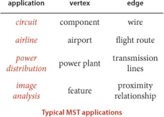
AN edge-weighted graph is a graph model where we associate weights or costs with each edge. Such graphs are natural models for many applications. In an airline map where edges represent flight routes, these weights might represent distances or fares. In an electric circuit where edges represent wires, the weights might represent the length of the wire, its cost, or the time that it takes a signal to propagate through it. Minimizing cost is naturally of interest in such situations. In this section, we consider undirected edge-weighted graph models and examine algorithms for one such problem:
Minimum spanning tree. Given an undirected edge-weighted graph, find an MST.
Definition. Recall that a spanning tree of a graph is a connected subgraph with no cycles that includes all the vertices. A minimum spanning tree (MST) of an edge-weighted graph is a spanning tree whose weight (the sum of the weights of its edges) is no larger than the weight of any other spanning tree.
In this section, we examine two classical algorithms for computing MSTs: Prim’s algorithm and Kruskal’s algorithm. These algorithms are easy to understand and not difficult to implement. They are among the oldest and most well-known algorithms in this book, and they also take good advantage of modern data structures. Since MSTs have numerous important applications, algorithms to solve the problem have been studied at least since the 1920s, at first in the context of power distribution networks, later in the context of telephone networks. MST algorithms are now important in the design of many types of networks (communication, electrical, hydraulic, computer, road, rail, air, and many others) and also in the study of biological, chemical, and physical networks that are found in nature.
Assumptions
Various anomalous situations, which are generally easy to handle, can arise when computing minimum spanning trees. To streamline the presentation, we adopt the following conventions:
• The graph is connected. The spanning-tree condition in our definition implies that the graph must be connected for an MST to exist. Another way to pose the problem, recalling basic properties of trees from SECTION 4.1, is to find a minimal-weight set of V−1 edges that connect the graph. If a graph is not connected, we can adapt our algorithms to compute the MSTs of each of its connected components, collectively known as a minimum spanning forest (see EXERCISE 4.3.22).
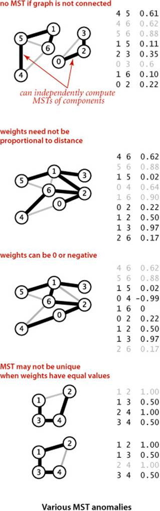
• The edge weights are not necessarily distances. Geometric intuition is sometimes beneficial in understanding algorithms, so we use examples where vertices are points in the plane and weights are distances, such as the graph on the facing page. But it is important to remember that the weights might represent time or cost or an entirely different variable and do not need to be proportional to a distance at all.
• The edge weights may be zero or negative. If the edge weights are all positive, it suffices to define an MST as a subgraph with minimal total weight that connects all the vertices, as such a subgraph must form a spanning tree. The spanning-tree condition in the definition is included so that it applies to graphs that may have zero or negative edge weights.
• The edge weights are all different. If edges can have equal weights, the minimum spanning tree may not be unique (see EXERCISE 4.3.2). The possibility of multiple MSTs complicates the correctness proofs of some of our algorithms, so we rule out that possibility in the presentation. It turns out that this assumption is not restrictive because our algorithms work without modification in the presence of equal weights.
In summary, we assume throughout the presentation that our job is to find the MST of a connected edge-weighted graph with arbitrary (but distinct) weights.
Underlying principles
To begin, we recall from SECTION 4.1 two of the defining properties of a tree:
• Adding an edge that connects two vertices in a tree creates a unique cycle.
• Removing an edge from a tree breaks it into two separate subtrees.

These properties are the basis for proving a fundamental property of MSTs that leads to the MST algorithms that we consider in this section.
Cut property
This property, which we refer to as the cut property, has to do with identifying edges that must be in the MST of a given edge-weighted graph, by dividing vertices into two sets and examining edges that cross the division.
Definition. A cut of a graph is a partition of its vertices into two nonempty disjoint sets. A crossing edge of a cut is an edge that connects a vertex in one set with a vertex in the other.
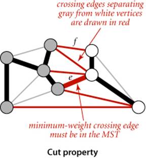
Typically, we specify a cut by specifying a set of vertices, leaving implicit the assumption that the cut comprises the given vertex set and its complement, so that a crossing edge is an edge from a vertex in the set to a vertex not in the set. In figures, we draw vertices on one side of the cut in gray and vertices on the other side in white.
Proposition J. (Cut property) Given any cut in an edge-weighted graph, the crossing edge of minimum weight is in the MST of the graph.
Proof: Let e be the crossing edge of minimum weight and let T be the MST. The proof is by contradiction: Suppose that T does not contain e. Now consider the graph formed by adding e to T. This graph has a cycle that contains e, and that cycle must contain at least one other crossing edge—say, f, which has higher weight than e (since e is minimal and all edge weights are different). We can get a spanning tree of strictly lower weight by deleting f and adding e, contradicting the assumed minimality of T.
Under our assumption that edge weights are distinct, every connected graph has a unique MST (see EXERCISE 4.3.3); and the cut property says that the lightest crossing edge for every cut must be in the MST.
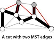
The figure to the left of PROPOSITION J illustrates the cut property. Note that there is no requirement that the minimal edge be the only MST edge connecting the two sets; indeed, for typical cuts there are several MST edges that connect a vertex in one set with a vertex in the other, as illustrated in the figure above.
Greedy algorithm
The cut property is the basis for the algorithms that we consider for the MST problem. Specifically, they are special cases of a general paradigm known as the greedy algorithm: apply the cut property to accept an edge as an MST edge, continuing until finding all of the MST edges. Our algorithms differ in their approaches to maintaining cuts and identifying the crossing edge of minimum weight, but are special cases of the following:
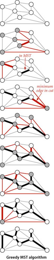
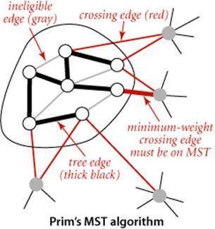
Proposition K. (Greedy MST algorithm) The following method colors black all edges in the the MST of any connected edge-weighted graph with V vertices: starting with all edges colored gray, find a cut with no black edges, color its minimum-weight edge black, and continue until V−1 edges have been colored black.
Proof: For simplicity, we assume in the discussion that the edge weights are all different, though the proposition is still true when that is not the case (see EXERCISE 4.3.5). By the cut property, any edge that is colored black is in the MST. If fewer than V−1 edges are black, a cut with no black edges exists (recall that we assume the graph to be connected). Once V−1 edges are black, the black edges form a spanning tree.
The diagram at right is a typical trace of the greedy algorithm. Each drawing depicts a cut and identifies the minimum-weight edge in the cut (thick red) that is added to the MST by the algorithm.
Edge-weighted graph data type
How should we represent edge-weighted graphs? Perhaps the simplest way to proceed is to extend the basic graph representations from SECTION 4.1: in the adjacency-matrix representation, the matrix can contain edge weights rather than boolean values; in the adjacency-lists representation, we can define a node that contains both a vertex and a weight field to put in the adjacency lists. (As usual, we focus on sparse graphs and leave the adjacency-matrix representation for exercises.) This classic approach is appealing, but we will use a different method that is not much more complicated, will make our programs useful in more general settings, and needs a slightly more general API, which allows us to process Edge objects:
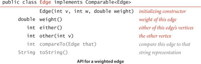
The either() and other() methods for accessing the edge’s vertices may be a bit puzzling at first—the need for them will become plain when we examine client code. You can find an implementation of Edge on page 610. It is the basis for this EdgeWeightedGraph API, which refers to Edge objects in a natural manner:
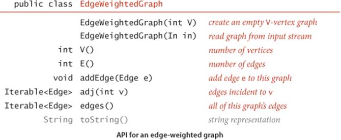
This API is very similar to the API for Graph (page 522). The two important differences are that it is based on Edge and that it adds the edges() method at right, which provides clients with the ability to iterate through all the graph’s edges (ignoring any self-loops). The rest of the implementation ofEdgeWeightedGraph on page 611 is quite similar to the unweighted undirected graph implementation of SECTION 4.1, but instead of the adjacency lists of integers used in Graph, it uses adjacency lists of Edge objects.
Gathering all the edges in an edge-weighted graph
public Iterable<Edge> edges()
{
Bag<Edge> b = new Bag<Edge>();
for (int v = 0; v < V; v++)
for (Edge e : adj[v])
if (e.other(v) > v) b.add(e);
return b;
}
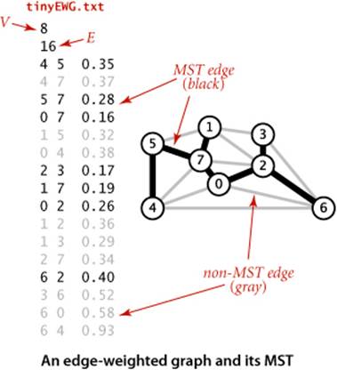
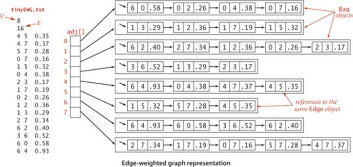
The figure at the bottom of this page shows the edge-weighted graph representation that EdgeWeightedGraph builds from the sample file tinyEWG.txt, showing the contents of each Bag as a linked list to reflect the standard implementation of SECTION 1.3. To reduce clutter in the figure, we show each Edgeas a pair of int values and a double value. The actual data structure is a linked list of links to objects containing those values. In particular, although there are two references to each Edge (one in the list for each vertex), there is only one Edge object corresponding to each graph edge. In the figure, the edges appear in each list in reverse order of the order they are processed, because of the stack-like nature of the standard linked-list implementation. As in Graph, by using a Bag we are making clear that our client code makes no assumptions about the order of objects in the lists.
Weighted edge data type
public class Edge implements Comparable<Edge>
{
private final int v; // one vertex
private final int w; // the other vertex
private final double weight; // edge weight
public Edge(int v, int w, double weight)
{
this.v = v;
this.w = w;
this.weight = weight;
}
public double weight()
{ return weight; }
public int either()
{ return v; }
public int other(int vertex)
{
if (vertex == v) return w;
else if (vertex == w) return v;
else throw new RuntimeException("Inconsistent edge");
}
public int compareTo(Edge that)
{
if (this.weight() < that.weight()) return -1;
else if (this.weight() > that.weight()) return +1;
else return 0;
}
public String toString()
{ return String.format("%d-%d %.5f", v, w, weight); }
}
This data type provides the methods either() and other() so that a client can use other(v) to find the other vertex when it knows v. When neither vertex is known, a client can use the idiomatic code int v = e.either(), w = e.other(v); to access an Edge e’s two vertices.
Edge-weighted graph data type
public class EdgeWeightedGraph
{
private final int V; // number of vertices
private int E; // number of edges
private Bag<Edge>[] adj; // adjacency lists
public EdgeWeightedGraph(int V)
{
this.V = V;
this.E = 0;
adj = (Bag<Edge>[]) new Bag[V];
for (int v = 0; v < V; v++)
adj[v] = new Bag<Edge>();
}
public EdgeWeightedGraph(In in)
// See Exercise 4.3.9.
public int V() { return V; }
public int E() { return E; }
public void addEdge(Edge e)
{
int v = e.either(), w = e.other(v);
adj[v].add(e);
adj[w].add(e);
E++;
}
public Iterable<Edge> adj(int v)
{ return adj[v]; }
public Iterable<Edge> edges()
// See page 609.
}
This implementation maintains a vertex-indexed array of lists of edges. As with Graph (see page 526), every edge appears twice: if an edge connects v and w, it appears both in v’s list and in w’s list. The edges() method puts all the edges in a Bag (see page 609). The toString() implementation is left as an exercise.
Comparing edges by weight
The API specifies that the Edge class must implement the Comparable interface and include a compareTo() implementation. The natural ordering for edges in an edge-weighted graph is by weight. Accordingly, the implementation of compareTo() is straightforward.
Parallel edges
As with our undirected-graph implementations, we allow parallel edges. Alternatively, we could develop a more complicated implementation of EdgeWeightedGraph that disallows them, perhaps keeping the minimum-weight edge from a set of parallel edges.
Self-loops
We allow self-loops. However, our edges() implementation in EdgeWeightedGraph does not include self-loops even though they might be present in the input or in the data structure. This omission has no effect on our MST algorithms because no MST contains a self-loop. When working with an application where self-loops are significant, you may need to modify our code as appropriate for the application.
OUR CHOICE TO USE explicit Edge objects leads to clear and compact client code, as you will see. It carries a small price: each adjacency-list node has a reference to an Edge object, with redundant information (all the nodes on v’s adjacency list have a v). We also pay object overhead cost. Although we have only one copy of each Edge, we do have two references to each Edge object. An alternative and widely used approach is to keep two list nodes corresponding to each edge, just as in Graph, each with a vertex and the edge weight in each list node. This alternative also carries a price—two nodes, including two copies of the weight for each edge.
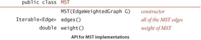
MST API and test client
As usual, for graph processing, we define an API where the constructor takes an edge-weighted graph as argument and supports client query methods that return the MST and its weight. How should we represent the MST itself? The MST of a graph G is a subgraph of G that is also a tree, so we have numerous options. Chief among them are
• A list of edges
• An edge-weighted graph
• A vertex-indexed array with parent links
To give clients and our implementations as much flexibility as possible in choosing among these alternatives for various applications, we adopt the following API:
Test client
As usual, we create sample graphs and develop a test client for use in testing our implementations. A sample client is shown below. It reads edges from the input stream, builds an edge-weighted graph, computes the MST of that graph, prints the MST edges, and prints the total weight of the MST.
MST test client
public static void main(String[] args)
{
In in = new In(args[0]);
EdgeWeightedGraph G;
G = new EdgeWeightedGraph(in);
MST mst = new MST(G);
for (Edge e : mst.edges())
StdOut.println(e);
StdOut.printf("%.5f\n", mst.weight());
}
Test data
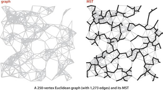
You can find the file tinyEWG.txt on the booksite, which defines the small sample graph on page 604 that we use for detailed traces of MST algorithms. You can also find on the booksite the file mediumEWG.txt, which defines the weighted graph with 250 vertices that is drawn on bottom of the the facing page. It is an example of a Euclidean graph, whose vertices are points in the plane and whose edges are lines connecting them with weights equal to their Euclidean distances. Such graphs are useful for gaining insight into the behavior of MST algorithms, and they also model many of the typical practical problems we have mentioned, such as road maps or electric circuits. You can also find on the booksite a larger example largeEWG.txt that defines a Euclidean graph with 1 million vertices. Our goal is to be able to find the MST of such a graph in a reasonable amount of time.
% more tinyEWG.txt
8 16
4 5 .35
4 7 .37
5 7 .28
0 7 .16
1 5 .32
0 4 .38
2 3 .17
1 7 .19
0 2 .26
1 2 .36
1 3 .29
2 7 .34
6 2 .40
3 6 .52
6 0 .58
6 4 .93
% java MST tinyEWG.txt
0-7 0.16000
2-3 0.17000
1-7 0.19000
0-2 0.26000
5-7 0.28000
4-5 0.35000
6-2 0.40000
1.81000
% more mediumEWG.txt
250 1273
244 246 0.11712
239 240 0.10616
238 245 0.06142
235 238 0.07048
233 240 0.07634
232 248 0.10223
231 248 0.10699
229 249 0.10098
228 241 0.01473
226 231 0.07638
... [1263 more edges ]
% java MST mediumEWG.txt
0 225 0.02383
49 225 0.03314
44 49 0.02107
44 204 0.01774
49 97 0.03121
202 204 0.04207
176 202 0.04299
176 191 0.02089
68 176 0.04396
58 68 0.04795
... [239 more edges ]
10.46351
Prim’s algorithm
Our first MST method, known as Prim’s algorithm, is to attach a new edge to a single growing tree at each step. Start with any vertex as a single-vertex tree; then add V−1 edges to it, always taking next (coloring black) the minimum-weight edge that connects a vertex on the tree to a vertex not yet on the tree (a crossing edge for the cut defined by tree vertices).
Proposition L. Prim’s algorithm computes the MST of any connected edge-weighted graph.
Proof: Immediate from PROPOSITION K. The growing tree defines a cut with no black edges; the algorithm takes the crossing edge of minimal weight, so it is successively coloring edges black in accordance with the greedy algorithm.
The one-sentence description of Prim’s algorithm just given leaves unanswered a key question: How do we (efficiently) find the crossing edge of minimal weight? Several methods have been proposed—we will discuss some of them after we have developed a full solution based on a particularly simple approach.
Data structures
We implement Prim’s algorithm with the aid of a few simple and familiar data structures. In particular, we represent the vertices on the tree, the edges on the tree, and the crossing edges, as follows:
• Vertices on the tree: We use a vertex-indexed boolean array marked[], where marked[v] is true if v is on the tree.
• Edges in the tree: We use one of two data structures: either a queue mst to collect edges in the MST edges or a vertex-indexed array edgeTo[] of Edge objects, where edgeTo[v] is the Edge that connects v to the tree.
• Crossing edges: We use a MinPQ<Edge> priority queue that compares edges by weight (see page 610).
These data structures allow us to directly answer the basic question “Which is the minimal-weight crossing edge?”
Maintaining the set of crossing edges
Each time that we add an edge to the tree, we also add a vertex to the tree. To maintain the set of crossing edges, we need to add to the priority queue all edges from that vertex to any non-tree vertex (using marked[] to identify such edges). But we must do more: any edge connecting the vertex just added to a tree vertex that is already on the priority queue now becomes ineligible (it is no longer a crossing edge because it connects two tree vertices). An eager implementation of Prim’s algorithm would remove such edges from the priority queue; we first consider a simpler lazyimplementation of the algorithm where we leave such edges on the priority queue, deferring the eligibility test to when we remove them.
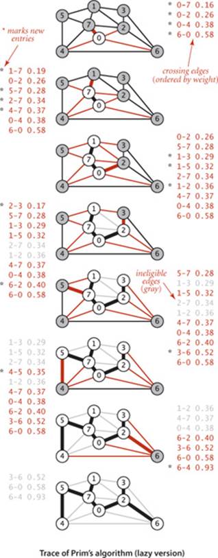
The figure at right is a trace for our small sample graph tinyEWG.txt. Each drawing depicts the graph and the priority queue just after a vertex is visited (added to the tree and the edges in its adjacency list processed). The contents of the priority queue are shown in order on the side, with new edges marked with asterisks. The algorithm builds the MST as follows:
• Adds 0 to the MST and all edges in its adjacency list to the priority queue.
• Adds 7 and 0-7 to the MST and all edges in its adjacency list to the priority queue.
• Adds 1 and 1-7 to the MST and all edges in its adjacency list to the priority queue.
• Adds 2 and 0-2 to the MST and edges 2-3 and 6-2 to the priority queue. Edges 2-7 and 1-2 become ineligible.
• Adds 3 and 2-3 to the MST and edge 3-6 to the priority queue. Edge 1-3 becomes ineligible.
• Adds 5 and 5-7 to the MST and edge 4-5 to the priority queue. Edge 1-5 becomes ineligible.
• Removes ineligible edges 1-3, 1-5, and 2-7 from the priority queue.
• Adds 4 and 4-5 to the MST and edge 6-4 to the priority queue. Edges 4-7 and 0-4 become ineligible.
• Removes ineligible edges 1-2, 4-7, and 0-4 from the priority queue.
• Adds 6 and 6-2 to the MST. The other edges incident to 6 become ineligible.
After having added V vertices (and V−1 edges), the MST is complete. The remaining edges on the priority queue are ineligible, so we need not examine them again.
Implementation
With these preparations, implementing Prim’s algorithm is straightforward, as shown in the implementation LazyPrimMST on the facing page. As with our depth-first search and breadth-first search implementations in the previous two sections, it computes the MST in the constructor so that client methods can learn properties of the MST with query methods. We use a private method visit() that puts a vertex on the tree, by marking it as visited and then putting all of its incident edges that are not ineligible onto the priority queue, thus ensuring that the priority queue contains the crossing edges from tree vertices to non-tree vertices (perhaps also some ineligible edges). The inner loop is a rendition in code of the one-sentence description of the algorithm: we take an edge from the priority queue and (if it is not ineligible) add it to the tree, and also add to the tree the new vertex that it leads to, updating the set of crossing edges by calling visit() with that vertex as argument. The weight() method requires iterating through the tree edges to add up the edge weights (lazy approach) or keeping a running total in an instance variable (eager approach) and is left as EXERCISE 4.3.31.
Running time
How fast is Prim’s algorithm? This question is not difficult to answer, given our knowledge of the behavior characteristics of priority queues:
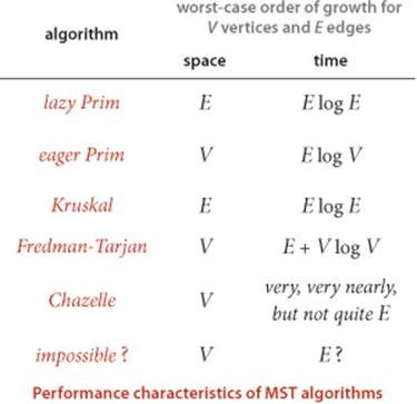
Proposition M. The lazy version of Prim’s algorithm uses space proportional to E and time proportional to E log E (in the worst case) to compute the MST of a connected edge-weighted graph with E edges and V vertices.
Proof: The bottleneck in the algorithm is the number of edge-weight comparisons in the priority-queue methods insert() and delMin(). The number of edges on the priority queue is at most E, which gives the space bound. In the worst case, the cost of an insertion is ~lg E and the cost to delete the minimum is ~2 lg E (see PROPOSITION Q in CHAPTER 2). Since at most E edges are inserted and at most E are deleted, the time bound follows.
In practice, the upper bound on the running time is a bit conservative because the number of edges on the priority queue is typically much less than E. The existence of such a simple, efficient, and useful algorithm for such a challenging task is quite remarkable. Next, we briefly discuss some improvements. As usual, detailed evaluation of such improvements in performance-critical applications is a job for experts.
Lazy version of Prim’s MST algorithm
public class LazyPrimMST
{
private boolean[] marked; // MST vertices
private Queue<Edge> mst; // MST edges
private MinPQ<Edge> pq; // crossing (and ineligible) edges
public LazyPrimMST(EdgeWeightedGraph G)
{
pq = new MinPQ<Edge>();
marked = new boolean[G.V()];
mst = new Queue<Edge>();
visit(G, 0); // assumes G is connected (see Exercise 4.3.22)
while (!pq.isEmpty())
{
Edge e = pq.delMin(); // Get lowest-weight
int v = e.either(), w = e.other(v); // edge from pq.
if (marked[v] && marked[w]) continue; // Skip if ineligible.
mst.enqueue(e); // Add edge to tree.
if (!marked[v]) visit(G, v); // Add vertex to tree
if (!marked[w]) visit(G, w); // (either v or w).
}
}
private void visit(EdgeWeightedGraph G, int v)
{ // Mark v and add to pq all edges from v to unmarked vertices.
marked[v] = true;
for (Edge e : G.adj(v))
if (!marked[e.other(v)]) pq.insert(e);
}
public Iterable<Edge> edges()
{ return mst; }
public double weight() // See Exercise 4.3.31.
}
This implementation of Prim’s algorithm uses a priority queue to hold crossing edges, a vertex-indexed array to mark tree vertices, and a queue to hold MST edges. This implementation is a lazy approach where we leave ineligible edges in the priority queue.
Eager version of Prim’s algorithm
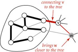
To improve the LazyPrimMST, we might try to delete ineligible edges from the priority queue, so that the priority queue contains only the crossing edges between tree vertices and non-tree vertices. But we can eliminate even more edges. The key is to note that our only interest is in the minimaledge from each non-tree vertex to a tree vertex. When we add a vertex v to the tree, the only possible change with respect to each non-tree vertex w is that adding v brings w closer than before to the tree. In short, we do not need to keep on the priority queue all of the edges from w to tree vertices—we just need to keep track of the minimum-weight edge and check whether the addition of v to the tree necessitates that we update that minimum (because of an edge v-w that has lower weight), which we can do as we process each edge in v’s adjacency list. In other words, we maintain on the priority queue just one edge for each non-tree vertex w: the lightest edge that connects it to the tree. Any heavier edge connecting w to the tree will become ineligible at some point, so there is no need to keep it on the priority queue.
PrimMST (ALGORITHM 4.7 on page 622) implements Prim’s algorithm using our index priority queue data type from SECTION 2.4 (see page 320). It replaces the data structure marked[] and mst[] in LazyPrimMST by two vertex-indexed arrays edgeTo[] and distTo[], which have the following properties:
• If v is not on the tree but has at least one edge connecting it to the tree, then edgeTo[v] is the lightest edge connecting v to the tree, and distTo[v] is the weight of that edge.
• All such vertices v are maintained on the index priority queue, as an index v associated with the weight of edgeTo[v].
The key implications of these properties is that the minimum key on the priority queue is the weight of the minimal-weight crossing edge, and its associated vertex v is the next to add to the tree. To maintain the data structures, PrimMST takes a vertex v from the priority queue, then checks each edge v-w on its adjacency list. If w is marked, the edge is ineligible; if it is not on the priority queue or its weight is lower than the current best-known edgeTo[w], the code updates the data structures to establish v-w as the best-known way to connect w to the tree.
The figure on the facing page is a trace of PrimMST for our small sample graph tinyEWG.txt. The contents of the edgeTo[] and distTo[] arrays are depicted after each vertex is added to the MST, color-coded to depict the MST vertices (index in black), the non-MST vertices (index in gray), the MST edges (in black), and the priority-queue index/value pairs (in red). In the drawings, the lightest edge connecting each non-MST vertex to an MST vertex is drawn in red. The algorithm adds edges to the MST in the same order as the lazy version; the difference is in the priority-queue operations. It builds the MST as follows:
• Adds 0 to the MST and all edges in its adjacency list to the priority queue, since each such edge is the best (only) known connection between a tree vertex and a non-tree vertex.
• Adds 7 and 0-7 to the MST, replaces 0-4 with 4-7 as the lighest edge from a tree vertex to 4, adds 1-7 and 5-7 to the priority queue. Edge 2-7 does not affect the priority queue because its weights is not less than the weight of the known connection from the MST to 2.
• Adds 1 and 1-7 to the MST and 1-3 to the priority queue.
• Adds 2 and 0-2 to the MST, replaces 6-0 with 2-6 as the lightest edge from a tree vertex to 6, and replaces 1-3 with 2-3 as the lightest edge from a tree vertex to 3.
• Adds 3 and 2-3 to the MST.
• Adds 5 and 5-7 to the MST and replaces 4-7 with 4-5 as the lightest edge from a tree vertex to 4.
• Adds 4 and 4-5 to the MST.
• Adds 6 and 6-2 to the MST.
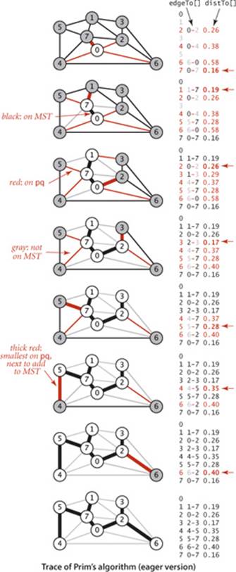
After having added V−1 edges, the MST is complete and the priority queue is empty.
AN ESSENTIALLY IDENTICAL ARGUMENT as in the proof of PROPOSITION M proves that the eager version of Prim’s algorithm finds the MST of a connected edge-weighted graph in time proportional to E log V and extra space proportional to V. For the huge sparse graphs that are typical in practice, there is no asymptotic difference in the time bound (because lg E ~ lg V for sparse graphs); the space bound is a constant-factor (but significant) improvement. Further analysis and experimentation are best left for experts facing performance-critical applications, where many factors come into play, including the implementations of MinPQ and IndexMinPQ, the graph representation, properties of the application’s graph model, and so forth. As usual, such improvements need to be carefully considered, as the increased code complexity is only justified for applications where constant-factor performance gains are important, and might even be counterproductive on complex modern systems.
Algorithm 4.7 Prim’s MST algorithm (eager version)
public class PrimMST
{
private Edge[] edgeTo; // shortest edge from tree vertex
private double[] distTo; // distTo[w] = edgeTo[w].weight()
private boolean[] marked; // true if v on tree
private IndexMinPQ<Double> pq; // eligible crossing edges
public PrimMST(EdgeWeightedGraph G)
{
edgeTo = new Edge[G.V()];
distTo = new double[G.V()];
marked = new boolean[G.V()];
for (int v = 0; v < G.V(); v++)
distTo[v] = Double.POSITIVE_INFINITY;
pq = new IndexMinPQ<Double>(G.V());
distTo[0] = 0.0;
pq.insert(0, 0.0); // Initialize pq with 0, weight 0.
while (!pq.isEmpty())
visit(G, pq.delMin()); // Add closest vertex to tree.
}
private void visit(EdgeWeightedGraph G, int v)
{ // Add v to tree; update data structures.
marked[v] = true;
for (Edge e : G.adj(v))
{
int w = e.other(v);
if (marked[w]) continue; // v-w is ineligible.
if (e.weight() < distTo[w])
{ // Edge e is new best connection from tree to w.
edgeTo[w] = e;
distTo[w] = e.weight();
if (pq.contains(w)) pq.changeKey(w, distTo[w]);
else pq.insert(w, distTo[w]);
}
}
}
public Iterable<Edge> edges() // See Exercise 4.3.21.
public double weight() // See Exercise 4.3.31.
}
This implementation of Prim’s algorithm keeps eligible crossing edges on an index priority queue.
Proposition N. The eager version of Prim’s algorithm uses extra space proportional to V and time proportional to E log V (in the worst case) to compute the MST of a connected edge-weighted graph with E edges and V vertices.
Proof: The number of vertices on the priority queue is at most V, and there are three vertex-indexed arrays, which implies the space bound. The algorithm uses V insert operations, V delete the minimum operations, and (in the worst case) E change priority operations. These counts, coupled with the fact that our heap-based implementation of the index priority queue implements all these operations in time proportional to log V (see page 321), imply the time bound.
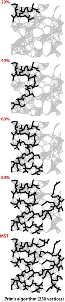
The diagram at right shows Prim’s algorithm in operation on our 250-vertex Euclidean graph mediumEWG.txt. It is a fascinating dynamic process (see also EXERCISE 4.3.27). Most often the tree grows by connecting a new vertex to the vertex just added. When reaching an area with no nearby non-tree vertices, the growth starts from another part of the tree.
Kruskal’s algorithm
The second MST algorithm that we consider in detail is to process the edges in order of their weight values (smallest to largest), taking for the MST (coloring black) each edge that does not form a cycle with edges previously added, stopping after adding V−1 edges. The black edges form a forest of trees that evolves gradually into a single tree, the MST. This method is known as Kruskal’s algorithm:
Proposition O. Kruskal’s algorithm computes the MST of any connected edge-weighted graph.
Proof: Immediate from PROPOSITION K. If the next edge to be considered does not form a cycle with black edges, it crosses a cut defined by the set of vertices connected to one of the edge’s vertices by black edges (and its complement). Since the edge does not create a cycle, it is the only crossing edge seen so far, and since we consider the edges in sorted order, it is a crossing edge of minimum weight. Thus, the algorithm is successively taking a minimal-weight crossing edge, in accordance with the greedy algorithm.
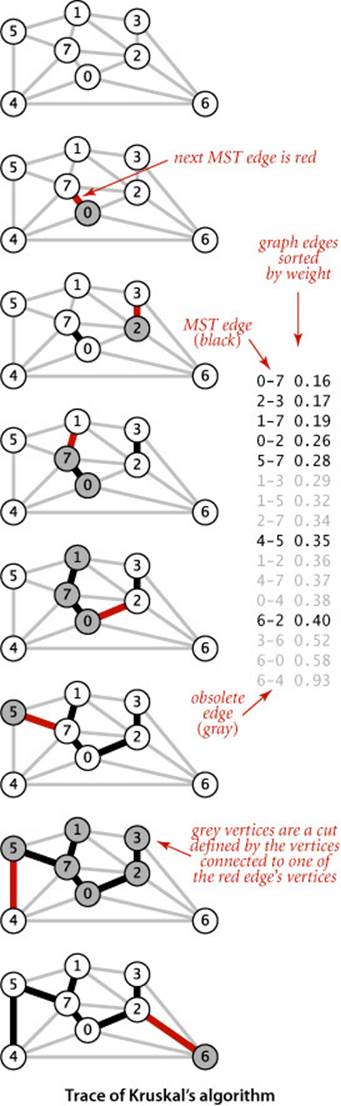
Prim’s algorithm builds the MST one edge at a time, finding a new edge to attach to a single growing tree at each step. Kruskal’s algorithm also builds the MST one edge at a time; but, by contrast, it finds an edge that connects two trees in a forest of growing trees. We start with a degenerate forest of V single-vertex trees and perform the operation of combining two trees (using the lightest edge possible) until there is just one tree left: the MST.
The figure at left shows a step-by-step example of the operation of Kruskal’s algorithm on tinyEWG.txt. The five lowest-weight edges in the graph are taken for the MST, then 1-3, 1-5, and 2-7 are determined to be ineligible before 4-5 is taken for the MST, and finally 1-2, 4-7, and 0-4 are determined to be ineligible and 6-2 is taken for the MST.
Kruskal’s algorithm is also not difficult to implement, given the basic algorithmic tools that we have considered in this book: we use a priority queue (SECTION 2.4) to consider the edges in order by weight, a union-find data structure (SECTION 1.5) to identify those that cause cycles, and a queue (SECTION 1.3) to collect the MST edges. ALGORITHM 4.8 is an implementation along these lines. Note that collecting the MST edges in a Queue means that when a client iterates through the edges it gets them in increasing order of their weight. The weight() method requires iterating through the queue to add the edge weights (or keeping a running total in an instance variable) and is left as an exercise (see EXERCISE 4.3.31).
Analyzing the running time of Kruskal’s algorithm is a simple matter because we know the running times of its basic operations.
Proposition N (continued). Kruskal’s algorithm uses space proportional to E and time proportional to E log E (in the worst case) to compute the MST of an edge-weighted connected graph with E edges and V vertices.
Proof: The implementation uses the priority-queue constructor that initializes the priority queue with all the edges, at a cost of at most E compares (see SECTION 2.4). After the priority queue is built, the argument is the same as for Prim’s algorithm. The number of edges on the priority queue is at most E, which gives the space bound, and the cost per operation is at most 2 lg E compares, which gives the time bound. Kruskal’s algorithm also performs up to E find() and V union() operations, but that cost does not contribute to the E log E order of growth of the total running time (see SECTION 1.5).
As with Prim’s algorithm the cost bound is conservative, since the algorithm terminates after finding the V−1 MST edges. The order of growth of the actual cost is E + E0 log E, where E0 is the number of edges whose weight is less than the weight of the MST edge with the highest weight. Despite this advantage, Kruskal’s algorithm is generally slower than Prim’s algorithm because it has to do a connected() operation for each edge, in addition to the priority-queue operations that both algorithms do for each edge processed (see EXERCISE 4.3.39).
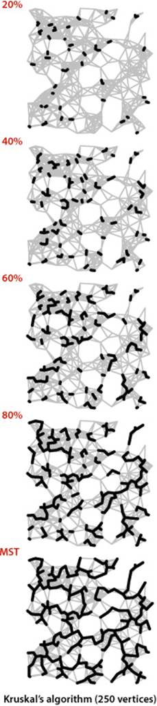
The figure at left illustrates the algorithm’s dynamic characteristics on the larger example mediumEWG.txt. The fact that the edges are added to the forest in order of their length is quite apparent.
Algorithm 4.8 Kruskal’s MST algorithm
public class KruskalMST
{
private Queue<Edge> mst;
public KruskalMST(EdgeWeightedGraph G)
{
mst = new Queue<Edge>();
MinPQ<Edge> pq = new MinPQ<Edge>();
for (Edge e : G.edges())
pq.insert(e);
UF uf = new UF(G.V());
while (!pq.isEmpty() && mst.size() < G.V()-1)
{
Edge e = pq.delMin(); // Get min weight edge on pq
int v = e.either(), w = e.other(v); // and its vertices.
if (uf.connected(v, w)) continue; // Ignore ineligible edges.
uf.union(v, w); // Merge components.
mst.enqueue(e); // Add edge to mst.
}
}
public Iterable<Edge> edges()
{ return mst; }
public double weight() // See Exercise 4.3.31.
}
This implementation of Kruskal’s algorithm uses a queue to hold MST edges, a priority queue to hold edges not yet examined, and a union-find data structure for identifying ineligible edges. The MST edges are returned to the client in increasing order of their weights. The weight()method is left as an exercise.
% java KruskalMST tinyEWG.txt
0-7 0.16000
2-3 0.17000
1-7 0.19000
0-2 0.26000
5-7 0.28000
4-5 0.35000
6-2 0.40000
1.8100
Perspective
The MST problem is one of the most heavily studied problems that we encounter in this book. Basic approaches to solving it were invented long before the development of modern data structures and modern techniques for analyzing the performance of algorithms, at a time when finding the MST of a graph that contained, say, thousands of edges was a daunting task. The MST algorithms that we have considered differ from these old ones essentially in their use and implementation of modern algorithms and data structures for basic tasks, which (coupled with modern computing power) makes it possible for us to compute MSTs with millions or even billions of edges.
Historical notes
An MST implementation for dense graphs (see EXERCISE 4.3.29) was first presented by R. Prim in 1961 and, independently, by E. W. Dijkstra soon thereafter. It is usually referred to as Prim’s algorithm, although Dijkstra’s presentation was more general. But the basic idea was also presented by V. Jarnik in 1939, so some authors refer to the method as Jarnik’s algorithm, thus characterizing Prim’s (or Dijkstra’s) role as finding an efficient implementation of the algorithm for dense graphs. As the priority-queue ADT came into use in the early 1970s, its application to finding MSTs of sparse graphs was straightforward; the fact that MSTs of sparse graphs could be computed in time proportional to E log E became widely known without attribution to any particular researcher. In 1984, M. L. Fredman and R. E. Tarjan developed the Fibonacci heap data structure, which improves the theoretical bound on the order of growth of the running time of Prim’s algorithm to E + V log V. J. Kruskal presented his algorithm in 1956, but, again, the relevant ADT implementations were not carefully studied for many years. Other interesting historical notes are that Kruskal’s paper mentioned a version of Prim’s algorithm and that a 1926 (!) paper by O. Boruvka mentioned both approaches. Boruvka’s paper addressed a power-distribution application and introduced yet another method that is easily implemented with modern data structures (see EXERCISE 4.3.43 and EXERCISE 4.3.44). The method was rediscovered by M. Sollin in 1961; it later attracted attention as the basis for MST algorithms with efficient asymptotic performance and as the basis for parallel MST algorithms.
A linear-time algorithm?
On the one hand, no theoretical results have been developed that deny the existence of an MST algorithm that is guaranteed to run in linear time for all graphs. On the other hand, the goal of developing algorithms for computing the MST of sparse graphs in linear time remains elusive. Since the 1970s the applicability of the union-find abstraction to Kruskal’s algorithm and the applicability of the priority-queue abstraction to Prim’s algorithm have been prime motivations for many researchers to seek better implementations of those ADTs. Many researchers have concentrated on finding efficient priority-queue implementations as the key to finding efficient MST algorithms for sparse graphs; many other researchers have studied variations of Boruvka’s algorithm as the basis for nearly linear-time MST algorithms for sparse graphs. Such research still holds the potential to lead us eventually to a practical linear-time MST algorithm and has even shown the existence of a randomized linear-time algorithm. Also, researchers are getting quite close to the linear-time goal: B. Chazelle exhibited an algorithm in 1997 that certainly could never be distinguished from a linear-time algorithm in any conceivable practical situation (even though it is provably nonlinear), but is so complicated that no one would use it in practice. While the algorithms that have emerged from such research are generally quite complicated, simplified versions of some of them may yet be shown to be useful in practice. In the meantime, we can use the basic algorithms that we have considered here to compute the MST in linear time in most practical situations, perhaps paying an extra factor of log V for some sparse graphs.
IN SUMMARY, we can consider the MST problem to be “solved” for practical purposes. For most graphs, the cost of finding the MST is only slightly higher than the cost of extracting the graph’s edges. This rule holds except for huge graphs that are extremely sparse, but the available performance improvement over the best-known algorithms even in this case is a small constant factor, perhaps a factor of 10 at best. These conclusions are borne out for many graph models, and practitioners have been using Prim’s and Kruskal’s algorithms to find MSTs in huge graphs for decades.
Q&A
Q. Do Prim’s and Kruskal’s algorithms work for directed graphs?
A. No, not at all. That is a more difficult graph-processing problem known as the minimum cost arborescence problem.
Exercises
4.3.1 Prove that you can rescale the weights by adding a positive constant to all of them or by multiplying them all by a positive constant without affecting the MST.
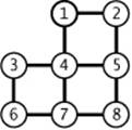
4.3.2 Draw all of the MSTs of the graph depicted at right (all edge weights are equal).
4.3.3 Show that if a graph’s edges all have distinct weights, the MST is unique.
4.3.4 Consider the assertion that an edge-weighted graph has a unique MST only if its edge weights are distinct. Give a proof or a counterexample.
4.3.5 Show that the greedy algorithm is valid even when edge weights are not distinct.
4.3.6 Give the MST of the weighted graph obtained by deleting vertex 7 from tinyEWG.txt (see page 604).
4.3.7 How would you find a maximum spanning tree of an edge-weighted graph?
4.3.8 Prove the following, known as the cycle property: Given any cycle in an edge-weighted graph (all edge weights distinct), the edge of maximum weight in the cycle does not belong to the MST of the graph.
4.3.9 Implement the constructor for EdgeWeightedGraph that reads an edge-weighted graph from the input stream, by suitably modifying the constructor from Graph (see page 526).
4.3.10 Develop an EdgeWeightedGraph implementation for dense graphs that uses an adjacency-matrix (two-dimensional array of weights) representation. Disallow parallel edges.
4.3.11 Determine the amount of memory used by EdgeWeightedGraph to represent a graph with V vertices and E edges, using the memory-cost model of SECTION 1.4.
4.3.12 Suppose that a graph has distinct edge weights. Does its lightest edge have to belong to the MST? Can its heaviest edge belong to the MST? Does a min-weight edge on every cycle have to belong to the MST? Prove your answer to each question or give a counterexample.
4.3.13 Give a counterexample that shows why the following strategy does not necessarily find the MST: ‘Start with any vertex as a single-vertex MST, then add V-1 edges to it, always taking next a min-weight edge incident to the vertex most recently added to the MST.’
4.3.14 Given an MST for an edge-weighted graph G, suppose that an edge in G that does not disconnect G is deleted. Describe how to find an MST of the new graph in time proportional to E.
4.3.15 Given an MST for an edge-weighted graph G and a new edge e with weight w, describe how to find an MST of the new graph in time proportional to V.
4.3.16 Given an MST for an edge-weighted graph G and a new edge e, write a program that determines the range of weights for which e is in an MST.
4.3.17 Implement toString() for EdgeWeightedGraph.
4.3.18 Give traces that show the process of computing the MST of the graph defined in EXERCISE 4.3.6 with the lazy version of Prim’s algorithm, the eager version of Prim’s algorithm, and Kruskal’s algorithm.
4.3.19 Suppose that you implement PrimMST but instead of using a priority queue to find the next vertex to add to the tree, you scan through all V entries in the distTo[] array to find the non-tree vertex with the smallest weight. What would be the order of growth of the running time for graphs with V vertices and E edges? When would this method be appropriate, if ever? Defend your answer.
4.3.20 True or false: At any point during the execution of Kruskal’s algorithm, each vertex is closer to some vertex in its subtree than to any vertex not in its subtree. Prove your answer.
4.3.21 Provide an implementation of edges() for PrimMST (page 622).
Solution:
public Iterable<Edge> edges()
{
Queue<Edge> mst = new Queue<Edge>();
for (int v = 1; v < edgeTo.length; v++)
mst.enqueue(edgeTo[v]);
return mst;
}
Creative Problems
4.3.22 Minimum spanning forest. Develop versions of Prim’s and Kruskal’s algorithms that compute the minimum spanning forest of an edge-weighted graph that is not necessarily connected. Use the connected-components API of SECTION 4.1 and find MSTs in each component.
4.3.23 Vyssotsky’s algorithm. Develop an implementation that computes the MST by applying the cycle property (see EXERCISE 4.3.8) repeatedly: Add edges one at a time to a putative tree, deleting a maximum-weight edge on the cycle if one is formed. Note: This method has received less attention than the others that we consider because of the comparative difficulty of maintaining a data structure that supports efficient implementation of the “delete the maximum-weight edge on the cycle” operation.
4.3.24 Reverse-delete algorithm. Develop an implementation that computes the MST as follows: Start with a graph containing all of the edges. Then repeatedly go through the edges in decreasing order of weight. For each edge, check if deleting that edge will disconnect the graph; if not, delete it. Prove that this algorithm computes the MST. What is the order of growth of the number of edge-weight compares performed by your implementation?
4.3.25 Worst-case generator. Develop a reasonable generator for edge-weighted graphs with V vertices and E edges such that the running time of the lazy version of Prim’s algorithm is nonlinear. Answer the same question for the eager version.
4.3.26 Critical edges. An MST edge whose deletion from the graph would cause the MST weight to increase is called a critical edge. Show how to find all critical edges in a graph in time proportional to E log E. Note: This question assumes that edge weights are not necessarily distinct (otherwise all edges in the MST are critical).
4.3.27 Animations. Write a client program that does dynamic graphical animations of MST algorithms. Run your program for mediumEWG.txt to produce images like the figures on page 621 and page 624.
4.3.28 Space-efficient data structures. Develop an implementation of the lazy version of Prim’s algorithm that saves space by using lower-level data structures for EdgeWeightedGraph and for MinPQ instead of Bag and Edge. Estimate the amount of memory saved as a function of V and E, using the memory-cost model of SECTION 1.4 (see EXERCISE 4.3.11).
4.3.29 Dense graphs. Develop an implementation of Prim’s algorithm that uses an eager approach (but not a priority queue) and computes the MST using V2 edge-weight comparisons.
4.3.30 Euclidean weighted graphs. Modify your solution to EXERCISE 4.1.37 to create an API EuclideanEdgeWeightedGraph for graphs whose vertices are points in the plane, so that you can work with graphical representations.
4.3.31 MST weights. Develop implementations of weight() for LazyPrimMST, PrimMST, and KruskalMST, using a lazy strategy that iterates through the MST edges when the client calls weight(). Then develop alternate implementations that use an eager strategy that maintains a running total as the MST is computed.
4.3.32 Specified set. Given a connected edge-weighted graph G and a specified set of edges S (having no cycles), describe a way to find a minimum-weight spanning tree of G among those spanning trees that contain all the edges in S.
4.3.33 Certification. Write an MST and EdgeWeightedGraph client check() that uses the following cut optimality conditions implied by PROPOSITION J to verify that a proposed set of edges is in fact an MST: A set of edges is an MST if it is a spanning tree and every edge is a minimum-weight edge in the cut defined by removing that edge from the tree. What is the order of growth of the running time of your method?
Experiments
4.3.34 Random sparse edge-weighted graphs. Write a random-sparse-edge-weighted-graph generator based on your solution to EXERCISE 4.1.41. To assign edge weights, define a random-edge-weighted graph ADT and write two implementations: one that generates uniformly distributed weights, another that generates weights according to a Gaussian distribution. Write client programs to generate sparse random edge-weighted graphs for both weight distributions with a well-chosen set of values of V and E so that you can use them to run empirical tests on graphs drawn from various distributions of edge weights.
4.3.35 Random Euclidean edge-weighted graphs. Modify your solution to EXERCISE 4.1.42 to assign the distance between vertices as each edge’s weight.
4.3.36 Random grid edge-weighted graphs. Modify your solution to EXERCISE 4.1.43 to assign a random weight (between 0 and 1) to each edge.
4.3.37 Real edge-weighted graphs. Find a large weighted graph somewhere online—perhaps a map with distances, telephone connections with costs, or an airline rate schedule. Write a program RandomRealEdgeWeightedGraph that builds a weighted graph by choosing V vertices at random and Eweighted edges at random from the subgraph induced by those vertices.
Testing all algorithms and studying all parameters against all graph models is unrealistic. For each problem listed below, write a client that addresses the problem for any given input graph, then choose among the generators above to run experiments for that graph model. Use your judgment in selecting experiments, perhaps in response to results of previous experiments. Write a narrative explaining your results and any conclusions that might be drawn.
4.3.38 Cost of laziness. Run empirical studies to compare the performance of the lazy version of Prim’s algorithm with the eager version, for various types of graphs.
4.3.39 Prim versus Kruskal. Run empirical studies to compare the performance of the lazy and eager versions of Prim’s algorithm with Kruskal’s algorithm.
4.3.40 Reduced overhead. Run empirical studies to determine the effect of using primitive types instead of Edge values in EdgeWeightedGraph, as described in EXERCISE 4.3.28.
4.3.41 Heaviest MST edge. Run empirical studies to analyze the weight of the heaviest edge in the MST and the number of graph edges that are not heavier than that one.
4.3.42 Partitioning. Develop an implementation based on integrating Kruskal’s algorithm with quicksort partitioning (instead of using a priority queue) so as to check MST membership of each edge as soon as all smaller edges have been checked.
4.3.43 Boruvka’s algorithm. Develop an implementation of Boruvka’s algorithm: Build an MST by adding edges to a growing forest of trees, as in Kruskal’s algorithm, but in stages. At each stage, find the minimum-weight edge that connects each tree to a different one, then add all such edges to the MST. Assume that the edge weights are all different, to avoid cycles. Hint: Maintain a vertex-indexed array to identify the edge that connects each tree to its nearest neighbor, and use the union-find data structure.
4.3.44 Improved Boruvka. Develop an implementation of Boruvka’s algorithm that uses doubly-linked circular lists to represent MST subtrees so that subtrees can be merged and renamed in time bounded by E during each stage (and the union-find data type is therefore not needed).
4.3.45 External MST. Describe how you would find the MST of a graph so large that only V edges can fit into main memory at once.
4.3.46 Johnson’s algorithm. Develop a priority-queue implementation that uses a d-way heap (see EXERCISE 2.4.41). Find the best value of d for various weighted graph models.
All materials on the site are licensed Creative Commons Attribution-Sharealike 3.0 Unported CC BY-SA 3.0 & GNU Free Documentation License (GFDL)
If you are the copyright holder of any material contained on our site and intend to remove it, please contact our site administrator for approval.
© 2016-2026 All site design rights belong to S.Y.A.