Algorithms (2014)
Five. Strings
5.5 Data Compression
The world is awash with data, and algorithms designed to represent data efficiently play an important role in the modern computational infrastructure. There are two primary reasons to compress data: to save storage when saving information and to save time when communicating information. Both of these reasons have remained important through many generations of technology and are familiar today to anyone needing a new storage device or waiting for a long download.
You have certainly encountered compression when working with digital images, sound, movies, and all sorts of other data. The algorithms we will examine save space by exploiting the fact that most data files have a great deal of redundancy: For example, text files have certain character sequences that appear much more often than others; bitmap files that encode pictures have large homogeneous areas; and files for the digital representation of images, movies, sound, and other analog signals have large repeated patterns.
We will look at an elementary algorithm and two advanced methods that are widely used. The compression achieved by these methods varies depending on characteristics of the input. Savings of 20 to 50 percent are typical for text, and savings of 50 to 90 percent might be achieved in some situations. As you will see, the effectiveness of any data compression method is quite dependent on characteristics of the input. Note: Usually, in this book, we are referring to time when we speak of performance; with data compression we normally are referring to the compression they can achieve, although we will also pay attention to the time required to do the job.
On the one hand, data-compression techniques are less important than they once were because the cost of computer storage devices has dropped dramatically and far more storage is available to the typical user than in the past. On the other hand, data-compression techniques are more important than ever because, since so much storage is in use, the savings they make possible are greater. Indeed, data compression has come into widespread use with the emergence of the internet, because it is a low-cost way to reduce the time required to transmit large amounts of data.
Data compression has a rich history (we will only be providing a brief introduction to the topic), and contemplating its role in the future is certainly worthwhile. Every student of algorithms can benefit from studying data compression because the algorithms are classic, elegant, interesting, and effective.
Rules of the game
All of the types of data that we process with modern computer systems have something in common: they are ultimately represented in binary. We can consider each of them to be simply a sequence of bits (or bytes). For brevity, we use the term bitstream in this section to refer to a sequence of bits and bytestream when we are referring to the bits being considered as a sequence of fixed-size bytes. A bitstream or a bytestream might be stored as a file on your computer, or it might be a message being transmitted on the internet.
Basic model
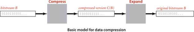
Accordingly, our basic model for data compression is quite simple, having two primary components, each a black box that reads and writes bitstreams:
• A compress box that transforms a bitstream B into a compressed version C (B)
• An expand box that transforms C (B) back into B
Using the notation | B | to denote the number of bits in a bitstream, we are interested in minimizing the quantity | C(B) | / | B |, which is known as the compression ratio.
This model is known as lossless compression—we insist that no information be lost, in the specific sense that the result of compressing and expanding a bitstream must match the original, bit for bit. Lossless compression is required for many types of files, such as numerical data or executable code. For some types of files (such as images, videos, or music), it is reasonable to consider compression methods that are allowed to lose some information, so the decoder only produces an approximation of the original file. Lossy methods have to be evaluated in terms of a subjective quality standard in addition to the compression ratio. We do not address lossy compression in this book.
Reading and writing binary data
A full description of how information is encoded on your computer is system-dependent and is beyond our scope, but with a few basic assumptions and two simple APIs, we can separate our implementations from these details. These APIs, BinaryStdIn and BinaryStdOut, are modeled on the StdInand StdOut APIs that you have been using, but their purpose is to read and write bits, where StdIn and StdOut are oriented toward character streams encoded in Unicode. An int value on StdOut is a sequence of characters (its decimal representation); an int value on BinaryStdOut is a sequence of bits (its binary representation).
Binary input and output
Most systems nowadays, including Java, base their I/O on 8-bit bytestreams, so we might decide to read and write bytestreams to match I/O formats with the internal representations of primitive types, encoding an 8-bit char with 1 byte, a 16-bit short with 2 bytes, a 32-bit int with 4 bytes, and so forth. Since bitstreams are the primary abstraction for data compression, we go a bit further to allow clients to read and write individual bits, intermixed with data of primitive types. The goal is to minimize the necessity for type conversion in client programs and also to take care of operating system conventions for representing data. We use the following API for reading a bitstream from standard input:
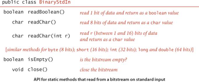
A key feature of the abstraction is that, in marked constrast to StdIn, the data on standard input is not necessarily aligned on byte boundaries. If the input stream is a single byte, a client could read it 1 bit at a time with eight calls to readBoolean(). The close() method is not essential, but, for clean termination, clients should call close() to indicate that no more bits are to be read. As with StdIn/StdOut, we use the following complementary API for writing bitstreams to standard output:
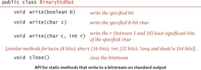
For output, the close() method is essential: clients must call close() to ensure that all of the bits specified in prior write() calls make it to the bitstream and that the final byte is padded with 0s to byte-align the output for compatibility with the file system. As with the In and Out APIs associated with StdIn and StdOut, we also have available BinaryIn and BinaryOut that allows us to reference binary-encoded files directly.
Example
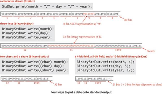
As a simple example, suppose that you have a data type where a date is represented as three int values (month, day, year). Using StdOut to write those values in the format 12/31/1999 requires 10 characters, or 80 bits. If you write the values directly with BinaryStdOut, you would produce 96 bits (32 bits for each of the 3 int values); if you use a more economical representation that uses byte values for the month and day and a short value for the year, you would produce 32 bits. With BinaryStdOut you could also write a 4-bit field, a 5-bit field, and a 12-bit field, for a total of 21 bits (24 bits, actually, because files must be an integral number of 8-bit bytes, so close() adds three 0 bits at the end). Important note: Such economy, in itself, is a crude form of data compression.
Binary dumps
How can we examine the contents of a bitstream or a bytestream while debugging? This question faced early programmers when the only way to find a bug was to examine each of the bits in memory, and the term dump has been used since the early days of computing to describe a human-readable view of a bitstream. If you try to open a file with an editor or view it in the manner in which you view text files (or just run a program that uses BinaryStdOut), you are likely to see gibberish, depending on the system you use. BinaryStdIn allows us to avoid such system dependencies by writing our own programs to convert bitstreams such that we can see them with our standard tools. For example, the program BinaryDump at left is a BinaryStdIn client that prints out the bits from standard input, encoded with the characters 0 and 1. This program is useful for debugging when working with small inputs. The similar client HexDump groups the data into 8-bit bytes and prints each as two hexadecimal digits that each represent 4 bits. The client PictureDump displays the bits in a Picture with 0 bits represented as white pixels and 1 bits represented as black pixels. This pictorial representation is often useful in identifying patterns in a bitstream. You can download BinaryDump, HexDump, and PictureDump from the booksite. Typically, we use piping and redirection at the command-line level when working with binary files: we can pipe the output of an encoder to BinaryDump, HexDump, or PictureDump, or redirect it to a file.
Printing a bitstream on standard (character) output
public class BinaryDump
{
public static void main(String[] args)
{
int width = Integer.parseInt(args[0]);
int cnt;
for (cnt = 0; !BinaryStdIn.isEmpty(); cnt++)
{
if (width == 0) continue;
if (cnt != 0 && cnt % width == 0)
StdOut.println();
if (BinaryStdIn.readBoolean())
StdOut.print("1");
else StdOut.print("0");
}
StdOut.println();
StdOut.println(cnt + " bits");
}
}
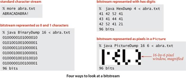
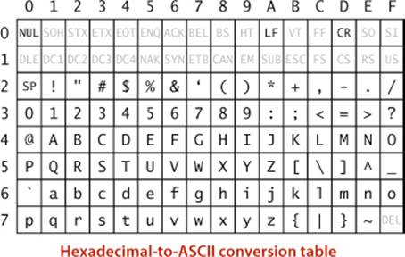
ASCII encoding
When you HexDump a bit-stream that contains ASCII-encoded characters, the table at right is useful for reference. Given a two digit hex number, use the first hex digit as a row index and the second hex digit as a column index to find the character that it encodes. For example, 31 encodes the digit1, 4A encodes the letter J, and so forth. This table is for 7-bit ASCII, so the first hex digit must be 7 or less. Hex numbers starting with 0 and 1 (and the numbers 20 and 7F) correspond to non-printing control characters. Many of the control characters are left over from the days when physical devices such as typewriters were controlled by ASCII input; the table highlights a few that you might see in dumps. For example, SP is the space character, NUL is the null character, LF is line feed, and CR is carriage return.
IN SUMMARY, working with data compression requires us to reorient our thinking about standard input and standard output to include binary encoding of data. BinaryStdIn and BinaryStdOut provide the methods that we need. They provide a way for you to make a clear distinction in your client programs between writing out information intended for file storage and data transmission (that will be read by programs) and printing information (that is likely to be read by humans).
Limitations
To appreciate data-compression algorithms, you need to understand fundamental limitations. Researchers have developed a thorough and important theoretical basis for this purpose, which we will consider briefly at the end of this section, but a few ideas will help us get started.
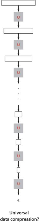
Universal data compression
Armed with the algorithmic tools that have proven so useful for so many problems, you might think that our goal should be universal data compression: an algorithm that can make any bitstream smaller. Quite to the contrary, we have to adopt more modest goals because universal data compression is impossible.
Proposition S. No algorithm can compress every bitstream.
Proof: We consider two proofs that each provide some insight. The first is by contradiction: Suppose that you have an algorithm that does compress every bitstream. Then you could use that algorithm to compress its output to get a still shorter bitstream, and continue until you have a bistream of length 0! The conclusion that your algorithm compresses every bit-stream to 0 bits is absurd, and so is the assumption that it can compress every bitstream.
The second proof is a counting argument. Suppose that you have an algorithm that claims lossless compression for every 1,000-bit stream. That is, every such stream must map to a different shorter one. But there are only 1 + 2 + 4 + ... + 2998 + 2999 = 21000−1 bitstreams with fewer than 1,000 bits and 21000 bitstreams with 1,000 bits, so your algorithm cannot compress all of them. This argument becomes more persuasive if we consider stronger claims. Say your goal is to achieve better than a 50 percent compression ratio. You have to know that you will be successful for only about 1 out of 2500 of the 1,000-bit bitstreams!
Put another way, you have at most a 1 in 2500 chance of being able to compress by half a random 1,000-bit stream with any data-compression algorithm. When you run across a new lossless compression algorithm, it is a sure bet that it will not achieve significant compression for a random bitstream. The insight that we cannot hope to compress random streams is a start to understanding data compression. We regularly process strings of millions or billions of bits but will never process even the tiniest fraction of all possible such strings, so we need not be discouraged by this theoretical result. Indeed, the bitstrings that we regularly process are typically highly structured, a fact that we can exploit for compression.
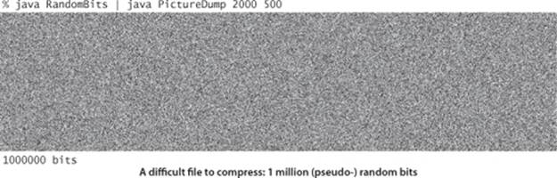
Undecidability
Consider the million-bit string pictured at the top of this page. This string appears to be random, so you are not likely to find a lossless compression algorithm that will compress it. But there is a way to represent that string with just a few thousand bits, because it was produced by the program below. (This program is an example of a pseudo-random number generator, like Java’s Math.random() method.) A compression algorithm that compresses by writing the program in ASCII and expands by reading the program and then running it achieves a .3 percent compression ratio, which is difficult to beat (and we can drive the ratio arbitrarily low by writing more bits). To compress such a file is to discover the program that produced it. This example is not so far-fetched as it first appears: when you compress a video or an old book that was digitized with a scanner or any of countless other types of files from the web, you are discovering something about the program that produced the file. The realization that much of the data that we process is produced by a program leads to deep issues in the theory of computation and also gives insight into the challenges of data compression. For example, it is possible to prove that optimal data compression (find the shortest program to produce a given string) is an undecidable problem: not only can we not have an algorithm that compresses every bit-stream, but also we cannot have a strategy for developing the best algorithm!
A “compressed” million-bit stream
public class RandomBits
{
public static void main(String[] args)
{
int x = 11111;
for (int i = 0; i < 1000000; i++)
{
x = x * 314159 + 218281;
BinaryStdOut.write(x > 0);
}
BinaryStdOut.close();
}
}
The practical impact of these limitations is that lossless compression methods must be oriented toward taking advantage of known structure in the bitstreams to be compressed. The four methods that we consider exploit, in turn, the following structural characteristics:
• Small alphabets
• Long sequences of identical bits/characters
• Frequently used characters
• Long reused bit/character sequences
If you know that a given bitstream exhibits one or more of these characteristics, you can compress it with one of the methods that you are about to learn; if not, trying them each is probably still worth the effort, since the underlying structure of your data may not be obvious, and these methods are widely applicable. As you will see, each method has parameters and variations that may need to be tuned for best compression of a particular bitstream. The first and last recourse is to learn something about the structure of your data yourself and exploit that knowledge to compress it, perhaps using one of the techniques we are about to consider.
Warmup: genomics
As preparation for more complicated data-compression algorithms, we now consider an elementary (but very important) data-compression task. All of our implementations will use the same conventions that we will now introduce in the context of this example.
Genomic data
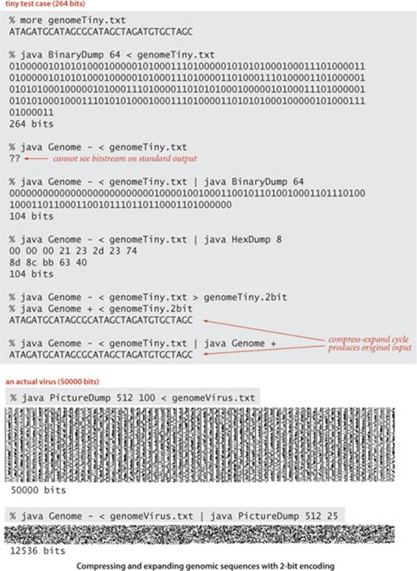
As a first example of data compression, consider this string:
ATAGATGCATAGCGCATAGCTAGATGTGCTAGCAT
Using standard ASCII encoding (1 byte, or 8 bits per character), this string is a bitstream of length 8×35 = 280. Strings of this sort are extremely important in modern biology, because biologists use the letters A, C, T, and G to represent the four nucleotides in the DNA of living organisms. Agenome is a sequence of nucleotides. Scientists know that understanding the properties of genomes is a key to understanding the processes that manifest themselves in living organisms, including life, death, and disease. Genomes for many living things are known, and scientists are writing programs to study the structure of these sequences.
Compression method for genomic data
public static void compress()
{
Alphabet DNA = new Alphabet("ACTG");
String s = BinaryStdIn.readString();
int N = s.length();
BinaryStdOut.write(N);
for (int i = 0; i < N; i++)
{ // Write two-bit code for char.
int d = DNA.toIndex(s.charAt(i));
BinaryStdOut.write(d, DNA.lgR());
}
BinaryStdOut.close();
}
2-bit code compression
One simple property of genomes is that they contain only four different characters, so each can be encoded with just 2 bits per character, as in the compress() method shown at right. Even though we know the input stream to be character-encoded, we use BinaryStdIn to read the input, to emphasize adherence to the standard data-compression model (bitstream to bitstream). We include the number of encoded characters in the compressed file, to ensure proper decoding if the last bit does not fall at the end of a byte. Since it converts each 8-bit character to a 2-bit code and just adds 32 bits for the length, this program approaches a 25 percent compression ratio as the number of characters increases.
2-bit code expansion
The expand() method at the top of the next page expands a bitstream produced by this compress() method. As with compression, this method reads a bitstream and writes a bitstream, in accordance with the basic data-compression model. The bitstream that we produce as output is the original input.
THE SAME APPROACH works for other fixed-size alphabets, but we leave this generalization for an (easy) exercise (see EXERCISE 5.5.25).
Expansion method for genomic data
public static void expand()
{
Alphabet DNA = new Alphabet("ACTG");
int w = DNA.lgR();
int N = BinaryStdIn.readInt();
for (int i = 0; i < N; i++)
{ // Read 2 bits; write char.
char c = BinaryStdIn.readChar(w);
BinaryStdOut.write(DNA.toChar(c), 8);
}
BinaryStdOut.close();
}
These methods do not quite adhere to the standard data-compression model, because the compressed bitstream does not contain all the information needed to decode it. The fact that the alphabet is one of the letters A, C, T, or G is agreed upon by the two methods. Such a convention is reasonable in an application such as genomics, where the same code is widely reused. Other situations might require including the alphabet in the encoded message (see EXERCISE 5.5.25). The norm in data compression is to include such costs when comparing methods.
In the early days of genomics, learning a genomic sequence was a long and arduous task, so sequences were relatively short and scientists used standard ASCII encoding to store and exchange them. The experimental process has been vastly streamlined, to the point where known genomes are numerous and lengthy (the human genome is over 1010 bits), and the 75 percent savings achieved by these simple methods is very significant. Is there room for further compression? That is a very interesting question to contemplate, because it is a scientific question: the ability to compress implies the existence of some structure in the data, and a prime focus of modern genomics is to discover structure in genomic data. Standard data-compression methods like the ones we will consider are ineffective with (2-bit-encoded) genomic data, as with random data.
We package compress() and expand() as static methods in the same class, along with a simple driver, as shown at right. To test your understanding of the rules of the game and the basic tools that we use for data compression, make sure that you understand the various commands on the facing page that invoke Genome.compress() and Genome.expand() on our sample data (and their consequences).
Packaging convention for data-compression methods
public class Genome
{
public static void compress()
// See text.
public static void expand()
// See text.
public static void main(String[] args)
{
if (args[0].equals("-")) compress();
if (args[0].equals("+")) expand();
}
}
Run-length encoding
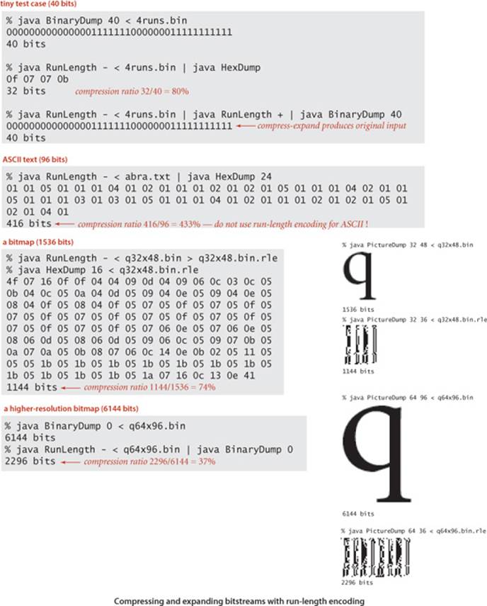
The simplest type of redundancy in a bitstream is long runs of repeated bits. Next, we consider a classic method known as run-length encoding for taking advantage of this redundancy to compress data. For example, consider the following 40-bit string:
0000000000000001111111000000011111111111
This string consists of 15 0s, then 7 1s, then 7 0s, then 11 1s, so we can encode the bitstring with the numbers 15, 7, 7, and 11. All bitstrings are composed of alternating runs of 0s and 1s; we just encode the length of the runs. In our example, if we use 4 bits to encode the numbers and start with a run of 0s, we get the 16-bit string
1111011101111011
(15 = 1111, then 7 = 0111, then 7 = 0111, then 11 = 1011) for a compression ratio of 16/40 = 40 percent. In order to turn this description into an effective data compression method, we have to consider the following issues:
• How many bits do we use to store the counts?
• What do we do when encountering a run that is longer than the maximum count implied by this choice?
• What do we do about runs that are shorter than the number of bits needed to store their length?
We are primarily interested in long bitstreams with relatively few short runs, so we address these questions by making the following choices:
• Counts are between 0 and 255, all encoded with 8 bits.
• We make all run lengths less than 256 by including runs of length 0 if needed.
• We encode short runs, even though doing so might lengthen the output.
These choices are very easy to implement and also very effective for several kinds of bitstreams that are commonly encountered in practice. They are not effective when short runs are numerous—we save bits on a run only when the length of the run is more than the number of bits needed to represent itself in binary.
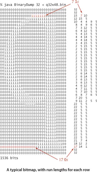
Bitmaps
As an example of the effectiveness of run-length encoding, we consider bitmaps, which are widely use to represent pictures and scanned documents. For brevity and simplicity, we consider binary-valued bitmaps organized as bitstreams formed by taking the pixels in row-major order. To view the contents of a bitmap, we use PictureDump. Writing a program to convert an image from one of the many common lossless image formats that have been defined for “screen shots” or scanned documents into a bitmap is a simple matter. Our example to demonstrate the effectiveness of run-length encoding comes from screen shots of this book: a letter q (at various resolutions). We focus on a binary dump of a 32-by-48-pixel screen shot, shown at right along with run lengths for each row. Since each row starts and ends with a 0, there is an odd number of run lengths on each row; since the end of one row is followed by the beginning of the next, the corresponding run length in the bitstream is the sum of the last run length in each row and the first run length in the next (with extra additions corresponding to rows that are all 0).
Implementation
The informal description just given leads immediately to the compress() and expand() implementations on the next page. As usual, the expand() implementation is the simpler of the two: read a run length, print that many copies of the current bit, complement the current bit, and continue until the input is exhausted. The compress() method is not much more difficult, consisting of the following steps while there are bits in the input stream:
• Read a bit.
• If it differs from the last bit read, write the current count and reset the count to 0.
• If it is the same as the last bit read, and the count is a maximum, write the count, write a 0 count, and reset the count to 0.
• Increment the count.
When the input stream empties, writing the count (length of the last run) completes the process.
Increasing resolution in bitmaps
The primary reason that run-length encoding is widely used for bitmaps is that its effectiveness increases dramatically as resolution increases. It is easy to see why this is true. Suppose that we double the resolution for our example. Then the following facts are evident:
• The number of bits increases by a factor of 4.
• The number of runs increases by about a factor of 2.
• The run lengths increase by about a factor of 2.
• The number of bits in the compressed version increases by about a factor of 2.
• Therefore, the compression ratio is halved!
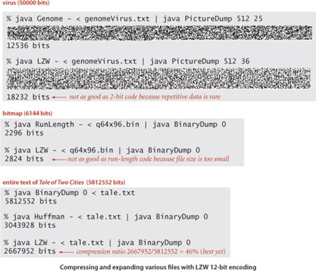
Without run-length encoding, space requirements increase by a factor of 4 when the resolution is doubled; with run-length encoding, space requirements for the compressed bitstream just double when the resolution is doubled. That is, space grows and the compression ratio drops linearly with resolution. For example, our (low-resolution) letter q yields just a 74 percent compression ratio; if we increase the resolution to 64 by 96, the ratio drops to 37 percent. This change is graphically evident in the PictureDump outputs shown in the figure on the facing page. The higher-resolution letter takes four times the space of the lower resolution letter (double in both dimensions), but the compressed version takes just twice the space (double in one dimension). If we further increase the resolution to 128-by-192 (closer to what is needed for print), the ratio drops to 18 percent (seeEXERCISE 5.5.5).
Expand and compress methods for run-length encoding
public static void expand()
{
boolean b = false;
while (!BinaryStdIn.isEmpty())
{
char cnt = BinaryStdIn.readChar();
for (int i = 0; i < cnt; i++)
BinaryStdOut.write(b);
b = !b;
}
BinaryStdOut.close();
}
public static void compress()
{
char cnt = 0;
boolean b, old = false;
while (!BinaryStdIn.isEmpty())
{
b = BinaryStdIn.readBoolean();
if (b != old)
{
BinaryStdOut.writewrite(cnt, 8);
cnt = 0;
old = !old;
}
else
{
if (cnt == 255)
{
BinaryStdOut.write(cnt, 8);
cnt = 0;
BinaryStdOut.write(cnt, 8);
}
}
cnt++;
}
BinaryStdOut.write(cnt);
BinaryStdOut.close();
}
RUN-LENGTH ENCODING IS VERY EFFECTIVE in many situations, but there are plenty of cases where the bitstream we wish to compress (for example, typical English-language text) may have no long runs at all. Next, we consider two methods that are effective for a broad variety of files. They are widely used, and you likely have used one or both of these methods when downloading from the web.
Huffman compression
We now examine a data-compression technique that can save a substantial amount of space in natural language files (and many other kinds of files). The idea is to abandon the way in which text files are usually stored: instead of using the usual 7 or 8 bits for each character, we use fewer bits for characters that appear often than for those that appear rarely.
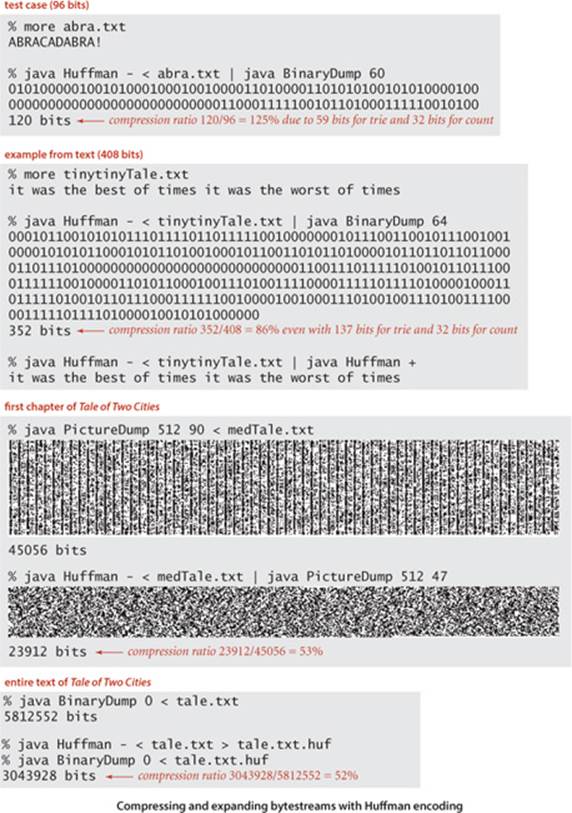
To introduce the basic ideas, we start with a small example. Suppose we wish to encode the string ABRACADABRA! Encoding it in 7-bit ASCII gives this bitstring:
100000110000101010010100000110000111000001-
100010010000011000010101001010000010100001.
To decode this bitstring, we simply read off 7 bits at a time and convert according to the ASCII coding table on page 815. In this standard code the D, which appears only once, requires the same number of bits as the A, which appears five times. Huffman compression is based on the idea that we can save bits by encoding frequently used characters with fewer bits than rarely used characters, thereby lowering the total number of bits used.
Variable-length prefix-free codes
A code associates each character with a bitstring: a symbol table with characters as keys and bitstrings as values. As a start, we might try to assign the shortest bitstrings to the most commonly used letters, encoding A with 0, B with 1, R with 00, C with 01, D with 10, and ! with 11, so ABRACADABRA!would be encoded as 0 1 00 0 01 0 10 0 1 00 0 11. This representation uses only 17 bits compared to the 87 for 7-bit ASCII, but it is not really a code because it depends on the blanks to delimit the characters. Without the blanks, the bitstring would be
01000010100100011
and could be decoded as CRRDDCRCB or as several other strings. Still, the count of 17 bits plus 11 delimiters is rather more compact than the standard code, primarily because no bits are used to encode letters not appearing in the message. The next step is to take advantage of the fact that delimiters are not needed if no character code is the prefix of another. A code with this property is known as a prefix-free code. The code just given is not prefix-free because 0, the code for A, is a prefix of 00, the code for R. For example, if we encode A with 0, B with 1111, C with 110, D with 100, R with 1110, and ! with 101, there is only one way to decode the 30-bit string
011111110011001000111111100101
ABRACADABRA! All prefix-free codes are uniquely decodable (without needing any delimiters) in this way, so prefix-free codes are widely used in practice. Note that fixed-length codes such as 7-bit ASCII are prefix-free.
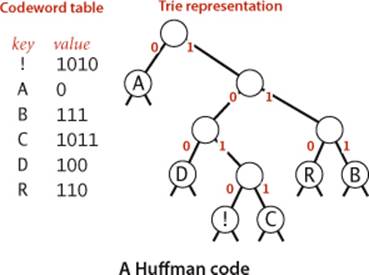
Trie representation for prefix-free codes
One convenient way to represent a prefix-free code is with a trie (see SECTION 5.2). In fact, any trie with M null links defines a prefix-free code for M characters: we replace the null links by links to leaves (nodes with two null links), each containing a character to be encoded, and define the code for each character with the bitstring defined by the path from the root to the character, in the standard manner for tries where we associate 0 with moving left and 1 with moving right. For example, the figure at right shows two prefix-free codes for the characters in ABRACADABRA!. On top is the variable-length code just considered; below is a code that produces the string
11000111101011100110001111101
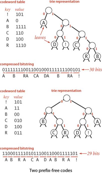
which is 29 bits, 1 bit shorter. Is there a trie that leads to even more compression? How do we find the trie that leads to the best prefix-free code? It turns out that there is an elegant answer to these questions in the form of an algorithm that computes a trie which leads to a bitstream of minimal length for any given string. To make a fair comparison with other codes, we also need to count the bits in the code itself, since the string cannot be decoded without it, and, as you will see, the code depends on the string. The general method for finding the optimal prefix-free code was discovered by D. Huffman (while a student!) in 1952 and is called Huffman encoding.
Overview
Using a prefix-free code for data compression involves five major steps. We view the bitstream to be encoded as a bytestream and use a prefix-free code for the characters as follows:
• Build an encoding trie.
• Write the trie (encoded as a bitstream) for use in expansion.
• Use the trie to encode the bytestream as a bitstream.
Then expansion requires that we
• Read the trie (encoded at the beginning of the bitstream)
• Use the trie to decode the bitstream
To help you best understand and appreciate the process, we consider these steps in order of difficulty.
Trie nodes
We begin with the Node class at left. It is similar to the nested classes that we have used before to construct binary trees and tries: each Node has left and right references to Nodes, which define the trie structure. Each Node also has an instance variable freq that is used in construction, and an instance variable ch, which is used in leaves to represent characters to be encoded.
Trie node representation
private static class Node implements Comparable<Node>
{ // Huffman trie node
private char ch; // unused for internal nodes
private int freq; // unused for expand
private final Node left, right;
Node(char ch, int freq, Node left, Node right)
{
this.ch = ch;
this.freq = freq;
this.left = left;
this.right = right;
}
public boolean isLeaf()
{ return left == null && right == null; }
public int compareTo(Node that)
{ return this.freq - that.freq; }
}
Expansion for prefix-free codes
Expanding a bitstream that was encoded with a prefix-free code is simple, given the trie that defines the code. The expand() method at left is an implementation of this process. After reading the trie from standard input using the readTrie() method to be described later, we use it to expand the rest of the bitstream as follows: Starting at the root, proceed down the trie as directed by the bitstream (read in input bit, move left if it is 0, and move right if it is 1). When you encounter a leaf, output the character at that node and restart at the root. If you study the operation of this method on the small prefix code example on the next page, you will understand and appreciate this process: For example, to decode the bitstring 011111001011... we start at the root, move left because the first bit is 0, output A; go back to the root, move right three times, then output B; go back to the root, move right twice, then left, then output R; and so forth. The simplicity of expansion is one reason for the popularity of prefix-free codes in general and Huffman compression in particular.
Prefix-free code expansion (decoding)
public static void expand()
{
Node root = readTrie();
int N = BinaryStdIn.readInt();
for (int i = 0; i < N; i++)
{ // Expand ith codeword.
Node x = root;
while (!x.isLeaf())
if (BinaryStdIn.readBoolean())
x = x.right;
else x = x.left;
BinaryStdOut.write(x.ch, 8);
}
BinaryStdOut.close();
}
Building an encoding table from a (prefix-free) code trie
private static String[] buildCode(Node root)
{ // Make a lookup table from trie.
String[] st = new String[R];
buildCode(st, root, "");
return st;
}
private static void buildCode(String[] st, Node x, String s)
{ // Make a lookup table from trie (recursive).
if (x.isLeaf())
{ st[x.ch] = s; return; }
buildCode(st, x.left, s + '0');
buildCode(st, x.right, s + '1');
}
Compression for prefix-free codes
For compression, we use the trie that defines the code to build the code table, as shown in the buildCode() method at the top of this page. This method is compact and elegant, but a bit tricky, so it deserves careful study. For any trie, it produces a table giving the bitstring associated with each character in the trie (represented as a String of 0s and 1s). The coding table is a symbol table that associates a String with each character: we use a character-indexed array st[] instead of a general symbol table for efficiency, because the number of characters is not large. To create it, buildCode()recursively walks the tree, maintaining a binary string that corresponds to the path from the root to each node (0 for left links and 1 for right links), and setting the codeword corresponding to each character when the character is found in a leaf. Once the coding table is built, compression is a simple matter: just look up the code for each character in the input. To use the encoding at right to compress ABRACADABRA! we write 0 (the codeword associated with A), then 111 (the codeword associated with B), then 110 (the codeword associated with R), and so forth. The code snippet at right accomplishes this task: we look up the String associated with each character in the input, convert it to 0/1 values in a char array, and write the corresponding bitstring to the output.
Compression with an encoding table
for (int i = 0; i < input.length; i++)
{
String code = st[input[i]];
for (int j = 0; j < code.length(); j++)
if (code.charAt(j) == '1')
BinaryStdOut.write(true);
else BinaryStdOut.write(false);
}
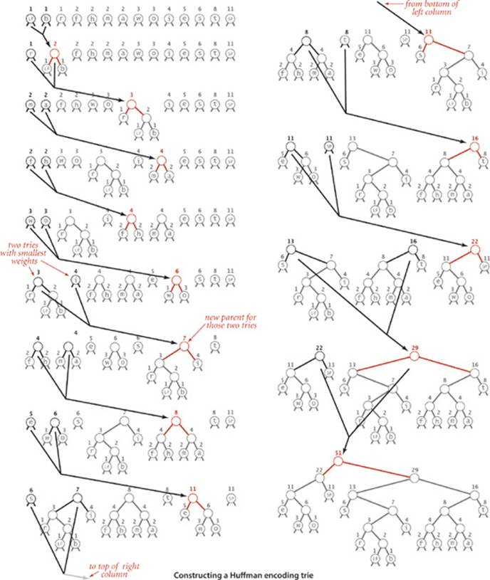
Trie construction
For reference as we describe the process, the figure on the facing page illustrates the process of constructing a Huffman trie for the input
it was the best of times it was the worst of times
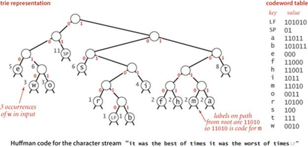
We keep the characters to be encoded in leaves and maintain the freq instance variable in each node that represents the frequency of occurrence of all characters in the subtree rooted at that node. The first step is to create a forest of 1-node trees (leaves), one for each character in the input stream, each assigned a freq value equal to its frequency of occurrence in the input. In the example, the input has 8 ts, 5 es, 11 spaces, and so forth. (Important note: To obtain these frequencies, we need to read the whole input stream—Huffman encoding is a two-pass algorithm because we will need to read the input stream a second time to compress it.) Next, we build the coding trie from the bottom up according to the frequencies. When building the trie, we view it as a binary trie with frequencies stored in the nodes; after it has been built, we view it as a trie for coding, as just described. The process works as follows: we find the two nodes with the smallest frequencies and then create a new node with those two nodes as children (and with frequency value set to the sum of the values of the children). This operation reduces the number of tries in the forest by one. Then we iterate the process: find the two nodes with smallest frequency in that forest and a create a new node created in the same way. Implementing the process is straightforward with a priority queue, as shown in the buildTrie() method at the bottom of this page. (For clarity, the tries in the figure are kept in sorted order.) Continuing, we build up larger and larger tries and at the same time reduce the number of tries in the forest by one at each step (remove two, add one). Ultimately, all the nodes are combined together into a single trie. The leaves in this trie have the characters to be encoded and their frequencies in the input; each non-leaf node is the sum of the frequencies of its two children. Nodes with low frequencies end up far down in the trie, and nodes with high frequencies end up near the root of the trie. The frequency in the root equals the number of characters in the input. Since it is a binary trie with characters only in its leaves, it defines a prefix-free code for the characters. Using the codeword table created by buildCode() for this example (shown at right in the diagram at the top of this page), we get the output bitstring which is 176 bits, a savings of 57 percent over the 408 bits needed to encode the 51 characters in standard 8-bit ASCII (not counting the cost of including the code, which we will soon consider). Moreover, since it is a Huffman code, no other prefix-free code can encode the input with fewer bits.
10111110100101101110001111110010000110101100-
01001110100111100001111101111010000100011011-
11101001011011100011111100100001001000111010-
01001110100111100001111101111010000100101010.
Building a Huffman encoding trie
private static Node buildTrie(int[] freq)
{
// Initialize priority queue with singleton trees.
MinPQ<Node> pq = new MinPQ<Node>();
for (char c = 0; c < R; c++)
if (freq[c] > 0)
pq.insert(new Node(c, freq[c], null, null));
while (pq.size() > 1)
{ // Merge two smallest trees.
Node x = pq.delMin();
Node y = pq.delMin();
Node parent = new Node('\0', x.freq + y.freq, x, y);
pq.insert(parent);
}
return pq.delMin();
}
Optimality
We have observed that high-frequency characters are nearer the root of the trie than lower-frequency characters and are therefore encoded with fewer bits, so this is a good code, but why is it an optimal prefix-free code? To answer this question, we begin by defining the weighted external path length of a tree to be the sum of the weight (associated frequency count) times depth (see page 226) of all of the leaves.
Proposition T. For any prefix-free code, the length of the encoded bitstring is equal to the weighted external path length of the corresponding trie.
Proof: The depth of each leaf is the number of bits used to encode the character in the leaf. Thus, the weighted external path length is the length of encoded bitstring: it is equivalent to the sum over all letters of the number of occurrences times the number of bits per occurrence.
For our example, there is one leaf at distance 2 (SP, with frequency 11), three leaves at distance 3 (e, s, and t, with total frequency 19), three leaves at distance 4 (w, o, and i, with total frequency 10), five leaves at distance 5 (r, f, h, m, and a, with total frequency 9) and two leaves at distance 6 (LFand b, with total frequency 2), so the sum total is 2·11 + 3·19 + 4·10 + 5·9 + 6·2 = 176, the length of the output bitstring, as expected.
Proposition U. Given a set of r symbols and frequencies, the Huffman algorithm builds an optimal prefix-free code.
Proof: By induction on r. Assume that the Huffman code is optimal for any set of fewer than r symbols. Let TH be the code computed by Huffman for the set of symbols and associated frequencies (s1, f1), . . ., (sr, fr) and denote the length of the code (weighted external path length of the trie) by W(TH). Suppose that (si, fi) and (sj, fj) are the first two symbols chosen. The algorithm then computes the code TH* for the set of r−1 symbols with (si, fi) and (si, fj) replaced by (s*, fi + fj) where s* is a new symbol in a leaf at some depth d. Note that
W(TH) = W(TH*) − d(fi + fj) + (d + 1)(fi + fj) = W(TH*) + (fi + fj)
Now consider an optimal trie T for (s1, f1), . . ., (sr, fr), of height h. Note that (si, fi) and (sj, fj) must be at depth h (else we could make a trie with lower external path length by swapping them with nodes at depth h). Also, assume (si, fi) and (sj, fj) are siblings by swapping (sj, fj) with (si, fi)’s sibling. Now consider the tree T* obtained by replacing their parent with (s*, fi + fj). Note that (by the same argument as above) W(T) = W(T*) + (fi + fj).
By the inductive hypothesis TH* is optimal: W(TH*) ≤ W(T*). Therefore,
W(TH) = W(TH*) + (fi + fj) ≤ W(T*) + (fi + fj) = W(T)
Since T is optimal, equality must hold, and TH is optimal.
Whenever a node is to be picked, it can be the case that there are several nodes with the same weight. Huffman’s method does not specify how such ties are to be broken. It also does not specify the left/right positions of the children. Different choices lead to different Huffman codes, but all such codes will encode the message with the optimal number of bits among prefix-free codes.
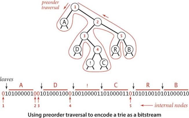
Writing and reading the trie
As we have emphasized, the savings figure quoted above is not entirely accurate, because the compressed bitstream cannot be decoded without the trie, so we must account for the cost of including the trie in the compressed output, along with the bitstring. For long inputs, this cost is relatively small, but in order for us to have a full data-compression scheme, we must write the trie onto a bitstream when compressing and read it back when expanding. How can we encode a trie as a bitstream, and then expand it? Remarkably, both tasks can be achieved with simple recursive procedures, based on a preorder traversal of the trie. The procedure writeTrie() below traverses a trie in preorder: when it visits an internal node, it writes a single 0 bit; when it visits a leaf, it writes a 1 bit, followed by the 8-bit ASCII code of the character in the leaf. The bitstring encoding of the Huffman trie for our ABRACADABRA! example is shown above. The first bit is 0, corresponding to the root; since the leaf containing A is encountered next, the next bit is 1, followed by 01000001, the 8-bit ASCII code for A; the next two bits are 0 because two internal nodes are encountered next, and so forth. The corresponding method readTrie() on the next page 835 reconstructs the trie from the bitstring: it reads a single bit to learn which type of node comes next: if a leaf (the bit is 1) it reads the next character and creates a leaf; if an internal node (the bit is 0) it creates an internal node and then (recursively) builds its left and right subtrees. Be sure that you understand these methods: their simplicity is somewhat deceiving.
Writing a trie as a bitstring
private static void writeTrie(Node x)
{ // Write bitstring-encoded trie.
if (x.isLeaf())
{
BinaryStdOut.write(true);
BinaryStdOut.write(x.ch, 8);
return;
}
BinaryStdOut.write(false);
writeTrie(x.left);
writeTrie(x.right);
}
Reconstructing a trie from the preorder bitstring representation
private static Node readTrie()
{
if (BinaryStdIn.readBoolean())
return new Node(BinaryStdIn.readChar(), 0, null, null);
return new Node('\0', 0, readTrie(), readTrie());
}
Huffman compression implementation
Along with the methods buildCode(), buildTrie(), readTrie() and writeTrie() that we have just considered (and the expand() method that we considered first), ALGORITHM 5.10 is a complete implementation of Huffman compression. To expand the overview that we considered several pages earlier, we view the bitstream to be encoded as a stream of 8-bit char values and compress it as follows:
• Read the input.
• Tabulate the frequency of occurrence of each char value in the input.
• Build the Huffman encoding trie corresponding to those frequencies.
• Build the corresponding codeword table, to associate a bitstring with each char value in the input.
• Write the trie, encoded as a bitstring.
• Write the count of characters in the input, encoded as a bitstring.
• Use the codeword table to write the codeword for each input character.
To expand a bitstream encoded in this way, we
• Read the trie (encoded at the beginning of the bitstream)
• Read the count of characters to be decoded
• Use the trie to decode the bitstream
With four recursive trie-processing methods and a seven-step compression process, Huffman compression is one of the more involved algorithms that we have considered, but it is also one of the most widely-used, because of its effectiveness.
Algorithm 5.10 Huffman compression
public class Huffman
{
private static int R = 256; // ASCII alphabet
// See page 828 for inner Node class.
// See text for helper methods and expand().
public static void compress()
{
// Read input.
String s = BinaryStdIn.readString();
char[] input = s.toCharArray();
// Tabulate frequency counts.
int[] freq = new int[R];
for (int i = 0; i < input.length; i++)
freq[input[i]]++;
// Build Huffman code trie.
Node root = buildTrie(freq);
// Build code table (recursive).
String[] st = new String[R];
buildCode(st, root, "");
// Print trie for decoder (recursive).
writeTrie(root);
// Print number of chars.
BinaryStdOut.write(input.length);
// Use Huffman code to encode input.
for (int i = 0; i < input.length; i++)
{
String code = st[input[i]];
for (int j = 0; j < code.length(); j++)
if (code.charAt(j) == '1')
BinaryStdOut.write(true);
else BinaryStdOut.write(false);
}
BinaryStdOut.close();
}
}
This implementation of Huffman encoding builds an explicit coding trie, using various helper methods that are presented and explained in the last several pages of text.
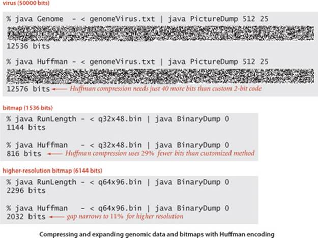
ONE REASON FOR THE POPULARITY of Huffman compression is that it is effective for various types of files, not just natural language text. We have been careful to code the method so that it can work properly for any 8-bit value in each 8-bit character. In other words, we can apply it to any bytestream whatsoever. Several examples, for file types that we have considered earlier in this section, are shown in the figure at the bottom of this page. These examples show that Huffman compression is competitive with both fixed-length encoding and run-length encoding, even though those methods are designed to perform well for certain types of files. Understanding the reason Huffman encoding performs well in these domains is instructive. In the case of genomic data, Huffman compression essentially discovers a 2-bit code, as the four letters appear with approximately equal frequency so that the Huffman trie is balanced, with each character assigned a 2-bit code. In the case of run-length encoding, 00000000 and 11111111 are likely to be the most frequently occurring characters, so they are likely to be encoded with 2 or 3 bits, leading to substantial compression.
A remarkable alternative to Huffman compression that was developed in the late 1970s and the early 1980s by A. Lempel, J. Ziv, and T. Welch has emerged as one of the most widely used compression methods because it is easy to implement and works well for a variety of file types.
The basic plan complements the basic plan for Huffman coding. Rather than maintain a table of variable-length codewords for fixed-length patterns in the input, we maintain a table of fixed-length codewords for variable-length patterns in the input. A surprising added feature of the method is that, by contrast with Huffman encoding, we do not have to encode the table.
LZW compression
To fix ideas, we will consider a compression example where we read the input as a stream of 7-bit ASCII characters and write the output as a stream of 8-bit bytes. (In practice, we typically use larger values for these parameters—our implementations use 8-bit inputs and 12-bit outputs.) We refer to input bytes as characters, sequences of input bytes as strings, and output bytes as codewords, even though these terms have slightly different meanings in other contexts. The LZW compression algorithm is based on maintaining a symbol table that associates string keys with (fixed-length) codeword values. We initialize the symbol table with the 128 possible single-character string keys and associate them with 8-bit codewords obtained by prepending 0 to the 7-bit value defining each character. For economy and clarity, we use hexadecimal to refer to codeword values, so 41 is the codeword for ASCII A, 52 for R, and so forth. We reserve the codeword 80 to signify end of file (EOF). We will assign the rest of the codeword values (81 through FF) to various substrings of the input that we encounter, by starting at 81 and incrementing the value for each new key added. To compress, we perform the following steps as long as there are unscanned input characters:
• Find the longest string s in the symbol table that is a prefix of the unscanned input.
• Write the 8-bit value (codeword) associated with s.
• Scan one character past s in the input.
• Associate the next codeword value with s + c (c appended to s) in the symbol table, where c is the next character in the input.
In the last of these steps, we look ahead to see the next character in the input to build the next dictionary entry, so we refer to that character c as the lookahead character. For the moment, we simply stop adding entries to the symbol table when we run out of codeword values (after assigning the value FF to some string)—we will later discuss alternate strategies.
LZW compression example
The figure below gives details of the operation of LZW compression for the example input ABRACADABRABRABRA. For the first seven characters, the longest prefix match is just one character, so we output the codeword associated with the character and associate the codewords from 81 through 87 to two-character strings. Then we find prefix matches with AB (so we output 81 and add ABR to the table), RA (so we output 83 and add RAB to the table), BR (so we output 82 and add BRA to the table), and ABR (so we output 88 and add ABRA to the table), leaving the last A (so we output its codeword, 41).
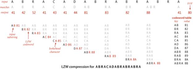
The input is 17 ASCII characters of 7 bits each for a total of 119 bits; the output is 13 codewords (including EOF) of 8 bits each for a total of 104 bits—a compression ratio of 87 percent even for this tiny example.
LZW trie representation
LZW compression involves two symbol-table operations:
• Find a longest-prefix match of the input with a symbol-table key.
• Add an entry associating the next codeword with the key formed by appending the lookahead character to that key.
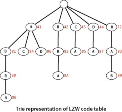
Our trie data structures of SECTION 5.2 are tailor-made for these operations. The trie representation for our example is shown at right. To find a longest prefix match, we traverse the trie from the root, matching node labels with input characters; to add a new codeword, we connect a new node labeled with the next codeword and the lookahead character to the node where the search terminated. In practice, we use a TST for space efficiency, as described in SECTION 5.2. The contrast with the use of tries in Huffman encoding is worth noting: for Huffman encoding, tries are useful because no prefix of a codeword is also a codeword; for LZW tries are useful because every prefix of an input-substring key is also a key.
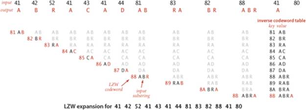
LZW expansion
The input for LZW expansion in our example is a sequence of 8-bit codewords; the output is a string of 7-bit ASCII characters. To implement expansion, we maintain a symbol table that associates strings of characters with codeword values (the inverse of the table used for compression). We fill the table entries from 00 to 7F with one-character strings, one for each ASCII character, set the first unassigned codeword value to 81 (reserving 80 for end of file), set the current string val to the one-character string consisting of the first character, and perform the following steps until reading codeword 80 (end of file):
• Write the current string val.
• Read a codeword x from the input.
• Set s to the value associated with x in the symbol table.
• Associate the next unasssigned codeword value to val + c in the symbol table, where c is the first character of s.
• Set the current string val to s.
This process is more complicated than compression because of the lookahead character: we need to read the next codeword to get the first character in the string associated with it, which puts the process one step out of synch. For the first seven codewords, we just look up and write the appropriate character, then look ahead one character and add a two-character entry to the symbol table, as before. Then we read 81 (so we write AB and add ABR to the table), 83 (so we write RA and add RAB to the table), 82 (so we write BR and add BRA to the table), and 88 (so we write ABR and add ABRA to the table), leaving 41. Finally we read the end-of-file character 80 (so we write A). At the end of the process, we have written the original input, as expected, and also built the same code table as for compression, but with the key-value roles inverted. Note that we can use a simple array-of-strings representation for the table, indexed by codeword.
Algorithm 5.11 LZW compression
public class LZW
{
private static final int R = 256; // number of input chars
private static final int L = 4096; // number of codewords = 2^12
private static final int W = 12; // codeword width
public static void compress()
{
String input = BinaryStdIn.readString();
TST<Integer> st = new TST<Integer>();
for (int i = 0; i < R; i++)
st.put("" + (char) i, i);
int code = R+1; // R is codeword for EOF.
while (input.length() > 0)
{
String s = st.longestPrefixOf(input); // Find max prefix match.
BinaryStdOut.write(st.get(s), W); // Print s's encoding.
int t = s.length();
if (t < input.length() && code < L) // Add s to symbol table.
st.put(input.substring(0, t + 1), code++);
input = input.substring(t); // Scan past s in input.
}
BinaryStdOut.write(R, W); // Write EOF.
BinaryStdOut.close();
}
public static void expand()
// See page 844.
}
This implementation of Lempel-Ziv-Welch data compression uses 8-bit input bytes and 12-bit codewords and is appropriate for arbitrary large files. Its codewords for the small example are similar to those discussed in the text: the single-character codewords have a leading 0; the others start at 100. Efficiency of this code depends on a constant-time substring() method (see page 202).
% more abraLZW.txt
ABRACADABRABRABRA
% java LZW - < abraLZW.txt | java HexDump 20
04 10 42 05 20 41 04 30 41 04 41 01 10 31 02 10 80 41 10 00
160 bits
Tricky situation
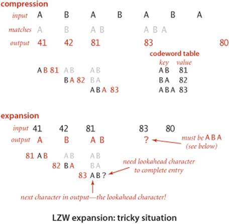
There is a subtle bug in the process just described, one that is often discovered by students (and experienced programmers!) only after developing an implementation based on the description above. The problem, illustrated in the example at right, is that it is possible for the lookahead process to get one character ahead of itself. In the example, the input string
ABABABA
is compressed to five output codewords
41 42 81 83 80
as shown in the top part of the figure. To expand, we read the codeword 41, output A, read the codeword 42 to get the lookahead character, add AB as table entry 81, output the B associated with 42, read the codeword 81 to get the lookahead character, add BA as table entry 82, and output the ABassociated with 81. So far, so good. But when we read the codeword 83 to get the lookahead character, we are stuck, because the reason that we are reading that codeword is to complete table entry 83! Fortunately, it is easy to test for that condition (it happens precisely when the codeword is the same as the table entry to be completed) and to correct it (the lookahead character must be the first character in that table entry, since that will be the next character to be output). In this example, this logic tells us that the lookahead character must be A (the first character in ABA). Thus, both the next output string and table entry 83 should be ABA.
Implementation
With these descriptions, implementing LZW encoding is straightforward, given in ALGORITHM 5.11 on the facing page (the implementation of expand() is on the next page). These implementations take 8-bit bytes as input (so we can compress any file, not just strings) and produce 12-bit codewords as output (so that we can get better compression by having a much larger dictionary). These values are specified in the (final) instance variables R, L, and W in the code. We use a TST (see SECTION 5.2) for the code table in compress() (taking advantage of the ability of trie data structures to support efficient implementations of longestPrefixOf()) and an array of strings for the inverse code table in expand(). With these choices, the code for compress() and expand() is little more than a line-by-line translation of the descriptions in the text. These methods are very effective as they stand. For certain files, they can be further improved by emptying the codeword table and starting over each time all the codeword values are used. These improvements, along with experiments to evaluate their effectiveness, are addressed in the exercises at the end of this section.
Algorithm 5.11 LZW expansion
public static void expand()
{
String[] st = new String[L];
int i; // next available codeword value
for (i = 0; i < R; i++) // Initialize table for chars.
st[i] = "" + (char) i;
st[i++] = " "; // (unused) lookahead for EOF
int codeword = BinaryStdIn.readInt(W);
String val = st[codeword];
while (true)
{
BinaryStdOut.write(val); // Write current substring.
codeword = BinaryStdIn.readInt(W);
if (codeword == R) break;
String s = st[codeword]; // Get next codeword.
if (i == codeword) // If lookahead is invalid,
s = val + val.charAt(0); // make codeword from last one.
if (i < L)
st[i++] = val + s.charAt(0); // Add new entry to code table.
val = s; // Update current codeword.
}
BinaryStdOut.close();
}
This implementation of expansion for the Lempel-Ziv-Welch algorithm is a bit more complicated than compression because of the need to extract the lookahead character from the next codeword and because of a tricky situation where lookahead is invalid (see text).
% java LZW - < abraLZW.txt | java LZW +
ABRACADABRABRABRA
% more ababLZW.txt
ABABABA
% java LZW - < ababLZW.txt | java LZW +
ABABABA
AS USUAL, it is worth your while to study carefully the examples given with the programs and at the bottom of this page of LZW compression in action. Over the several decades since its invention, it has proven to be a versatile and effective data-compression method.
Q&A
Q. Why BinaryStdIn and BinaryStdOut?
A. It’s a tradeoff between efficiency and convenience. StdIn can handle 8 bits at a time; BinaryStdIn has to handle each bit. Most applications are bytestream-oriented; data compression is a special case.
Q. Why close() ?
A. This requirement stems from the fact that standard output is actually a bytestream, so BinaryStdOut needs to know when to write the last byte.
Q. Can we mix StdIn and BinaryStdIn ?
A. That is not a good idea. Because of system and implementation dependencies, there is no guarantee of what might happen. Our implementations will raise an exception. On the other hand, there is no problem with mixing StdOut and BinaryStdOut (we do it in our code).
Q. Why is the Node class static in Huffman?
A. Our data-compression algorithms are organized as collections of static methods, not data-type implementations.
Q. Can I at least guarantee that my compression algorithm will not increase the length of a bitstream?
A. You can just copy it from input to output, but you still need to signify not to use a standard compression scheme. Commercial implementations sometimes make this guarantee, but it is quite weak and far from universal compression. Indeed, typical compression algorithms do not even make it past the second step of our first proof of PROPOSITION S: few algorithms will further compress a bitstring produced by that same algorithm.
Exercises
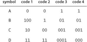
5.5.1 Consider the four variable-length codes shown in the table at right. Which of the codes are prefix-free? Uniquely decodable? For those that are uniquely decodable, give the decoding of 1000000000000.
5.5.2 Give an example of a uniquely decodable code that is not prefix-free.
Answer: Any suffix-free code is uniquely decodable.
5.5.3 Give an example of a uniquely decodable code that is not prefix free or suffix free.
Answer: {0011, 011, 11, 1110} or {01, 10, 011, 110}
5.5.4 Are {1, 100000, 00} and {01, 1001, 1011, 111, 1110} uniquely decodable? If not, find a string with two encodings.
5.5.5 Use RunLength on the file q128x192.bin from the booksite. How many bits are there in the compressed file?
5.5.6 How many bits are needed to encode N copies of the symbol a (as a function of N)? N copies of the sequence abc?
5.5.7 Give the result of encoding the strings a, aa, aaa, aaaa, ... (strings consisting of N a’s) with run-length, Huffman, and LZW encoding. What is the compression ratio as a function of N?
5.5.8 Give the result of encoding the strings ab, abab, ababab, abababab, ... (strings consisting of N repetitions of ab) with run-length, Huffman, and LZW encoding. What is the compression ratio as a function of N?
5.5.9 Estimate the compression ratio achieved by run-length, Huffman, and LZW encoding for a random ASCII string of length N (all characters equally likely at each position, independently).
5.5.10 In the style of the figure in the text, show the Huffman coding tree construction process when you use Huffman for the string "it was the age of foolishness". How many bits does the compressed bitstream require?
5.5.11 What is the Huffman code for a string whose characters are all from a two-character alphabet? Give an example showing the maximum number of bits that could be used in a Huffman code for an N-character string whose characters are all from a two-character alphabet.
5.5.12 Suppose that all of the symbol probabilities are negative powers of 2. Describe the Huffman code.
5.5.13 Suppose that all of the symbol frequencies are equal. Describe the Huffman code.
5.5.14 Suppose that the frequencies of the occurrence of all the characters to be encoded are different. Is the Huffman encoding tree unique?
5.5.15 Huffman coding could be extended in a straightforward way to encode in 2-bit characters (using 4-way trees). What would be the main advantage and the main disadvantage of doing so?
5.5.16 What is the LZW encoding of the following inputs?
a. T O B E O R N O T T O B E
b. Y A B B A D A B B A D A B B A D O O
c. A A A A A A A A A A A A A A A A A A A A A
5.5.17 Characterize the tricky situation in LZW coding.
Solution: Whenever it encounters cScSc, where c is a symbol and S is a string, cS is in the dictionary already but cSc is not.
5.5.18 Let Fk be the kth Fibonacci number. Consider N symbols, where the kth symbol has frequency Fk. Note that F1 + F1 + ... + FN = FN+2 − 1. Describe the Huffman code. Hint: The longest codeword has length N − 1.
5.5.19 Show that there are at least 2N−1 different Huffman codes corresponding to a given set of N symbols.
5.5.20 Give a Huffman code where the frequency of 0s in the output is much, much higher than the frequency of 1s.
5.5.21 Prove that the two longest codewords in a Huffman code have the same length.
5.5.22 Prove the following fact about Huffman codes: If the frequency of symbol i is strictly larger than the frequency of symbol j, then the length of the codeword for symbol i is less than or equal to the length of the codeword for symbol j.
5.5.23 What would be the result of breaking up a Huffman-encoded string into five-bit characters and Huffman-encoding that string?
5.5.24 In the style of the figures in the text, show the encoding trie and the compression and expansion processes when LZW is used for the string
it was the best of times it was the worst of times
Creative Problems
5.5.25 Fixed-length width code. Implement a class RLE that uses fixed-length encoding, to compress ASCII bytestreams using relatively few different characters, including the code as part of the encoded bitstream. Add code to compress() to make a string alpha with all the distinct characters in the message and use it to make an Alphabet for use in compress(), prepend alpha (8-bit encoding plus its length) to the compressed bitstream, then add code to expand() to read the alphabet before expansion.
5.5.26 Rebuilding the LZW dictionary. Modify LZW to empty the dictionary and start over when it is full. This approach is recommended in some applications because it better adapts to changes in the general character of the input.
5.5.27 Long repeats. Estimate the compression ratio achieved by run-length, Huffman, and LZW encoding for a string of length 2N formed by concatenating two copies of a random ASCII string of length N (see EXERCISE 5.5.9), under any assumptions that you think are reasonable.
All materials on the site are licensed Creative Commons Attribution-Sharealike 3.0 Unported CC BY-SA 3.0 & GNU Free Documentation License (GFDL)
If you are the copyright holder of any material contained on our site and intend to remove it, please contact our site administrator for approval.
© 2016-2026 All site design rights belong to S.Y.A.