Practical Data Science with R (2014)

Part 2. Modeling methods

In part 1, we discussed the initial stages of a data science project. After you’ve defined more precisely the questions you want to answer and the scope of the problem you want to solve, it’s time to analyze the data and find the answers. In part 2, we work with powerful modeling methods from statistics and machine learning.

Chapter 5 covers how to identify appropriate modeling methods to address your specific business problem. It also discusses how to evaluate the quality and effectiveness of models that you or others have discovered. The remaining chapters in part 2 cover specific modeling techniques.

Chapter 6 covers what we call memorization-based techniques. These methods make predictions based primarily on summary statistics of your data. We cover lookup tables, nearest-neighbor methods, Naive Bayes classification, and decision trees. Chapter 7 covers methods that fit simple functions with additive functional structure: linear and logistic regression. These two methods not only make predictions, but also provide you with information about the relationship between the input variables and the outcome.

Chapter 8 covers unsupervised methods: clustering and association rule mining. Unsupervised methods don’t make explicit outcome predictions; they discover relationships and hidden structure in the data. Chapter 9 touches on some more advanced modeling algorithms. We discuss bagged decision trees and random forests, generalized additive models, kernels, and support vector machines.

We work through every method that we cover with a specific data science problem, and a nontrivial dataset. In each chapter, we also discuss additional model evaluation procedures that are specific to the methods that we cover.

On completing part 2, you’ll be familiar with the most popular modeling methods, and you’ll have a sense of which methods are most appropriate for answering different types of questions.

Chapter 5. Choosing and evaluating models

This chapter covers

· Mapping business problems to machine learning tasks

· Evaluating model quality

· Validating model soundness

As a data scientist, your ultimate goal is to solve a concrete business problem: increase look-to-buy ratio, identify fraudulent transactions, predict and manage the losses of a loan portfolio, and so on. Many different statistical modeling methods can be used to solve any given problem. Each statistical method will have its advantages and disadvantages for a given business goal and business constraints. This chapter presents an outline of the most common machine learning and statistical methods used in data science.

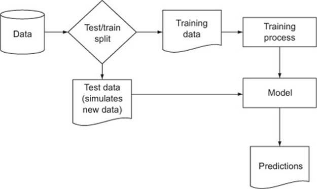
To make progress, you must be able to measure model quality during training and also ensure that your model will work as well in the production environment as it did on your training data. In general, we’ll call these two tasks model evaluation and model validation. To prepare for these statistical tests, we always split our data into training data and test data, as illustrated in figure 5.1.

Figure 5.1. Schematic model construction and evaluation

We define model evaluation as quantifying the performance of a model. To do this we must find a measure of model performance that’s appropriate to both the original business goal and the chosen modeling technique. For example, if we’re predicting who would default on loans, we have a classification task, and measures like precision and recall are appropriate. If we instead are predicting revenue lost to defaulting loans, we have a scoring task, and measures like root mean square error (RMSE) are appropriate. The point is this: there are a number of measures the data scientist should be familiar with.

We define model validation as the generation of an assurance that the model will work in production as well as it worked during training. It is a disaster to build a model that works great on the original training data and then performs poorly when used in production. The biggest cause of model validation failures is not having enough training data to represent the variety of what may later be encountered in production. For example, training a loan default model only on people who repaid their loans might score well on a simple evaluation (“predicts no defaults and is 100% accurate!”) but would obviously not be a good model to put into production. Validation techniques attempt to quantify this type of risk before you put a model into production.

5.1. Mapping problems to machine learning tasks

Your task is to map a business problem to a good machine learning method. To use a real-world situation, let’s suppose that you’re a data scientist at an online retail company. There are a number of business problems that your team might be called on to address:

· Predicting what customers might buy, based on past transactions

· Identifying fraudulent transactions

· Determining price elasticity (the rate at which a price increase will decrease sales, and vice versa) of various products or product classes

· Determining the best way to present product listings when a customer searches for an item

· Customer segmentation: grouping customers with similar purchasing behavior

· AdWord valuation: how much the company should spend to buy certain AdWords on search engines

· Evaluating marketing campaigns

· Organizing new products into a product catalog

Your intended uses of the model have a big influence on what methods you should use. If you want to know how small variations in input variables affect outcome, then you likely want to use a regression method. If you want to know what single variable drives most of a categorization, then decision trees might be a good choice. Also, each business problem suggests a statistical approach to try. If you’re trying to predict scores, some sort of regression is likely a good choice; if you’re trying to predict categories, then something like random forests is probably a good choice.

5.1.1. Solving classification problems

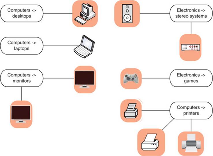
Suppose your task is to automate the assignment of new products to your company’s product categories, as shown in figure 5.2. This can be more complicated than it sounds. Products that come from different sources may have their own product classification that doesn’t coincide with the one that you use on your retail site, or they may come without any classification at all. Many large online retailers use teams of human taggers to hand-categorize their products. This is not only labor-intensive, but inconsistent and error-prone. Automation is an attractive option; it’s labor-saving, and can improve the quality of the retail site.

Figure 5.2. Assigning products to product categories

Product categorization based on product attributes and/or text descriptions of the product is an example of classification: deciding how to assign (known) labels to an object. Classification itself is an example of what is called supervised learning: in order to learn how to classify objects, you need a dataset of objects that have already been classified (called the training set). Building training data is the major expense for most classification tasks, especially text-related ones. Table 5.1 lists some of the more common effective classification methods.

Table 5.1. Some common classification methods

^a . Strictly speaking, logistic regression is scoring (covered in the next section). To turn a scoring algorithm into a classifier requires a threshold. For scores higher than the threshold, assign one label; for lower scores, assign an alternative label.

Multicategory vs. two-category classification

Product classification is an example of multicategory or multinomial classification. Most classification problems and most classification algorithms are specialized for two-category, or binomial, classification. There are tricks to using binary classifiers to solve multicategory problems (for example, building one classifier for each category, called a “one versus rest” classifier). But in most cases it’s worth the effort to find a suitable multiple-category implementation, as they tend to work better than multiple binary classifiers (for example, using the package mlogit instead of the base method glm() for logistic regression).

5.1.2. Solving scoring problems

For a scoring example, suppose that your task is to help evaluate how different marketing campaigns can increase valuable traffic to the website. The goal is not only to bring more people to the site, but to bring more people who buy. You’re looking at a number of different factors: the communication channel (ads on websites, YouTube videos, print media, email, and so on); the traffic source (Facebook, Google, radio stations, and so on); the demographic targeted; the time of year; and so on.

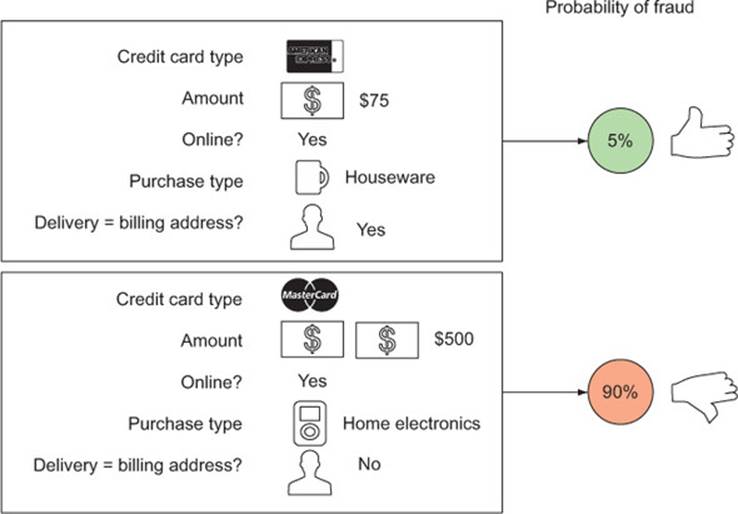
Predicting the increase in sales from a particular marketing campaign is an example of regression, or scoring. Fraud detection can be considered scoring, too, if you’re trying to estimate the probability that a given transaction is a fraudulent one (rather than just returning a yes/no answer). This is shown in figure 5.3. Scoring is also an instance of supervised learning.

Figure 5.3. Notional example of determining the probability that a transaction is fraudulent

Common scoring methods

We’ll cover the following two general scoring methods in more detail in later chapters.

Linear regression

Linear regression builds a model such that the predicted numerical output is a linear additive function of the inputs. This can be a very effective approximation, even when the underlying situation is in fact nonlinear. The resulting model also gives an indication of the relative impact of each input variable on the output. Linear regression is often a good first model to try when trying to predict a numeric value.

Logistic regression

Logistic regression always predicts a value between 0 and 1, making it suitable for predicting probabilities (when the observed outcome is a categorical value) and rates (when the observed outcome is a rate or ratio). As we mentioned, logistic regression is an appropriate approach to the fraud detection problem, if what you want to estimate is the probability that a given transaction is fraudulent or legitimate.

5.1.3. Working without known targets

The preceding methods require that you have a training dataset of situations with known outcomes. In some situations, there’s not (yet) a specific outcome that you want to predict. Instead, you may be looking for patterns and relationships in the data that will help you understand your customers or your business better.

These situations correspond to a class of approaches called unsupervised learning: rather than predicting outputs based on inputs, the objective of unsupervised learning is to discover similarities and relationships in the data. Some common clustering methods include these:

· K-means clustering

· Apriori algorithm for finding association rules

· Nearest neighbor

But these methods make more sense when we provide some context and explain their use, as we do next.

When to use basic clustering

Suppose you want to segment your customers into general categories of people with similar buying patterns. You might not know in advance what these groups should be.

This problem is a good candidate for k-means clustering. K-means clustering is one way to sort the data into groups such that members of a cluster are more similar to each other than they are to members of other clusters.

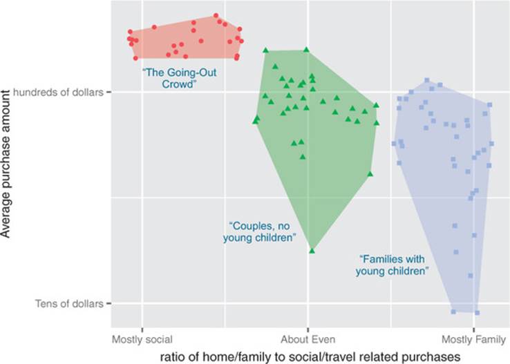
Suppose that you find (as in figure 5.4) that your customers cluster into those with young children, who make more family-oriented purchases, and those with no children or with adult children, who make more leisure- and social-activity-related purchases. Once you have assigned a customer into one of those clusters, you can make general statements about their behavior. For example, a customer in the with-young-children cluster is likely to respond more favorably to a promotion on attractive but durable glassware than to a promotion on fine crystal wine glasses.

Figure 5.4. Notional example of clustering your customers by purchase pattern and purchase amount

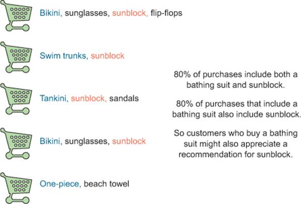
When to use association rules

You might be interested in directly determining which products tend to be purchased together. For example, you might find that bathing suits and sunglasses are frequently purchased at the same time, or that people who purchase certain cult movies, like Repo Man, will often buy the movie soundtrack at the same time.

This is a good application for association rules (or even recommendation systems). You can mine useful product recommendations: whenever you observe that someone has put a bathing suit into their shopping cart, you can recommend suntan lotion, as well. This is shown in figure 5.5. We’ll cover the Apriori algorithm for discovering association rules in section 8.2.

Figure 5.5. Notional example of finding purchase patterns in your data

When to use nearest neighbor methods

Another way to make product recommendations is to find similarities in people (figure 5.6). For example, to make a movie recommendation to customer JaneB, you might look for the three customers whose movie rental histories are the most like hers. Any movies that those three people rented, but JaneB has not, are potentially useful recommendations for her.

Figure 5.6. Look to the customers with similar movie-watching patterns as JaneB for her movie recommendations.

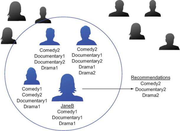
This can be solved with nearest neighbor (or k-nearest neighbor methods, with K = 3). Nearest neighbor algorithms predict something about a data point p (like a customer’s future purchases) based on the data point or points that are most similar to p. We’ll cover the nearest neighbor approach in section 6.3.3.

5.1.4. Problem-to-method mapping

Table 5.2 maps some typical business problems to their corresponding machine learning task, and to some typical algorithms to tackle each task.

Table 5.2. From problem to approach

Notice that some problems show up multiple times in the table. Our mapping isn’t hard-and-fast; any problem can be approached through a variety of mindsets, with a variety of algorithms. We’re merely listing some common mappings and approaches to typical business problems. Generally, these should be among the first approaches to consider for a given problem; if they don’t perform well, then you’ll want to research other approaches, or get creative with data representation and with variations of common algorithms.

Prediction vs. forecasting

In everyday language, we tend to use the terms prediction and forecasting interchangeably. Technically, to predict is to pick an outcome, such as “It will rain tomorrow,” and to forecast is to assign a probability: “There’s an 80% chance it will rain tomorrow.” For unbalanced class applications (such as predicting credit default), the difference is important. Consider the case of modeling loan defaults, and assume the overall default rate is 5%. Identifying a group that has a 30% default rate is an inaccurate prediction (you don’t know who in the group will default, and most people in the group won’t default), but potentially a very useful forecast (this group defaults at six times the overall rate).

5.2. Evaluating models

When building a model, the first thing to check is if the model even works on the data it was trained from. In this section, we do this by introducing quantitative measures of model performance. From an evaluation point of view, we group model types this way:

· Classification

· Scoring

· Probability estimation

· Ranking

· Clustering

For most model evaluations, we just want to compute one or two summary scores that tell us if the model is effective. To decide if a given score is high or low, we have to appeal to a few ideal models: a null model (which tells us what low performance looks like), a Bayes rate model (which tells us what high performance looks like), and the best single-variable model (which tells us what a simple model can achieve). We outline the concepts in table 5.3.

Table 5.3. Ideal models to calibrate against

^a There are a few machine learning magic methods that can introduce new synthetic features and in fact alter the Bayes rate. Typically, this is done by adding higher-order terms, interaction terms, or kernelizing.

In this section, we’ll present the standard measures of model quality, which are useful in model construction. In all cases, we suggest that in addition to the standard model quality assessments you try to design your own custom “business-oriented loss function” with your project sponsor or client. Usually this is as simple as assigning a notional dollar value to each outcome and then seeing how your model performs under that criterion. Let’s start with how to evaluate classification models and then continue from there.

5.2.1. Evaluating classification models

A classification model places examples into two or more categories. The most common measure of classifier quality is accuracy. For measuring classifier performance, we’ll first introduce the incredibly useful tool called the confusion matrix and show how it can be used to calculate many important evaluation scores. The first score we’ll discuss is accuracy, and then we’ll move on to better and more detailed measures such as precision and recall.

Let’s use the example of classifying email into spam (email we in no way want) and non-spam (email we want). A ready-to-go example (with a good description) is the Spambase dataset (http://mng.bz/e8Rh). Each row of this dataset is a set of features measured for a specific email and an additional column telling whether the mail was spam (unwanted) or non-spam (wanted). We’ll quickly build a spam classification model so we have results to evaluate. To do this, download the file Spambase/spamD.tsv from the book’s GitHub site (https://github.com/WinVector/zmPDSwR/tree/master/Spambase) and then perform the steps shown in the following listing.

Listing 5.1. Building and applying a logistic regression spam model

spamD <- read.table('spamD.tsv',header=T,sep='\t')

spamTrain <- subset(spamD,spamD$rgroup>=10)

spamTest <- subset(spamD,spamD$rgroup<10)

spamVars <- setdiff(colnames(spamD),list('rgroup','spam'))

spamFormula <- as.formula(paste('spam=="spam"',

paste(spamVars,collapse=' + '),sep=' ~ '))

spamModel <- glm(spamFormula,family=binomial(link='logit'),

data=spamTrain)

spamTrain$pred <- predict(spamModel,newdata=spamTrain,

type='response')

spamTest$pred <- predict(spamModel,newdata=spamTest,

type='response')

print(with(spamTest,table(y=spam,glmPred=pred>0.5)))

## glmPred

## y FALSE TRUE

## non-spam 264 14

## spam 22 158

A sample of the results of our simple spam classifier is shown in the next listing.

Listing 5.2. Spam classifications

> sample <- spamTest[c(7,35,224,327),c('spam','pred')]

> print(sample)

spam pred

115 spam 0.9903246227

361 spam 0.4800498077

2300 non-spam 0.0006846551

3428 non-spam 0.0001434345

The confusion matrix

The absolute most interesting summary of classifier performance is the confusion matrix. This matrix is just a table that summarizes the classifier’s predictions against the actual known data categories.

The confusion matrix is a table counting how often each combination of known outcomes (the truth) occurred in combination with each prediction type. For our email spam example, the confusion matrix is given by the following R command.

Listing 5.3. Spam confusion matrix

> cM <- table(truth=spamTest$spam,prediction=spamTest$pred>0.5)

> print(cM)

prediction

truth FALSE TRUE

non-spam 264 14

spam 22 158

Using this summary, we can now start to judge the performance of the model. In a two-by-two confusion matrix, every cell has a special name, as illustrated in table 5.4.

Table 5.4. Standard two-by-two confusion matrix

Changing a score to a classification

Note that we converted the numerical prediction score into a decision by checking if the score was above or below 0.5. For some scoring models (like logistic regression) the 0.5 score is likely a high accuracy value. However, accuracy isn’t always the end goal, and for unbalanced training data the 0.5 threshold won’t be good. Picking thresholds other than 0.5 can allow the data scientist to trade precision for recall (two terms that we’ll define later in this chapter). You can start at 0.5, but consider trying other thresholds and looking at the ROC curve.

Most of the performance measures of a classifier can be read off the entries of this confusion matrix. We start with the most common measure: accuracy.

Accuracy

Accuracy is by far the most widely known measure of classifier performance. For a classifier, accuracy is defined as the number of items categorized correctly divided by the total number of items. It’s simply what fraction of the time the classifier is correct. At the very least, you want a classifier to be accurate. In terms of our confusion matrix, accuracy is (TP+TN)/(TP+FP+TN+FN)=(cM[1,1]+cM[2,2])/sum(cM) or 92% accurate. The error of around 8% is unacceptably high for a spam filter, but good for illustrating different sorts of model evaluation criteria.

Categorization accuracy isn’t the same as numeric accuracy

It’s important to not confuse accuracy used in a classification sense with accuracy used in a numeric sense (as in ISO 5725, which defines score-based accuracy as a numeric quantity that can be decomposed into numeric versions of trueness and precision). These are, unfortunately, two different meanings of the word.

Before we move on, we’d like to share the confusion matrix of a good spam filter. In the next listing we create the confusion matrix for the Akismet comment spam filter from the Win-Vector blog.

Listing 5.4. Entering data by hand

> t <- as.table(matrix(data=c(288-1,17,1,13882-17),nrow=2,ncol=2))

> rownames(t) <- rownames(cM)

> colnames(t) <- colnames(cM)

> print(t)

FALSE TRUE

non-spam 287 1

spam 17 13865

Because the Akismet filter uses link destination clues and determination from other websites (in addition to text features), it achieves a more acceptable accuracy of (t[1,1]+t[2,2])/sum(t), or over 99.87%. More importantly, Akismet seems to have suppressed fewer good comments. Our next section on precision and recall will help quantify this distinction.

Accuracy is an inappropriate measure for unbalanced classes

Suppose we have a situation where we have a rare event (say, severe complications during childbirth). If the event we’re trying to predict is rare (say, around 1% of the population), the null model—the rare event never happens—is very accurate. The null model is in fact more accurate than a useful (but not perfect model) that identifies 5% of the population as being “at risk” and captures all of the bad events in the 5%. This is not any sort of paradox. It’s just that accuracy is not a good measure for events that have unbalanced distribution or unbalanced costs (different costs of “type 1” and “type 2” errors).

Precision and recall

Another evaluation measure used by machine learning researchers is a pair of numbers called precision and recall. These terms come from the field of information retrieval and are defined as follows. Precision is what fraction of the items the classifier flags as being in the class actually are in the class. So precision is TP/(TP+FP), which is cM[2,2]/(cM[2,2]+cM[1,2]), or about 0.92 (it is only a coincidence that this is so close to the accuracy number we reported earlier). Again, precision is how often a positive indication turns out to be correct. It’s important to remember that precision is a function of the combination of the classifier and the dataset. It doesn’t make sense to ask how precise a classifier is in isolation; it’s only sensible to ask how precise a classifier is for a given dataset.

In our email spam example, 93% precision means 7% of what was flagged as spam was in fact not spam. This is an unacceptable rate for losing possibly important messages. Akismet, on the other hand, had a precision of t[2,2]/(t[2,2]+t[1,2]), or over 99.99%, so in addition to having high accuracy, Akismet has even higher precision (very important in a spam filtering application).

The companion score to precision is recall. Recall is what fraction of the things that are in the class are detected by the classifier, or TP/(TP+FN)=cM[2,2]/(cM[2,2]+cM[2,1]). For our email spam example this is 88%, and for the Akismet example it is 99.87%. In both cases most spam is in fact tagged (we have high recall) and precision is emphasized over recall (which is appropriate for a spam filtering application).

It’s important to remember this: precision is a measure of confirmation (when the classifier indicates positive, how often it is in fact correct), and recall is a measure of utility (how much the classifier finds of what there actually is to find). Precision and recall tend to be relevant to business needs and are good measures to discuss with your project sponsor and client.

F1

The F1 score is a useful combination of precision and recall. If either precision or recall is very small, then F1 is also very small. F1 is defined as 2*precision*recall/(precision+recall). So our email spam example with 0.93 precision and 0.88 recall has an F1 score of 0.90. The idea is that a classifier that improves precision or recall by sacrificing a lot of the complementary measure will have a lower F1.

Sensitivity and specificity

Scientists and doctors tend to use a pair of measures called sensitivity and specificity.

Sensitivity is also called the true positive rate and is exactly equal to recall. Specificity is also called the true negative rate and is equal to TN/(TN+FP)=cM[1,1]/(cM[1,1] +cM[1,2]) or about 95%. Both sensitivity and specificity are measures of effect: what fraction of class members are identified as positive and what fraction of non-class members are identified as negative.

An important property of sensitivity and specificity is this: if you flip your labels (switch from spam being the class you’re trying to identify to non-spam being the class you’re trying to identify), you just switch sensitivity and specificity. Also, any of the so-called null classifiers (classifiers that always say positive or always say negative) always return a zero score on either sensitivity or specificity. So useless classifiers always score poorly on at least one of these measures. Finally, unlike precision and accuracy, sensitivity and specificity each only involve entries from a single row of table 5.4. So they’re independent of the population distribution (which means they’re good for some applications and poor for others).

Common classification performance measures

Table 5.5 summarizes the behavior of both the email spam example and the Akismet example under the common measures we’ve discussed.

Table 5.5. Example classifier performance measures

All of these formulas can seem confusing, and the best way to think about them is to shade in various cells in table 5.4. If your denominator cells shade in a column, then you’re measuring a confirmation of some sort (how often the classifier’s decision is correct). If your denominator cells shade in a row, then you’re measuring effectiveness (how much of a given class is detected by a the classifier). The main idea is to use these standard scores and then work with your client and sponsor to see what most models their business needs. For each score, you should ask them if they need that score to be high and then run a quick thought experiment with them to confirm you’ve gotten their business need. You should then be able to write a project goal in terms of a minimum bound on a pair of these measures. Table 5.6 shows a typical business need and an example follow-up question for each measure.

Table 5.6. Classifier performance measures business stories

One conclusion for this dialogue process on spam classification would be to recommend writing the business goals as maximizing sensitivity while maintaining a specificity of at least 0.999.

5.2.2. Evaluating scoring models

Evaluating models that assign scores can be a somewhat visual task. The main concept is looking at what is called the residuals or the difference between our predictions f(x[i,]) and actual outcomes y[i]. Figure 5.7 illustrates the concept.

Figure 5.7. Scoring residuals

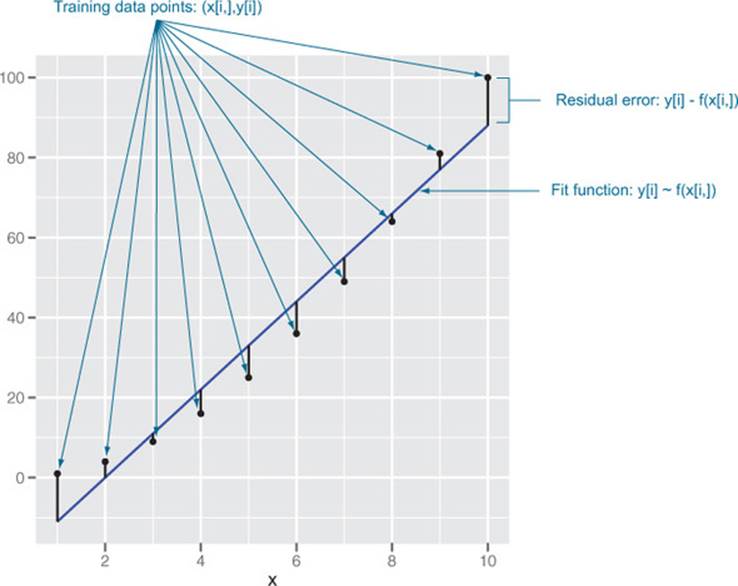
The data and graph in figure 5.7 were produced by the R commands in the following listing.

Listing 5.5. Plotting residuals

d <- data.frame(y=(1:10)^2,x=1:10)

model <- lm(y~x,data=d)

d$prediction <- predict(model,newdata=d)

library('ggplot2')

ggplot(data=d) + geom_point(aes(x=x,y=y)) +

geom_line(aes(x=x,y=prediction),color='blue') +

geom_segment(aes(x=x,y=prediction,yend=y,xend=x)) +

scale_y_continuous('')

Root mean square error

The most common goodness-of-fit measure is called root mean square error (RMSE). This is the square root of the average square of the difference between our prediction and actual values. Think of it as being like a standard deviation: how much your prediction is typically off. In our case, the RMSE is sqrt(mean((d$prediction-d$y)^2)), or about 7.27. The RMSE is in the same units as your y-values are, so if your y-units are pounds, your RMSE is in pounds. RMSE is a good measure, because it is often what the fitting algorithms you’re using are explicitly trying to minimize. A good RMSE business goal would be “We want the RMSE on account valuation to be under $1,000 per account.”

Most RMSE calculations (including ours) don’t include any bias correction for sample size or model complexity, though you’ll see adjusted RMSE in chapter 7.

R-squared

Another important measure of fit is called R-squared (or R², or the coefficient of determination). It’s defined as 1.0 minus how much unexplained variance your model leaves (measured relative to a null model of just using the average y as a prediction). In our case, the R-squared is 1-sum((d$prediction-d$y)^2)/sum((mean(d$y)-d$y)^2), or 0.95. R-squared is dimensionless (it’s not the units of what you’re trying to predict), and the best possible R-squared is 1.0 (with near-zero or negative R-squared being horrible). R-squared can be thought of as what fraction of the y variation is explained by the model. For linear regression (with appropriate bias corrections), this interpretation is fairly clear. Some other models (like logistic regression) use deviance to report an analogous quantity called pseudo R-squared.

Under certain circumstances, R-squared is equal to the square of another measure called the correlation (or Pearson product-moment correlation coefficient; see http://mng.bz/ndYf). R-squared can be derived from RMSE plus a few facts about the data (so R-squared can be thought of as a normalized version of RMSE). A good R-squared business goal would be “We want the model to explain 70% of account value.”

However, R-squared is not always the best business-oriented metric. For example, it’s hard to tell what a 10% reduction of RMSE would mean in relation to the Netflix Prize. But it would be easy to map the number of ranking errors and amount of suggestion diversity to actual Netflix business benefits.

Correlation

Correlation is very helpful in checking if variables are potentially useful in a model. Be advised that there are at least three calculations that go by the name of correlation: Pearson, Spearman, and Kendall (see help(cor)). The Pearson coefficient checks for linear relations, the Spearman coefficient checks for rank or ordered relations, and the Kendall coefficient checks for degree of voting agreement. Each of these coefficients performs a progressively more drastic transform than the one before and has well-known direct significance tests (see help(cor.test)).

Don’t use correlation to evaluate model quality in production

It’s tempting to use correlation to measure model quality, but we advise against it. The problem is this: correlation ignores shifts and scaling factors. So correlation is actually computing if there is any shift and rescaling of your predictor that is a good predictor. This isn’t a problem for training data (as these predictions tend to not have a systematic bias in shift or scaling by design) but can mask systematic errors that may arise when a model is used in production.

Absolute error

For many applications (especially those involving predicting monetary amounts), measures such as absolute error (sum(abs(d$prediction-d$y))), mean absolute error (sum(abs(d$prediction-d$y))/length(d$y)), and relative absolute error (sum(abs(d$prediction-d$y))/sum(abs(d$y))) are tempting measures. It does make sense to check and report these measures, but it’s usually not advisable to make these measures the project goal or to attempt to directly optimize them. This is because absolute error measures tend not to “get aggregates right” or “roll up reasonably” as most of the squared errors do.

As an example, consider an online advertising company with three advertisement purchases returning $0, $0, and $25 respectively. Suppose our modeling task is as simple as picking a single summary value not too far from the original three prices. The price minimizing absolute error is the median, which is $0, yielding an absolute error of sum(abs(c(0,0,25)-20)), or $25. The price minimizing square error is the mean, which is $8.33 (which has a worse absolute error of $33.33). However the median price of $0 misleadingly values the entire campaign at $0. One great advantage of the mean is this: aggregating a mean prediction gives an unbiased prediction of the aggregate in question. It is often an unstated project need that various totals or roll-ups of the predicted amounts be close to the roll-ups of the unknown values to be predicted. For monetary applications, predicting the totals or aggregates accurately is often more important than getting individual values right. In fact, most statistical modeling techniques are designed for regression, which is the unbiased prediction of means or expected values.

5.2.3. Evaluating probability models

Probability models are useful for both classification and scoring tasks. Probability models are models that both decide if an item is in a given class and return an estimated probability (or confidence) of the item being in the class. The modeling techniques of logistic regression and decision trees are fairly famous for being able to return good probability estimates. Such models can be evaluated on their final decisions, as we’ve already shown in section 5.2.1, but they can also be evaluated in terms of their estimated probabilities. We’ll continue the example from section 5.2.1 in this vein. In our opinion, most of the measures for probability models are very technical and very good at comparing the qualities of different models on the same dataset. But these criteria aren’t easy to precisely translate into businesses needs. So we recommend tracking them, but not using them with your project sponsor or client.

When thinking about probability models, it’s useful to construct a double density plot (illustrated in figure 5.8).

Figure 5.8. Distribution of score broken up by known classes

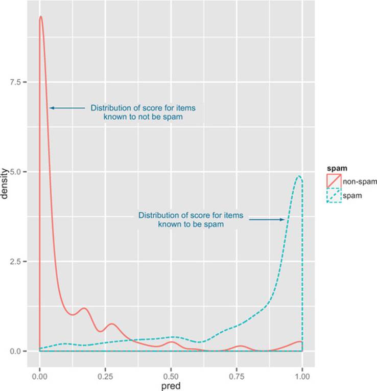
Listing 5.6. Making a double density plot

ggplot(data=spamTest) +

geom_density(aes(x=pred,color=spam,linetype=spam))

Figure 5.8 is particularly useful at picking and explaining classifier thresholds. It also illustrates what we’re going to try to check when evaluating estimated probability models: examples in the class should mostly have high scores and examples not in the class should mostly have low scores.

The receiver operating characteristic curve

The receiver operating characteristic curve (or ROC curve) is a popular alternative to the double density plot. For each different classifier we’d get by picking a different score threshold between positive and negative determination, we plot both the true positive rate and the false positive rate. This curve represents every possible trade-off between sensitivity and specificity that is available for this classifier. The steps to produced the ROC plot in figure 5.9 are shown in the next listing. In the last line, we compute the AUC or area under the curve, which is 1.0 for perfect classifiers and 0.5 for classifiers that do no better than random guesses.

Figure 5.9. ROC curve for the email spam example

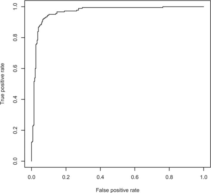
Listing 5.7. Plotting the receiver operating characteristic curve

library('ROCR')

eval <- prediction(spamTest$pred,spamTest$spam)

plot(performance(eval,"tpr","fpr"))

print(attributes(performance(eval,'auc'))$y.values[[1]])

[1] 0.9660072

We’re not big fans of the AUC; many of its claimed interpretations are either incorrect (see http://mng.bz/Zugx) or not relevant to actual business questions.^[1] But working around the ROC curve with your project client is a good way to explore possible project goal trade-offs.

¹ See D. J. Hand, “Measuring classifier performance: a coherent alternative to the area under the ROC curve,” Machine Learning, 2009, 77(1), pp. 103-123.

Log likelihood

An important evaluation of an estimated probability is the log likelihood. The log likelihood is the logarithm of the product of the probability the model assigned to each example.^[2] For a spam email with an estimated likelihood of 0.9 of being spam, the log likelihood is log(0.9); for a non-spam email, the same score of 0.9 is a log likelihood of log(1-0.9) (or just the log of 0.1, which was the estimated probability of not being spam). The principle is this: if the model is a good explanation, then the data should look likely (not implausible) under the model. The following listing shows how the log likelihood of our example is derived.

² The traditional way of calculating the log likelihood is to compute the sum of the logarithms of the probabilities the model assigns to each example.

Listing 5.8. Calculating log likelihood

> sum(ifelse(spamTest$spam=='spam',

log(spamTest$pred),

log(1-spamTest$pred)))

[1] -134.9478

> sum(ifelse(spamTest$spam=='spam',

log(spamTest$pred),

log(1-spamTest$pred)))/dim(spamTest)[[1]]

[1] -0.2946458

The first term (-134.9478) is the model log likelihood the model assigns to the test data. This number will always be negative, and is better as we get closer to 0. The second expression is the log likelihood rescaled by the number of data points to give us a rough average surprise per data point. Now a good null model in this case would be always returning the probability of 180/458 (the number of known spam emails over the total number of emails as the best single-number estimate of the chance of spam). This null model gives the log likelihood shown in the next listing.

Listing 5.9. Computing the null model’s log likelihood

> pNull <- sum(ifelse(spamTest$spam=='spam',1,0))/dim(spamTest)[[1]]

> sum(ifelse(spamTest$spam=='spam',1,0))*log(pNull) +

sum(ifelse(spamTest$spam=='spam',0,1))*log(1-pNull)

[1] -306.8952

The spam model assigns a log likelihood of -134.9478, which is much better than the null model’s -306.8952.

Deviance

Another common measure when fitting probability models is the deviance. The deviance is defined as -2*(logLikelihood-S), where S is a technical constant called “the log likelihood of the saturated model.” The lower the residual deviance, the better the model. In most cases, the saturated model is a perfect model that returns probability 1 for items in the class and probability 0 for items not in the class (so S=0). We’re most concerned with differences of deviance, such as the difference between the null deviance and the model deviance (and in the case of our example, the Ss cancels out). In our case, this difference is -2*(-306.8952-S) - -2*(-134.9478-S)=344.9. With S=0 the deviance can be used to calculate a pseudo R-squared (see http://mng.bz/j338). Think of the null deviance as how much variation there is to explain, and the model deviance as how much was left unexplained by the model. So in this case, our pseudo R-squared is 1 - (-2*(-134.9478-S))/(-2*(-306.8952-S)) =0.56 (good, but not great).

AIC

An important variant of deviance is the Akaike information criterion (AIC). This is equivalent to deviance + 2*numberOfParameters used in the model used to make the prediction. Thus, AIC is deviance penalized for model complexity. A nice trick is to do as the Bayesians do: useBayesian information criterion (BIC) (instead of AIC) where an empirical estimate of the model complexity (such as 2*2^entropy, instead of 2*numberOfParameters) is used as the penalty. The AIC is useful for comparing models with different measures of complexity and variables with differing number of levels.^[3]

³ Rigorously balancing model quality and model complexity is a deep problem.

Entropy

Entropy is a fairly technical measure of information or surprise, and is measured in a unit called bits. If p is a vector containing the probability of each possible outcome, then the entropy of the outcomes is calculated as sum(-p*log(p,2)) (with the convention that 0*log(0) = 0). As entropy measures surprise, you want what’s called the conditional entropy of your model to be appreciably lower than the original entropy. The conditional entropy is a measure that gives an indication of how good the prediction is on different categories, tempered by how often it predicts different categories. In terms of our confusion matrix cM, we can calculate the original entropy and conditional (or residual) entropy as shown next.

Listing 5.10. Calculating entropy and conditional entropy

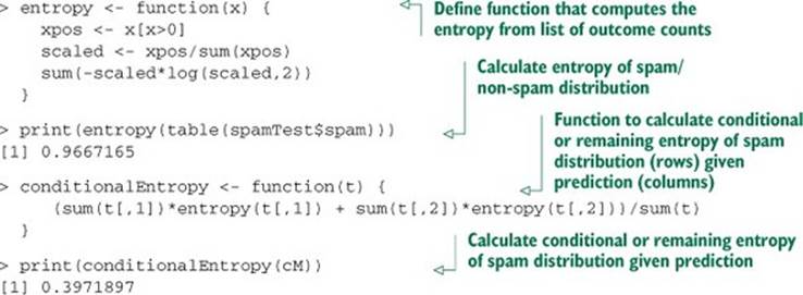
We see the initial entropy is 0.9667 bits per example (so a lot of surprise is present), and the conditional entropy is only 0.397 bits per example.

5.2.4. Evaluating ranking models

Ranking models are models that, given a set of examples, sort the rows or (equivalently) assign ranks to the rows. Ranking models are often trained by converting groups of examples into many pair-wise decisions (statements like “a is before b”). You can then apply the criteria for evaluating classifiers to quantify the quality of your ranking function. Two other standard measures of a ranking model are Spearman’s rank correlation coefficient (treating assigned rank as a numeric score) and the data mining concept of lift (treating ranking as sorting; see http://mng.bz/1LBl). Ranking evaluation is well handled by business-driven ad hoc methods, so we won’t spend any more time on this issue.

5.2.5. Evaluating clustering models

Clustering models are hard to evaluate because they’re unsupervised: the clusters that items are assigned to are generated by the modeling procedure, not supplied in a series of annotated examples. Evaluation is largely checking observable summaries about the clustering. As a quick example, we’ll demonstrate evaluating division of 100 random points in a plane into five clusters. We generate our example data and proposed k-means-based clustering in the next listing.

Listing 5.11. Clustering random data in the plane

set.seed(32297)

d <- data.frame(x=runif(100),y=runif(100))

clus <- kmeans(d,centers=5)

d$cluster <- clus$cluster

Because our example is two-dimensional, it’s easy to visualize, so we can use the following commands to generate figure 5.10, which we can refer to when thinking about clustering quality.

Figure 5.10. Clustering example

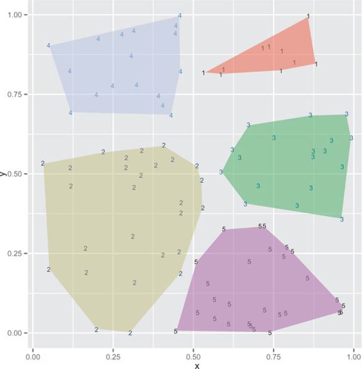
Listing 5.12. Plotting our clusters

library('ggplot2'); library('grDevices')

h <- do.call(rbind,

lapply(unique(clus$cluster),

function(c) { f <- subset(d,cluster==c); f[chull(f),]}))

ggplot() +

geom_text(data=d,aes(label=cluster,x=x,y=y,

color=cluster),size=3) +

geom_polygon(data=h,aes(x=x,y=y,group=cluster,fill=as.factor(cluster)),

alpha=0.4,linetype=0) +

theme(legend.position = "none")

The first qualitative metrics are how many clusters you have (sometimes chosen by the user, sometimes chosen by the algorithm) and the number of items in each cluster. This is quickly calculated by the table command.

Listing 5.13. Calculating the size of each cluster

> table(d$cluster)

1 2 3 4 5

10 27 18 17 28

We see we have five clusters, each with 10–28 points. Two things to look out for are hair clusters (clusters with very few points) and waste clusters (clusters with a very large number of points). Both of these are usually not useful—hair clusters are essentially individual examples, and items in waste clusters usually have little in common.

Intra-cluster distances versus cross-cluster distances

A desirable feature in clusters is for them to be compact in whatever distance scheme you used to define them. The traditional measure of this is comparing the typical distance between two items in the same cluster to the typical distance between two items from different clusters. We can produce a table of all these distance facts as shown in the following listing.

Listing 5.14. Calculating the typical distance between items in every pair of clusters

> library('reshape2')

> n <- dim(d)[[1]]

> pairs <- data.frame(

ca = as.vector(outer(1:n,1:n,function(a,b) d[a,'cluster'])),

cb = as.vector(outer(1:n,1:n,function(a,b) d[b,'cluster'])),

dist = as.vector(outer(1:n,1:n,function(a,b)

sqrt((d[a,'x']-d[b,'x'])^2 + (d[a,'y']-d[b,'y'])^2)))

)

> dcast(pairs,ca~cb,value.var='dist',mean)

ca 1 2 3 4 5

1 1 0.1478480 0.6524103 0.3780785 0.4404508 0.7544134

2 2 0.6524103 0.2794181 0.5551967 0.4990632 0.5165320

3 3 0.3780785 0.5551967 0.2031272 0.6122986 0.4656730

4 4 0.4404508 0.4990632 0.6122986 0.2048268 0.8365336

5 5 0.7544134 0.5165320 0.4656730 0.8365336 0.2221314

The resulting table gives the mean distance from points in one cluster to points in another. For example, the mean distance between points in cluster 3 is given in the [3,3] position of the table and is 0.2031272. What we are looking for is intra-cluster distances (the diagonal elements of the table) to be smaller than inter-cluster distances (the off-diagonal elements of the table).

Treating clusters as classifications or scores

Distance metrics are good for checking the performance of clustering algorithms, but they don’t always translate to business needs. When sharing a clustering with your project sponsor or client, we advise treating the cluster assignment as if it were a classification. For each cluster label, generate an outcome assigned to the cluster (such as all email in the cluster is marked as spam/non-spam, or all accounts in the cluster are treated as having a revenue value equal to the mean revenue value in the cluster). Then use either the classifier or scoring model evaluation ideas to evaluate the value of the clustering. This scheme works best if the column you’re considering outcome (such as spam/non-spam or revenue value of the account) was not used as one of the dimensions in constructing the clustering.

5.3. Validating models

We’ve discussed how to choose a modeling technique and evaluate the performance of the model on training data. At this point your biggest worry should be the validity of your model: will it show similar quality on new data in production? We call the testing of a model on new data (or a simulation of new data from our test set) model validation. The following sections discuss the main problems we try to identify.

5.3.1. Identifying common model problems

Table 5.7 lists some common modeling problems you may encounter.

Table 5.7. Common model problems

Overfitting

A lot of modeling problems are related to overfitting. Looking for signs of overfit is a good first step in diagnosing models.

An overfit model looks great on the training data and performs poorly on new data. A model’s prediction error on the data that it trained from is called training error. A model’s prediction error on new data is called generalization error. Usually, training error will be smaller than generalization error (no big surprise). Ideally, though, the two error rates should be close. If generalization error is large, then your model has probably overfit—it’s memorized the training data instead of discovering generalizable rules or patterns. You want to avoid overfitting by preferring (as long as possible) simpler models, which do in fact tend to generalize better.^[4] In this section, we’re not just evaluating a single model, we’re evaluating your data and work procedures. Figure 5.11 shows the typical appearance of a reasonable model and an overfit model.

⁴ Other techniques to prevent overfitting include regularization (preferring small effects from model variables) and bagging (averaging different models to reduce variance).

Figure 5.11. A notional illustration of overfitting

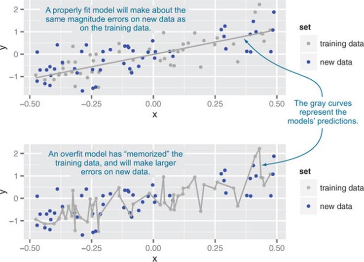
An overly complicated and overfit model is bad for at least two reasons. First, an overfit model may be much more complicated than anything useful. For example, the extra wiggles in the overfit part of figure 5.11 could make optimizing with respect to x needlessly difficult. Also, as we mentioned, overfit models tend to be less accurate in production than during training, which is embarrassing.

5.3.2. Quantifying model soundness

It’s important that you know, quantify, and share how sound your model is. Evaluating a model only on the data used to construct it is favorably biased: models tend to look good on the data they were built from. Also, a single evaluation of model performance gives only a point estimate of performance. You need a good characterization of how much potential variation there is in your model production and measurement procedure, and how well your model is likely to perform on future data. We see these questions as being fundamentally frequentist concerns because they’re questions about how model behavior changes under variations in data. The formal statistical term closest to these business questions is significance, and we’ll abuse notation and call what we’re doing significance testing.^[5] In this section, we’ll discuss some testing procedures, but postpone demonstrating implementation until later in this book.

⁵ A lot of what we’re doing is in fact significance testing. We just re-derive it in small steps to make sure we keep our testing strategy linked in an explainable way to our original business goals.

Frequentist and Bayesian inference

Following Efron,^[6] there are at least two fundamental ways of thinking about inference: frequentist and Bayesian (there are more; for example, Fisherian and information theoretic). In frequentist inference, we assume there is a single unknown fixed quantity (be it a parameter, model, or prediction) that we’re trying to estimate. The frequentist inference for a given dataset is a point estimate that varies as different possible datasets are proposed (yielding a distribution of estimates). In Bayesian inference, we assume that the unknown quantity to be estimated has many plausible values modeled by what’s called a prior distribution. Bayesian inference is then using data (that is considered as unchanging) to build a tighter posterior distribution for the unknown quantity.

⁶ See Bradley Efron, “Controversies In The Foundation Of Statistics,” American Mathematical Monthly, 1978, 85 (4), pp. 231-246.

There’s a stylish snobbery that Bayesian inference is newer and harder to do than frequentist inference, and therefore more sophisticated. It is true that Bayesian methods model the joint nature of parameters and data more explicitly than frequentist methods. And frequentist methods tend to be much more compact and efficient (which isn’t always a plus, as frequentist testing procedures can degenerate into ritual when applied without thought).

In practice, choosing your inference framework isn’t a matter of taste, but a direct consequence of what sort of business question you’re trying to answer. If you’re worried about the sensitivity of your result to variation in data and modeling procedures, you should work in the frequentist framework. If you’re worried about the sensitivity of your result to possible variation in the unknown quantity to be modeled, you should work in the Bayesian framework (see http://mng.bz/eHGj).

5.3.3. Ensuring model quality

The standards of scientific presentation are that you should always share how sensitive your conclusions are to variations in your data and procedures. You should never just show a model and its quality statistics. You should also show the likely distribution of the statistics under variations in your modeling procedure or your data. This is why you wouldn’t say something like “We have an accuracy of 90% on our training data,” but instead you’d run additional experiments so you could say something like “We see an accuracy of 85% on hold-out data.” Or even better: “We saw accuracies of at least 80% on all but 5% of our reruns.” These distributional statements tell you if you need more modeling features and/or more data.

Testing on held-out data

The data used to build a model is not the best data for testing the model’s performance. This is because there’s an upward measurement bias in this data. Because this data was seen during model construction, and model construction is optimizing your performance measure (or at least something related to your performance measure), you tend to get exaggerated measures of performance on your training data. Most standard fitting procedures have some built-in measure for this effect (for example, the “adjusted R-squared” report in linear regression, discussed in section 7.1.5) and the effect tends to diminish as your training data becomes large with respect to the complexity of your model.^[7]

⁷ See, for example, “The Unreasonable Effectiveness of Data,” Alon Halevy, Peter Norvig, and Fernando Pereira, IEEE Intelligent Systems, 2009.

The precaution for this optimistic bias we demonstrate throughout this book is this: split your available data into test and training. Perform all of your clever work on the training data alone, and delay measuring your performance with respect to your test data until as late as possible in your project (as all choices you make after seeing your test or hold-out performance introduce a modeling bias). The desire to keep the test data secret for as long as possible is why we often actually split data into training, calibration, and test sets (as we’ll demonstrate in section 6.1.1).

K-fold cross-validation

Testing on hold-out data, while useful, only gives a single-point estimate of model performance. In practice we want both an unbiased estimate of our model’s future performance on new data (simulated by test data) and an estimate of the distribution of this estimate under typical variations in data and training procedures. A good method to perform these estimates is k-fold cross-validation and the related ideas of empirical resampling and bootstrapping.

The idea behind k-fold cross-validation is to repeat the construction of the model on different subsets of the available training data and then evaluate the model only on data not seen during construction. This is an attempt to simulate the performance of the model on unseen future data. The need to cross-validate is one of the reasons it’s critical that model construction be automatable, such as with a script in a language like R, and not depend on manual steps. Assuming you have enough data to cross-validate (not having to worry too much about the statistical efficiency of techniques) is one of the differences between the attitudes of data science and traditional statistics. Section 6.2.3 works through an example of automating k-fold cross-validation.

Significance testing

Statisticians have a powerful idea related to cross-validation called significance testing. Significance also goes under the name of p-value and you will actually be asked, “What is your p-value?” when presenting.

The idea behind significance testing is that we can believe our model’s performance is good if it’s very unlikely that a naive model (a null hypothesis) could score as well as our model. The standard incantation in that case is “We can reject the null hypothesis.” This means our model’s measured performance is unlikely for the null model. Null models are always of a simple form: assuming two effects are independent when we’re trying to model a relation, or assuming a variable has no effect when we’re trying to measure an effect strength.

For example, suppose you’ve trained a model to predict how much a house will sell for, based on certain variables. You want to know if your model’s predictions are better than simply guessing the average selling price of a house in the neighborhood (call this the null model). Your new model will mispredict a given house’s selling price by a certain average amount, which we’ll call err.model. The null model will also mispredict a given house’s selling price by a different amount, err.null. The null hypothesis is that D = (err.null - err.model) == 0—on average, the new model performs the same as the null model.

When you evaluate your model over a test set of houses, you will (hopefully) see that D = (err.null - err.model) > 0 (your model is more accurate). You want to make sure that this positive outcome is genuine, and not just something you observed by chance. The p-value is the probability that you’d see a D as large as you observed if the two models actually perform the same.

Our advice is this: always think about p-values as estimates of how often you’d find a relation (between the model and the data) when there actually is none. This is why low p-values are good, as they’re estimates of the probabilities of undetected disastrous situations (seehttp://mng.bz/A3G1). You might also think of the p-value as the probability of your whole modeling result being one big “false positive.” So, clearly, you want the p-value (or the significance) to be small, say less than 0.05.

The traditional statistical method of computing significance or p-values is through a Student’s t-test or an f-test (depending on what you’re testing). For classifiers, there’s a particularly good significance test that’s run on the confusion matrix called the fisher.test(). These tests are built into most model fitters. They have a lot of math behind them that lets a statistician avoid fitting more than one model. These tests also rely on a few assumptions (to make the math work) that may or may not be true about your data and your modeling procedure.

One way to directly simulate a bad modeling situation is by using a permutation test. This is when you permute the input (or independent) variables among examples. In this case, there’s no real relation between the modeling features (which we have permuted among examples) and the quantity to be predicted, because in our new dataset the modeling features and the result come from different (unrelated) examples. Thus each rerun of the permuted procedure builds something much like a null model. If our actual model isn’t much better than the population of permuted models, then we should be suspicious of our actual model. Note that in this case, we’re thinking about the uncertainty of our estimates as being a distribution drawn about the null model.

We could modify the code in section 6.2.3 to perform an approximate permutation test by permuting the y-values each time we resplit the training data. Or we could try a package that performs the work and/or brings in convenient formulas for the various probability and significance statements that come out of permutation experiments (for example, http://mng.bz/SvyB).

Confidence intervals

An important and very technical frequentist statistical concept is the confidence interval. To illustrate, a 95% confidence interval is an interval from an estimation procedure such that the procedure is thought to have a 95% (or better) chance of catching the true unknown value to be estimated in an interval. It is not the case that there is a 95% chance that the unknown true value is actually in the interval at hand (thought it’s often misstated as such). The Bayesian alternative to confidence intervals is credible intervals (which can be easier to understand, but do require the introduction of a prior distribution).

Using statistical terminology

The field of statistics has spent the most time formally studying the issues of model correctness and model soundness (probability theory, operations research, theoretical computer science, econometrics, and a few other fields have of course also contributed). Because of their priority, statisticians often insist that the checking of model performance and soundness be solely described in traditional statistical terms. But a data scientist must present to many non-statistical audiences, so the reasoning behind a given test is in fact best explicitly presented and discussed. It’s not always practical to allow the dictates of a single field to completely style a cross-disciplinary conversation.

5.4. Summary

You now have some solid ideas on how to choose among modeling techniques. You also know how to evaluate the quality of data science work, be it your own or that of others. The remaining chapters of part 2 of the book will go into more detail on how to build, test, and deliver effective predictive models. In the next chapter, we’ll actually start building predictive models, using the simplest types of models that essentially memorize and summarize portions of the training data.

Key takeaways

· Always first explore your data, but don’t start modeling before designing some measurable goals.

· Divide you model testing into establishing the model’s effect (performance on various metrics) and soundness (likelihood of being a correct model versus arising from overfitting).

· Keep a portion of your data out of your modeling work for final testing. You may also want to subdivide your training data into training and calibration and to estimate best values for various modeling parameters.

· Keep many different model metrics in mind, and for a given project try to pick the metrics that best model your intended business goal.