From Mathematics to Generic Programming (2011)
11. Permutation Algorithms
An algorithm must be seen to be believed.
Donald Knuth
Complex computer programs are built up from smaller pieces that perform commonly used fundamental tasks. In the previous chapter, we looked at some tasks involving searching for data. In this chapter, we’ll look at tasks that involve shifting data into new positions, and show how to implement them in a generic way. We’ll see how these tasks also end up using two ideas discussed earlier in the book: groups from abstract algebra and the greatest common divisor (GCD) from number theory.
The tasks we will focus on—rotate and reverse—allow us to introduce algorithms that do the same task differently depending on the concept of the iterator to which they apply. In addition to illustrating some generic programming techniques, these algorithms are of great practical importance. The rotate algorithm in particular is probably the most used algorithm inside the implementation of STL components from vector to stable_sort.
11.1 Permutations and Transpositions
Our exploration of the GCD algorithm led us to learn about groups and other algebraic structures. Using this knowledge, we’re going to start investigating the mathematical operations permutation and transposition, which play an important role in some fundamental algorithms.
Definition 11.1. A permutation is a function from a sequence of n objects onto itself.
The formal notation for permutations1 looks like this:
1 This is the same notation mathematicians use for matrices; hopefully the context will make it clear which interpretation is intended.
![]()
The first row represents the indexes (positions) of a sequence of objects; mathematicians start numbering from 1. The second row represents where the items in those positions end up after applying the permutation. In this example, the item that used to be at position 1 will end up in position 2, the item that was in position 2 will end up in position 4, and so on.
In practice, permutations are usually written using a shorthand format that omits the first row:
(2 4 1 3)
In other words, at position i, you write where the ith original element will end up. An example of applying a permutation is
(2 4 1 3) : {a,b,c,d} = {c,a,d,b}
We can use the notion of permutation to define a symmetric group:
Definition 11.2. The set of all permutations on n elements constitutes a group called the symmetric group Sn.
A symmetric group has the following group properties:
binary operation: composition (associative)
inverse operation: inverse permutation
identity element: identity permutation
This is the first example we’ve seen where the elements of a group are themselves functions, and the group operation is an operation on functions. If we have a permutation x that shifts items two positions to the right, and another permutation y that shifts items three positions to the right, then the composition x ![]() y shifts items five positions to the right.
y shifts items five positions to the right.
This is perhaps the most important group to know about, since every finite group is a subgroup of a symmetric group. It is known as Cayley’s Theorem.
Exercise 11.1. Prove Cayley’s Theorem.
Exercise 11.2. What is the order of Sn?
Now let’s look at a special case of permutation, transposition.
Definition 11.3. A transposition (i, j) is a permutation that exchanges the ith and jth elements (i ≠ j), leaving the rest in place.
The notation for transpositions indicates which two positions should get exchanged:
(2 3) : {a,b,c,d} = {a,c,b,d}
In programming, we have a simpler name for transposition: we call it swap. In C++, we might implement it like this:
template <Semiregular T>
void swap(T& x, T& y) {
T tmp(x);
x = y;
y = tmp;
}
The swap operation requires only that the types of its arguments satisfy the concept Semiregular.2 We can see that swap requires the ability to copy-construct, assign, and destruct its data, since those operations are used in the code. It does not need to explicitly test for equality, so we do not need the types to be Regular. When we design an algorithm, we’ll want to know which concepts the types need to satisfy, but we’ll also want to make sure not to impose extra requirements we don’t need.
2 A discussion of C++ move semantics is beyond the scope of this book.
* * *
The transposition lemma demonstrates how fundamental the swap operation is:
Lemma 11.1 (Transposition Lemma): Any permutation is a product of transpositions.
Proof. One transposition can put at least one element into its final destination. Therefore, at most n – 1 transpositions will put all n elements into their final destinations.
![]()
Why do we need only n – 1 transpositions? Because once n – 1 items are in the right place, the nth item must also be in the right place; there’s no place else for it to go.
Exercise 11.3. Prove that if n > 2, Sn is not abelian.
Every permutation defines a directed graph of n elements. After applying the permutation enough times, a given element will eventually be put back in its original position, representing a cycle in the graph. Every permutation can be decomposed into cycles. For example, consider the permutation (2 3 5 6 1 4). The element in position 4 moves to position 6, and the element in position 6 moves to position 4, so after applying the permutation twice, both of those elements will end up where they started. We see a similar pattern for the elements at positions 1, 2, 3, and 5, although this time it takes four operations before they get back to the beginning. We say that the permutation (2 3 5 6 1 4) can be decomposed into two cycles, and we show them graphically like this:
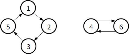
We write this decomposition as (2 3 5 6 1 4) = (1 2 3 5)(4 6).
The cycle notation, used on the right, may be thought of as an extension of the transposition notation. Although the notation is ambiguous (is this a cycle or a permutation?), it is usually clear from the context. Also, permutations always contain all the integers from 1 to n, while cycles might not.
Cycles are disjoint. If you are at a position in a cycle, you can get to all other positions in that cycle. Therefore, if two cycles share one position, they share all positions; that is, they are the same cycle. So the only way to have separate cycles is if they don’t share any positions.
Definition 11.4. A cycle containing one element is called a trivial cycle.
Exercise 11.4. How many nontrivial cycles could a permutation of n elements contain?
Theorem 11.1 (Number of Assignments): The number of assignments needed to perform an arbitrary permutation in place is n – u + v, where n is the number of elements, u is the number of trivial cycles, and v is the number of nontrivial cycles.
Proof. Every nontrivial cycle of length k requires k + 1 assignments, since each element needs to be moved, plus we need to save the first value being overwritten; since every nontrivial cycle requires one extra move, moving all v cycles requires v extra moves. Elements in trivial cycles don’t need to be moved at all, and there are u of those. So we need to move n – u elements, plus v additional moves for the cycles.
![]()
A common permutation that has exactly n/2 cycles is reverse. In some sense this is the “hardest” permutation because it requires the largest number of assignments. We’ll look at reverse in greater detail in the next chapter.
Exercise 11.5. Design an in-place3 reverse algorithm for forward iterators; that is, the algorithm should work for singly linked lists without modifying the links.
3 We’ll discuss the notion of in-place algorithms more in Section 11.6; see Definition 11.6.
11.2 Swapping Ranges
Sometimes we want to swap more than one item at a time. In fact, a common operation in programming is to swap all the values in one range of data with the corresponding values in another (possibly overlapping) range. We do it in a loop, one swap at a time:
Click here to view code image
while (condition) std::swap(*iter0++, *iter1++);
where iter0 and iter1 are iterators pointing to the respective values in each range. Recall from Chapter 10 that we prefer to use semi-open ranges—those where the range includes all elements from the first bound up to but not including the second bound.
When we swap two ranges, often only one of them needs to be specified explicitly. Here, first0 and last0 specify the bounds of the first range, while first1 refers to the start of the second range:
Click here to view code image
template <ForwardIterator I0, ForwardIterator I1>
// ValueType<I0> == ValueType<I1>
I1 swap_ranges(I0 first0, I0 last0, I1 first1) {
while (first0 != last0) swap(*first0++, *first1++);
return first1;
}
There’s no point in specifying the end of the second range, since for the swap to work, it must contain (at least) the same number of elements as the first range. Why do we return first1? Because it might be useful to the caller. For example, if the second range is longer, we might want to know where the unmodified part of the second range begins. It’s information that the caller doesn’t have, and it costs us almost nothing to return.
This is a good time to review the law of useful return, which we introduced in Section 4.6.
The Law of Useful Return, Revisited
When writing code, it’s often the case that you end up computing a value that the calling function doesn’t currently need. Later, however, this value may be important when the code is called in a different situation. In this situation, you should obey the law of useful return:
A procedure should return all the potentially useful information it computed.
The quotient-remainder function that we saw in Chapter 4 is a good example: when we first wrote it, we needed only the remainder, but we had already done all the work to find the quotient. Later, we saw other applications that use both values.
The law does not imply doing unneeded extra computations, nor does it imply that useless information should be returned. For example, in the code given earlier, it’s not useful to return first0, because the algorithm guarantees that at the end it’s equal to last0, which the caller already has. It’s useless to give me information I already have.
The Law of Separating Types
The swap_ranges code illustrates another important programming principle, the law of separating types:
Do not assume that two types are the same when they may be different.
Our function was declared with two iterator types, like this:
Click here to view code image
template <ForwardIterator I0, ForwardIterator I1>
// ValueType<I0> == ValueType<I1>
I1 swap_ranges(I0 first0, I0 last0, I1 first1);
rather than assuming that they’re the same type, like this:
Click here to view code image
template <ForwardIterator I>
I swap_ranges(I first0, I last0, I first1);
The first way gives us more generality and allows us to use the function in situations we wouldn’t otherwise be able to, without incurring any additional computation cost. For example, we could swap a range of elements in a linked list with a range of elements in an array and it would just work.
However, just because two types are distinct does not mean there is no relationship between them. In the case of swap_ranges, for the implementation to be able to call swap on the data, we need to ensure that the value type of I0 is the same as the value type of I1. While the compiler cannot check this condition today, we can indicate it with a comment in the code.
In situations where we’re not sure if the second range is long enough to perform all the needed swaps, we can make both ranges explicit and have our while test check to make sure neither iterator has run off the end of the range:
Click here to view code image
template <ForwardIterator I0, ForwardIterator I1>
std::pair<I0, I1> swap_ranges(I0 first0, I0 last0,
I1 first1, I1 last1) {
while (first0 != last0 && first1 != last1) {
swap(*first0++, *first1++);
}
return {first0, first1};
}
This time we do return both first0 and first1, because one range may be exhausted before the other, so we won’t necessarily have reached last0 and last1.
Swapping counted ranges is almost the same, except that instead of checking to see if we reached the end of the range, we count down from n to 0:
Click here to view code image
template <ForwardIterator I0, ForwardIterator I1, Integer N>
std::pair<I0, I1> swap_ranges_n(I0 first0, I1 first1, N n) {
while (n != N(0)) {
swap(*first0++, *first1++);
--n;
}
return {first0, first1};
}
The Law of Completeness
Observe that we created both swap_ranges and swap_ranges_n. Even though in a particular situation the programmer might need only one of these versions, later on a client might need the other version.
This follows the law of completeness:
When designing an interface, consider providing all the related procedures.
If there are different ways of invoking an algorithm, provide interfaces for those related functions. In our swap example, we’ve already provided two related interfaces for bounded ranges, and we’ll also provide interfaces for counted ranges.
This rule is not saying that you need to have a single interface to handle multiple cases. It’s perfectly fine to have one function for counted ranges and another for bounded ranges. You especially should not have a single interface for disparate operations. For example, just because containers need to provide both “insert element” and “erase element” functionality doesn’t mean your interface should have a single “insert_or_erase” function.
Counted ranges are easier for the compiler, because it knows the number of iterations, called the trip count, in advance. This allows the compiler to make certain optimizations, such as loop unrolling or software pipelining.
Exercise 11.6. Why don’t we provide the following interface?
Click here to view code image
pair<I0, I1> swap_ranges_n(I0 first0, I1 first1, N0 n0, N1 n1)
11.3 Rotation
One of the most important algorithms you’ve probably never heard of is rotate. It’s a fundamental tool used behind the scenes in many common computing applications, such as buffer manipulation in text editors. It implements the mathematical operation rotation.
Definition 11.5. A permutation of n elements by k where k ≥ 0:
(k mod n, k + 1 mod n, ..., k + n – 2 mod n, k + n – 1 mod n)
is called an n by k rotation.
If you imagine all n elements laid out in a circle, we’re shifting each one “clockwise” by k.
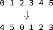
At first glance, it might seem that rotation could be implemented with a modular shift, taking the beginning and end of the range, together with the amount to shift, as arguments. However, doing modular arithmetic on every operation is quite expensive. Also, it turns out that rotation is equivalent to exchanging different length blocks, a task that is extremely useful for many applications. Viewed this way, it is convenient to present rotation with three iterators: f,m, and l, where [f,m) and [m,l) are valid ranges.4 Rotation then interchanges ranges [f,m) and [m,l). If the client wants to rotate k positions in a range [f,l), then it should pass a value of m equal to l – k. As an example, if we want to do a rotation with k = 5 on a sequence specified by the range [0, 7), we choose m = l – k = 7 – 5 = 2:
4 The names f,m, and l are meant to be mnemonics for first, middle, and last.
0 1 2 3 4 5 6
f m l
which produces this result:
2 3 4 5 6 0 1
Essentially, we’re moving each item 5 spaces to the right (and wrapping around when we run off the end).
Exercise 11.7. Prove that if we do rotate(f, m, l), it performs distance(f, l) by distance(m, l) rotation.
An important rotate algorithm was developed by David Gries, a professor at Cornell University, together with IBM scientist Harlan Mills:
Click here to view code image
template <ForwardIterator I>
void gries_mills_rotate(I f, I m, I l) {
// u = distance(f, m) && v = distance(m, l)
if (f == m || m == l) return; // u == 0 || v == 0
pair<I, I> p = swap_ranges(f, m, m, l);
while(p.first != m || p.second != l) {
if (p.first == m) { // u < v
f = m; m = p.second; // v = v - u
} else { // v < u
f = p.first; // u = u - v
}
p = swap_ranges(f, m, m, l);
}
return; // u == v
}
The algorithm first uses the regular swap_ranges function to swap as many elements as we can—as many elements as there are in the shorter range. The if test checks whether we’ve exhausted the first range or the second range. Depending on the result, we reset the start positions of f and m. Then we do another swap, and repeat the process until neither range has remaining elements.
This is easier to follow with an example. Let’s look at how a range is transformed, and how the iterators move, as the algorithm runs:
Start:
0 1 2 3 4 5 6
f m l
Swap [0, 1] and [2, 3]. Have we exhausted both ranges? No, only the first one, so we set f = m and m = p.second, which points to the first element in the sequence that hasn’t yet been moved:
2 3 0 1 4 5 6
f m l
Swap [0, 1] and [4, 5]. Have we exhausted both ranges? No, only the first one, so again we set f = m and m = p.second:
2 3 4 5 0 1 6
f m l
Swap [0] with [6]. Have we exhausted both ranges? No, only the second one this time, so we set f = p.first:
2 3 4 5 6 1 0
f m l
Swap [1] with [0]. Have we exhausted both ranges? Yes, so we’re done.
2 3 4 5 6 0 1
f m
l
Now look at the comments in the gries_mills_rotate code (shown in boldface). We call u the length of the first range [f,m), and v the length of the second range [m,l). We can observe something remarkable: the annotations are performing our familiar subtractive GCD! At the end of the algorithm, u = v = GCD of the lengths of the initial two ranges.
Exercise 11.8. If you examine swap_ranges, you will see that the algorithm does unnecessary iterator comparisons. Rewrite the algorithm so that no unnecessary iterator comparisons are done.
It turns out that many applications benefit if the rotate algorithm returns a new middle: a position where the first element moved. If rotate returns this new middle, then rotate(f, rotate(f, m, l), l) is an identity permutation. First, we need the following “auxiliary rotate” algorithm:
Click here to view code image
template <ForwardIterator I>
void rotate_unguarded(I f, I m, I l) {
// assert(f != m && m != l)
pair<I, I> p = swap_ranges(f, m, m, l);
while (p.first != m || p.second != l) {
f = p.first;
if (m == f) m = p.second;
p = swap_ranges(f, m, m, l);
}
}
The central loop is the same as in the Gries-Mills algorithm, just written differently. (We could have written it this way before but wanted to make the u and v computations clearer.)
We need to find m′—the element whose distance to the last is the same as m’s distance from the first. It’s the value returned by the first call to swap_ranges. To get it back, we can embed a call to rotate_unguarded in our final version of rotate, which works as long as we have forward iterators. As we’ll explain shortly, the forward_iterator_tag type in the argument list will help us invoke this function only in this case:
Click here to view code image
template <ForwardIterator I>
I rotate(I f, I m, I l, std::forward_iterator_tag) {
if (f == m) return l;
if (m == l) return f;
pair<I, I> p = swap_ranges(f, m, m, l);
while (p.first != m || p.second != l) {
if (p.second == l) {
rotate_unguarded(p.first, m, l);
return p.first;
}
f = m;
m = p.second;
p = swap_ranges(f, m, m, l);
}
return m;
}
How much work does this algorithm do? Until the last iteration of the main loop, every swap puts one element in the right place and moves another element out of the way. But in the final call to swap_ranges, the two ranges are the same length, so every swap puts both elements it is swapping into their final positions. In essence, we get an extra move for free on every swap. The total number of swaps is the total number of elements n, minus the number of free swaps we saved in the last step. How many swaps did we save in the last step? The length of the ranges at the end, as we saw earlier, is gcd(n – k,k) = gcd(n,k), where n = distance(f,l) and k = distance(m,l). So the total number of swaps is n – gcd(n,k). Also, since each swap takes three assignments (tmp = a; a = b; b = tmp), the total number of assignments is 3 (n – gcd(n,k)).
11.4 Using Cycles
Can we find a faster rotate algorithm? We can if we exploit the fact that rotations, like any permutations, have cycles. Consider a rotation of k = 2 for n = 6 elements:
The item in position 0 ends up in position 2, 2 ends up in position 4, and 4 ends up back in position 0. These three elements form a cycle. Similarly, item 1 ends up in 3, 3 in 5, and 5 back in 1, forming another cycle. So this rotation has two cycles. Recall from Section 11.1 that we can perform any permutation in n–u+v assignments, where n is the number of elements, u is the number of trivial cycles, and v is the number of nontrivial cycles. Since we normally don’t have any trivial cycles, we need n + v assignments.
Exercise 11.9. Prove that if a rotation of n elements has a trivial cycle, then it has n trivial cycles. (In other words, a rotation either moves all elements or no elements.)
It turns out that the number of cycles is gcd(k,n), so we should be able to do the rotation in n + gcd(k,n) assignments,5 instead of the 3(n – gcd(n,k)) we needed for the Gries-Mills algorithm. Furthermore, in practice GCD is very small; in fact, it is 1 (that is, there is only one cycle) about 60% of the time. So a rotate algorithm that exploits cycles always does fewer assignments.
5 See Elements of Programming, Section 10.4, for the proof.
There is one catch: Gries-Mills only required moving one step forward; it works even for singly linked lists. But if we want to take advantage of cycles, we need to be able to do long jumps. Such an algorithm requires stronger requirements on the iterators—namely, the ability to do random access.
To create our new rotate function, we’ll first write a helper function that moves every element in a cycle to its next position. But instead of saying “which position does the item in position x move to,” we’ll say “in which position do we find the item that’s going to move to position x.” Even though these two operations are symmetric mathematically, it turns out that the latter is more efficient, since it needs only one saved temporary variable per cycle, instead of one for every item that needs to be moved (except the last).
Here’s our helper function:
Click here to view code image
template <ForwardIterator I, Transformation F>
void rotate_cycle_from(I i, F from) {
ValueType<I> tmp = *i;
I start = i;
for (I j = from(i); j != start; j = from(j)) {
*i = *j;
i = j;
}
*i = tmp;
}
Note that we’re using the ValueType type function we defined near the end of Section 10.8.
How does rotate_cycle_from know which position an item comes from? That information will be encapsulated in a function object from that we pass in as an argument. You can think of from(i) as “compute where the element moving into position i comes from.”
The function object we’re going to pass to rotate_cycle_from will be an instance of rotate_transform:
Click here to view code image
template <RandomAccessIterator I>
struct rotate_transform {
DifferenceType<I> plus;
DifferenceType<I> minus;
I m1;
rotate_transform(I f, I m, I l) :
plus(m - f), minus(m - l), m1(f + (l - m)) {}
// m1 separates items moving forward and backward
I operator()(I i) const {
return i + ((i < m1) ? plus : minus);
}
};
The idea is that even though we are conceptually “rotating” elements, in practice some items move forward and some move backward (because the rotation caused them to wrap around the end of our range). When rotate_transform is instantiated for a given set of ranges, it precomputes (1) how much to move forward for items that should move forward, (2) how much to move backward for things that move backward, and (3) what the crossover point is for deciding when to move forward and when to move backward.
Now we can write the cycle-exploiting version of algorithm for rotation, which is a variation of the algorithm discovered by Fletcher and Silver in 1965:
Click here to view code image
template <RandomAccessIterator I>
I rotate(I f, I m, I l, std::random_access_iterator_tag) {
if (f == m) return l;
if (m == l) return f;
DifferenceType<I> cycles = gcd(m - f, l - m);
rotate_transform<I> rotator(f, m, l);
while (cycles-- > 0) rotate_cycle_from(f + cycles, rotator);
return rotator.m1;
}
After handling some trivial boundary cases, the algorithm first computes the number of cycles (the GCD) and constructs a rotate_transform object. Then it calls rotate_cycle_from to shift all the elements along each cycle, and repeats this for every cycle.
Let’s look at an example. Consider the rotation k = 2 for n = 6 elements that we used at the beginning of this section. For simplicity, we’ll assume that our values are integers stored in an array:
0 1 2 3 4 5
We also assume our iterators are integer offsets in an array, starting at 0. (Be careful to distinguish between the values at a position and the position itself.) To perform a k = 2 rotation, we’ll need to pass the three iterators f = 0, m = 4, and l = 6:
0 1 2 3 4 5
f m l
The boundary cases of our new rotate algorithm don’t apply, so the first thing it does is compute the number of cycles, which is equal to gcd(m – f, l – m) = gcd(4, 2) = 2. Then it constructs the rotator object, initializing its state variables as follows:
plus ← m – f = 4 – 0 = 4
minus ← m – l = 4 – 6 = – 2
m1 ← f + (l – m) = 0 + (6 – 4) = 2
The main loop of the function rotates all elements of a cycle, then moves on to the next cycle. Let us see what happens when rotate_cycle_from is called.
Initially, we pass f + d = 0 + 2 = 2 as the first argument. So inside the function, i = 2. We save the value at position 2, which is also 2, to our tmp variable and set start to our starting position of 2.
Now we go through a loop as long as a new variable, j, is not equal to start. Each time through the loop, we are going to set j by using the rotator function object that we passed in through the variable from. Basically, all that object does is add the stored values plus or minus to its argument, depending on whether the argument is less than the stored value m1. For example, if we call from(0), it will return 0 + 4, or 4, since 0 is less than 2. If we call from(4), it will return 4 + (–2), or 2, since 4 is not less than 2.
Here’s how the values in our array change as we go through the loop in rotate_cycle_from:
i ← 2, j ← from(2) = 0
0 1 2 3 4 5
j i
*i ← *j
0 1 0 3 4 5
j i
i ← j = 0, j ← from(0) = 4
0 1 0 3 4 5
i j
*i ← *j
4 1 0 3 4 5
i j
i ← j = 4, j ← from (4) = 2 which is start, so loop ends
4 1 0 3 4 5
j i
*i ← tmp
4 1 0 3 2 5
j i
This completes the first call to rotate_cycle_from in the while loop of our rotate function.
Exercise 11.10. Continue to trace the preceding example until the rotate function finishes.
Notice that the signatures of this rotate function and the previous one differ by the type of the last argument. In the next section, we’ll write the wrapper that lets the fastest implementation for a given situation be automatically invoked.
When Is an Algorithm Faster in Practice?
We have seen an example where one algorithm does fewer assignments than another algorithm. Does that mean it will run faster? Not necessarily. In practice, the ability to fit relevant data in cache can make a dramatic difference in this speed. An algorithm that involves large jumps in memory—that is, one that has poor locality of reference—may end up being slower than one that requires more assignments but has better locality of reference.
11.5 Reverse
Another fundamental algorithm is reverse, which (obviously) reverses the order of the elements of a sequence. More formally, reverse permutes a k-element list such that item 0 and item k − 1 are swapped, item 1 and item k − 2 are swapped, and so on.
If we have reverse, we can implement rotate in just three lines of code:
Click here to view code image
template <BidirectionalIterator I>
void three_reverse_rotate(I f, I m, I l) {
reverse(f, m);
reverse(m, l);
reverse(f, l);
}
For example, suppose we want to perform our k = 2 rotation on the sequence 0 1 2 3 4 5. The algorithm would perform the following operations:
Click here to view code image
f m l
start 0 1 2 3 4 5
reverse(f, m) 3 2 1 0 4 5
reverse(m, l) 3 2 1 0 5 4
reverse(f, l) 4 5 0 1 2 3
Exercise 11.11. How many assignments does 3-reverse rotate perform?
This elegant algorithm, whose inventor is unknown, works for bidirectional iterators. However, it has one problem: it doesn’t return the new middle position. To solve this, we’re going to break the final reverse call into two parts. We’ll need a new function that reverses elements until one of the two iterators reaches the end:
Click here to view code image
template <BidirectionalIterator I>
pair<I, I> reverse_until(I f, I m, I l) {
while (f != m && m != l) swap(*f++, *--l);
return {f, l};
}
At the end of this function, the iterator that didn’t hit the end will be pointing to the new middle.
Now we can write a general rotate function for bidirectional iterators. When it gets to what would have been the third reverse call, it does reverse_until instead, saves the new middle position, and then finishes reversing the rest of the range:
Click here to view code image
template <BidirectionalIterator I>
I rotate(I f, I m, I l, bidirectional_iterator_tag) {
reverse(f, m);
reverse(m, l);
pair<I, I> p = reverse_until(f, m, l);
reverse(p.first, p.second);
if (m == p.first) return p.second;
return p.first;
}
We have seen three different implementations of rotate, each optimized for different types of iterators. However, we’d like to hide this complexity from the programmer who’s going to be using these functions. So, just as we did with the distance functions in Section 10.5, we’re going to write a simpler version that works for any type of iterator, and use category dispatch to let the compiler decide which implementation will get executed:
Click here to view code image
template <ForwardIterator I>
I rotate(I f, I m, I l) {
return rotate(f, m, l, IteratorCategory<I>());
}
The programmer just needs to call a single rotate function; the compiler will extract the type of the iterator being used and invoke the appropriate implementation.
* * *
We’ve been using a reverse function, but how might we implement it? For bidirectional iterators, the code is fairly straightforward; we have a pointer to the beginning that moves forward, and a pointer to the end that moves backward, and we keep swapping the elements they point to until they run into each other:
Click here to view code image
template <BidirectionalIterator I>
void reverse(I f, I l, std::bidirectional_iterator_tag) {
while (f != l && f != --l) std::swap(*f++, *l);
}
Exercise 11.12. Explain why we need two tests per iteration in the preceding while loop.
It might appear that according to the law of useful return we should return pair<I, I>(f, l). However, there is no evidence that this information is actually useful; therefore the law does not apply.
Of course, if we already knew in advance how many times we had to execute the loop (the trip count), we wouldn’t need two comparisons. If we pass the trip count n to our function, we can implement it with only n/2 tests:
Click here to view code image
template <BidirectionalIterator I, Integer N>
void reverse_n(I f, I l, N n) {
n >>= 1;
while (n-- > N(0)) {
swap(*f++, *--l);
}
}
In particular, if we have a random access iterator, we can compute the trip count in constant time, and implement reverse using reverse_n, like this:
Click here to view code image
template <RandomAccessIterator I>
void reverse(I f, I l, std::random_access_iterator_tag) {
reverse_n(f, l, l - f);
}
What if we have only forward iterators and we still want to reverse? We’ll use a recursive auxiliary function that keeps partitioning the range in half (the h in the code). The argument n keeps track of the length of the sequence being reversed:
Click here to view code image
template <ForwardIterator I, Integer N>
I reverse_recursive(I f, N n) {
if (n == 0) return f;
if (n == 1) return ++f;
N h = n >> 1;
I m = reverse_recursive(f, h);
if (odd(n)) ++m;
I l = reverse_recursive(m, h);
swap_ranges_n(f, m, h);
return l;
}
Exercise 11.13. Using the sequence {0, 1, 2, 3, 4, 5, 6, 7, 8} as an example, trace the operation of the reverse_recursive algorithm.
The function returns the end of the range, so the first recursive call returns the midpoint. Then we advance the midpoint by 1 or 0 depending on whether the length is even or odd.
Now we can write our reverse function for forward iterators:
Click here to view code image
template <ForwardIterator I>
void reverse(I f, I l, std::forward_iterator_tag) {
reverse_recursive(f, distance(f, l));
}
Finally, we can write the generic version of reverse that works for any iterator type, just as we did for rotate earlier:
Click here to view code image
template <ForwardIterator I>
void reverse(I f, I l) {
reverse(f, l, IteratorCategory<I>());
}
The Law of Interface Refinement
What is the correct interface for rotate? Originally, std::rotate returned void. After several years of usage, it became clear that returning the new middle (the position where the first element moved) made implementation of several other STL algorithms, such as in_place_merge and stable_partition, simpler.
Unfortunately, it was not immediately obvious how to return this value without doing any extra work. Only after this implementation problem was solved was it possible to redesign the interface to return the required value. It then took more than 10 years to change the C++ language standard.
This is a good illustration of the law of interface refinement:
Designing interfaces, like designing programs, is a multi-pass activity.
We can’t really design an ideal interface until we have seen how the algorithm will be used, and not all the uses are immediately apparent. Furthermore, we can’t design an ideal interface until we know which implementations are feasible.
11.6 Space Complexity
When talking about concrete algorithms, programmers need to think about where they fall in terms of time and space complexity. There are many levels of time complexity (e.g., constant, logarithmic, quadratic). However, the traditional view of space complexity put algorithms into just two categories: those that perform their computations in place and those that do not.
Definition 11.6. An algorithm is in-place (also called polylog space) if for an input of length n it uses O((log n)k) additional space, where k is a constant.
Initially, in-place algorithms were often defined as using constant space, but this was too narrow a restriction. The idea of being “in place” was supposed to capture algorithms that didn’t need to make a copy of their data. But many of these non-data-copying algorithms, like quicksort, use a divide-and-conquer technique that requires logarithmic extra space. So the definition was formalized in a way that included these algorithms.
Algorithms that are not in-place use more space—usually, enough to create a copy of their data.
* * *
Let’s use our reverse problem to see how a non-in-place algorithm can be faster than an in-place algorithm. First, we need this helper function, which copies elements in reverse order, starting at the end of a range:
Click here to view code image
template <BidirectionalIterator I, OutputIterator O>
O reverse_copy(I f, I l, O result) {
while (f != l) *result++ = *--l;
return result;
}
Now we can write a non-in-place reverse algorithm. It copies all the data to a buffer, then copies it back in reverse order:
Click here to view code image
template <ForwardIterator I, Integer N, BidirectionalIterator B>
I reverse_n_with_buffer(I f, N n, B buffer) {
B buffer_end = copy_n(f, n, buffer);
return reverse_copy(buffer, buffer_end, f);
}
This function takes only 2n assignments, instead of the 3n we needed for the swap-based implementations.
11.7 Memory-Adaptive Algorithms
In practice, the dichotomy of in-place and non-in-place algorithms is not very useful. While the assumption of unlimited memory is not realistic, neither is the assumption of only polylog extra memory. Usually 25%, 10%, 5%, or at least 1% of extra memory is available and can be exploited to get significant performance gains. Algorithms need to adapt to however much memory is available; they need to be memory adaptive.
Let’s create a memory-adaptive algorithm for reverse. It takes a buffer that we can use as temporary space, and an argument bufsize indicating how big the buffer is. The algorithm is recursive—in fact, it’s almost identical to the reverse_recursive function in the previous section. But the recursion happens only on large chunks, so the overhead is acceptable. The idea is that for a given invocation of the function, if the length of the sequence being reversed fits in the buffer, we do the fast reverse with buffer. If not, we recurse, splitting the sequence in half:
Click here to view code image
template <ForwardIterator I, Integer N, BidirectionalIterator B>
I reverse_n_adaptive(I f, N n, B buffer, N bufsize) {
if (n == N(0)) return f;
if (n == N(1)) return ++f;
if (n <= bufsize) return reverse_n_with_buffer(f, n, buffer);
N h = n >> 1;
I m = reverse_n_adaptive(f, h, buffer, bufsize);
advance(m, n & 1);
I l = reverse_n_adaptive(m, h, buffer, bufsize);
swap_ranges_n(f, m, h);
return l;
}
The caller of this function should ask the system how much memory is available, and pass that value as bufsize. Unfortunately, such a call is not provided in most operating systems.
A Sad Story about get_temporary_buffer
When the C++ STL library was designed by the first author of this book, he realized that it would be helpful to have a function get_temporary_buffer that takes a size n and returns the largest available temporary buffer up to size n that fits into physical memory. As a placeholder (since the correct version needs to have knowledge that only the operating system has), he wrote a simplistic and impractical implementation, which repeatedly calls malloc asking for initially huge and gradually smaller chunks of memory until it returns a valid pointer. He put in a prominent comment in the code saying something like, “This is a bogus implementation, replace it!” To his surprise, he discovered years later that all the major vendors that provide STL implementations are still using this terrible implementation—but they removed his comment.
11.8 Thoughts on the Chapter
One of the things we’ve seen in both this chapter and the previous one is how simple computational tasks offer rich opportunities to explore different algorithms and learn from them. The programming principles that arise from these examples—the laws of useful return, separating types, completeness, and interface refinement—carry over into nearly every programming situation.
This chapter has also presented some good examples of how theory and practice come together in programming. Our knowledge of the theory of permutations—itself based on group theory—allowed us to come up with a more efficient algorithm for rotation, one that exploited the properties that our theory guaranteed. At the same time, the example of memory-adaptive algorithms demonstrated how practical considerations such as the amount of available memory can have a profound impact on the choice of algorithm and its performance. Theory and practice are two sides of the same coin; good programmers rely on knowledge of both.
All materials on the site are licensed Creative Commons Attribution-Sharealike 3.0 Unported CC BY-SA 3.0 & GNU Free Documentation License (GFDL)
If you are the copyright holder of any material contained on our site and intend to remove it, please contact our site administrator for approval.
© 2016-2026 All site design rights belong to S.Y.A.