From Mathematics to Generic Programming (2011)
12. Extensions of GCD
I swear by the even and the odd.
Quran, Surah Al-Fajr
Programmers often assume that since a data structure or algorithm is in a textbook or has been used for years, it represents the best solution to a problem. Surprisingly, this is often not the case—even if the algorithm has been used for thousands of years and has been worked on by everyone from Euclid to Gauss. In this chapter we’ll look at an example of a novel solution to an old problem—computing the GCD. Then we’ll see how proving a theorem from number theory resulted in an important variation of the algorithm still used today.
12.1 Hardware Constraints and a More Efficient Algorithm
In 1961, an Israeli Ph.D. student, Josef “Yossi” Stein, was working on something called Racah Algebra for his dissertation. He needed to do rational arithmetic, which required reducing fractions, which uses the GCD. But because he had only limited time on a slow computer, he was motivated to find a better way. As he explains:
Using “Racah Algebra” meant doing calculations with numbers of the form a/b. ![]() , where, a, b, c were integers. I wrote a program for the only available computer in Israel at that time—the WEIZAC at the Weizmann institute. Addition time was 57 microseconds, division took about 900 microseconds. Shift took less than addition.... We had neither compiler nor assembler, and no floating-point numbers, but used hexadecimal code for the programming, and had only 2 hours of computer-time per week for Racah and his students, and you see that I had the right conditions for finding that algorithm. Fast GCD meant survival.1
, where, a, b, c were integers. I wrote a program for the only available computer in Israel at that time—the WEIZAC at the Weizmann institute. Addition time was 57 microseconds, division took about 900 microseconds. Shift took less than addition.... We had neither compiler nor assembler, and no floating-point numbers, but used hexadecimal code for the programming, and had only 2 hours of computer-time per week for Racah and his students, and you see that I had the right conditions for finding that algorithm. Fast GCD meant survival.1
1 J. Stein, personal communication, 2003.
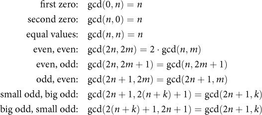
What Stein observed was that there were certain situations where the GCD could be easily computed, or easily expressed in terms of another GCD expression. He looked at special cases like taking the GCD of an even number and an odd number, or a number and itself. Eventually, he came up with the following exhaustive list of cases:
Using these observations, Stein wrote the following algorithm:
Click here to view code image
template <BinaryInteger N>
N stein_gcd(N m, N n) {
if (m < N(0)) m = -m;
if (n < N(0)) n = -n;
if (m == N(0)) return n;
if (n == N(0)) return m;
// m > 0 && n > 0
int d_m = 0;
while (even(m)) { m >>= 1; ++d_m;}
int d_n = 0;
while (even(n)) { n >>= 1; ++d_n;}
// odd(m) && odd(n)
while (m != n) {
if (n > m) swap(n, m);
m -= n;
do m >>= 1; while (even(m));
}
// m == n
return m << min(d_m, d_n);
}
Let’s look at what the code is doing. The function takes two BinaryIntegers—that is, an integer representation that supports fast shift and even/odd testing, like typical computer integers. First, it eliminates the easy cases where one of the arguments is zero, and inverts the sign if an argument is negative, so that we are dealing with two positive integers.
Next, it takes advantage of the identities with even arguments, removing factors of 2 (by shifting) while keeping track of how many there were. We can use a simple int for the counts, since what we’re counting is at most the total number of bits in the original arguments. After this part, we are operating on two odd numbers.
Now comes the main loop. We repeatedly subtract the smaller from the larger each time (since we know the difference of two odd numbers is even), and again use shifts to remove additional powers of 2 from the result.2 When we’re done, our two numbers will be equal. Since we’re halving at least once each time through the loop, we know we’ll iterate no more than log n times; the algorithm is bounded by the number of 1-bits we encounter.
2 We use do-while rather than while because we don’t need to run the the test the first time; we know we’re starting with an even number so we know we have to do at least one shift.
Finally, we return our result, using a shift to multiply our number by 2 for each of the minimum number of 2s we factored out at the beginning. We don’t need to worry about 2s in the main loop, because by that point we’ve reduced the problem to the GCD of two odd numbers; this GCD does not have 2 as a factor.
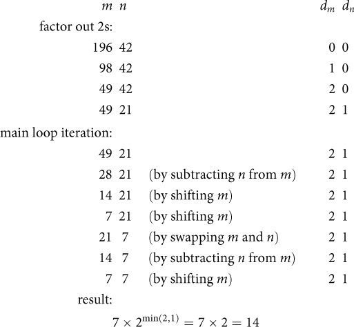
Here’s an example of the algorithm in operation. Suppose we want to compute GCD(196, 42). The computation looks like this:
As we saw, Stein took some observations about special cases and turned them into a faster algorithm. The special cases had to do with even and odd numbers, and places where we could factor out 2, which is easy on a computer; that’s why Stein’s algorithm is faster in practice. (Even today, when the remainder function can be computed in hardware, it is still much slower than simple shifts.) But is this just a clever hack, or is there more here than meets the eye? Does it make sense only because computers use binary arithmetic? Does Stein’s algorithm work just for integers, or can we generalize it just as we did with Euclid’s algorithm?
12.2 Generalizing Stein’s Algorithm
To answer these questions, let’s review some of the historical milestones for Euclid’s GCD:
• Positive integers: Greeks (5th century BC)
• Polynomials: Stevin (ca. 1600)
• Gaussian integers: Gauss (ca. 1830)
• Algebraic integers: Dirichlet, Dedekind (ca. 1860)
• Generic version: Noether, van der Waerden (ca. 1930)
It took more than 2000 years to extend Euclid’s algorithm from integers to polynomials. Fortunately, it took much less time for Stein’s algorithm. In fact, just 2 years after its publication, Knuth already knew of a version for single-variable polynomials over a field ![]() .
.
The surprising insight was that we can have x play the role for polynomials that 2 plays for integers. That is, we can factor out powers of x, and so on. Carrying the analogy further, we see that x2 + x (or anything else divisible by x) is “even,” x2 + x + 1 (or anything else with a zero-order coefficient) is “odd,” and x2 + x “shifts” to x + 1. Just as division by 2 is easier than general division for binary integers, so division by x is easier than general division for polynomials—in both cases, all we need is a shift. (Remember that a polynomial is really a sequence of coefficients, so division by x is literally a shift of the sequence.)
Stein’s “special cases” for polynomials look like this:
![]()
![]()
![]()
![]()
![]()
![]()
![]()
Notice how each of the last two rules cancels one of the zero-order coefficients, so we convert the “odd, odd” case to an “even, odd” case.
To get the equivalence expressed by Equation 12.6, we rely on two facts. First, if you have two polynomials u and v, then gcd(u,v) = gcd(u,av), where a is a nonzero coefficient. So we can multiply the second argument by the coefficient ![]() , and we’ll have the same GCD:
, and we’ll have the same GCD:
![]()
Second, gcd(u,v) = gcd(u,v - u), which we noted when we introduced GCD early in the book (Equation 3.9). So we can subtract our new second argument from the first, and we’ll still have the same GCD:
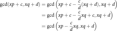
Finally, we can use the fact that if one of the GCD arguments is divisible by x and the other is not, we can drop x because the GCD will not contain it as a factor. So we “shift” out the x, which gives
![]()
which is what we wanted.
We also see that in each transformation, the norm—in this case, the degree of the polynomial—gets reduced. Here’s how the algorithm would compute gcd(x3 – 3x – 2, x2 – 4):
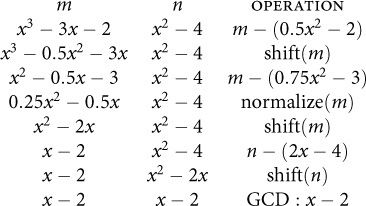
First we see that the ratio of their free coefficients (the c and d in Equations 12.6 and 12.7) is 1/2, so we will multiply n by 1/2 and subtract it from m (shown in the first line of the preceding table), resulting in the new m shown on the second line. Then we “shift” m by factoring out x, resulting in the third line, and so on.
In 2000, Andre Weilert further generalized Stein’s algorithm to Gaussian integers. This time, 1 + i plays the role of 2; the “shift” operation is division by 1 + i. In 2003, Damgård and Frandsen extended the algorithm to Eisenstein integers.
In 2004, Agarwal and Frandsen demonstrated that there is a ring that is not a Euclidean domain, but where the Stein algorithm still works. In other words, there are cases where Stein’s algorithm works but Euclid’s does not. If the domain of the Stein algorithm is not the Euclidean domain, then what is it? As of this writing, this is an unsolved problem.
What we do know is that Stein’s algorithm depends on the notion of even and odd; we generalize even to be divisible by a smallest prime, where p is a smallest prime if any remainder when dividing by it is either zero or an invertible element. (We say “a smallest prime” rather than “the smallest prime” because there could be multiple smallest primes in a ring. For example, for Gaussian integers, 1 + i, 1 – i, – 1 + i, and – 1 – i are all smallest primes.)
Why do we factor out 2 when we’re computing the GCD of integers? Because when we repeatedly divide by 2, we eventually get 1 as a remainder; that is, we have an odd number. Once we have two odd numbers (two numbers whose remainders modulo 2 are both units), we can use subtraction to keep our GCD algorithm going. This ability to cancel remainders works because 2 is the smallest integer prime. Similarly, x is the smallest prime for polynomials, and i + 1 for Gaussian integers.3 Division by the smallest prime always gives a remainder of zero or a unit, because a unit is the number with the smallest nonzero norm. So 2 works for integers because it’s the smallest prime, not because computers use binary arithmetic. The algorithm is possible because of fundamental properties of integers, not because of the hardware implementation, although the algorithm is efficient because computers use binary arithmetic, making shifts fast.
3 Note that 2 is not prime in the ring of Gaussian integers, since it can be factored into (1+i) (1-i).
Exercise 12.1. Compare the performance of the Stein and Euclid algorithms on random integers from the ranges [0, 216), [0, 232), and [0, 264).
12.3 Bézout’s Identity
To understand the relationship of GCD and ring structures, we need to introduce Bézout’s identity, which also leads to an important practical algorithm for computing the multiplicative inverse. The identity says that for any two values a and b in the Euclidean domain, there exist coefficients such that the linear combination gives the GCD of the original values.
Theorem 12.1 (Bézout’s Identity):
![]()
For example, if a = 196 and b = 42, then this says there are values x and y such that 196x + 42y = gcd(196, 42). Since gcd(196, 42) = 14, in this case x = – 1 and y = 5. We’ll see later in the chapter how to compute x and y in general.
Like many results in mathematics, this one is named after someone other than its discoverer. Although 18th-century French mathematician Étienne Bézout did prove the result for polynomials, it was actually shown first for integers a hundred years earlier, by Claude Bachet.
Claude Gaspar Bachet de Méziriac (1581–1638)
Claude Gaspar Bachet de Méziriac, generally known as Bachet, was a French mathematician during the Renaissance. Although he was a scholar in many fields, he is best known for two things. First, he translated Diophantus’ Arithmetic from Greek to Latin, the common language of science and philosophy in Europe at the time. It is his 1621 translation that most mathematicians relied on, and it was in a copy of his translation that Fermat famously wrote the marginal note describing his last theorem. Second, Bachet wrote the first book on recreational mathematics, Problèmes Plaisants, originally published in 1612. Through this book, mathematics became a popular topic among educated people in France, something they would discuss and spend time on as a hobby. Problèmes Plaisants introduced magic squares, as well as proving what is now known as Bézout’s identity.
Bachet was chosen as one of the original members of Académie Française (French Academy), the organization created by Cardinal Richelieu to be the ultimate authority on the French language, and tasked with the creation and maintenance of the official French dictionary.
Recall that a ring is an algebraic structure that behaves similar to integers; it has both plus-like and times-like operations, but only an additive inverse. (You can review the definition of a ring in Definition 8.3 in Section 8.4.)
To prove Bézout’s identity, we need to show that the coefficients x and y always exist. To do this, we need to introduce a new algebraic structure, the ideal.
Definition 12.1. An ideal I is a nonempty subset of a ring R such that
1. ∀x, y ![]() I : x + y
I : x + y ![]() I
I
2. ∀x ![]() I, ∀a
I, ∀a ![]() R : ax
R : ax ![]() I
I
The first property says that the ideal is closed under addition; in other words, if you add any two elements of the ideal, the result is in the ideal. The second property is a bit more subtle; it says that the ideal is closed under multiplication with any element of the ring, not necessarily an element of the ideal.
An example of an ideal is the set of even numbers, which are a nonempty subset of the ring of integers. If you add two even numbers, you get an even number. If you multiply an even number by any number (not necessarily even), you still get an even number. Other examples of ideals are univariate polynomials with root 5, and polynomials with x and y and free coefficient 0 (e.g., x2 + 3y2 + xy + x); we’ll see shortly why this last case is important. Note that just because something is a subring doesn’t mean it’s an ideal. Integers are a subring of Gaussian integers, but they aren’t an ideal of Gaussian integers, because multiplying an integer by the imaginary number i does not produce an integer.
Exercise 12.2.
1. Prove that an ideal I is closed under subtraction.
2. Prove that I contains 0.
Lemma 12.1 (Linear Combination Ideal): In a ring, for any two elements a and b, the set of all elements {xa + yb} forms an ideal.
Proof. First, this set is closed under addition:
(x1a + y1b) + (x2a + y2b) = (x1 + x2)a + (y1 + y2) b
Next, it is closed under multiplication by an arbitrary element:
z(xa + yb) = (zx) a + (zy) b
Therefore, it is an ideal.
![]()
Exercise 12.3. Prove that all the elements of a linear combination ideal are divisible by any of the common divisors of a and b.
Lemma 12.2 (Ideals in Euclidean Domains): Any ideal in a Euclidean domain is closed under the remainder operation and under Euclidean GCD.
Proof.
1. Closed under remainder: By definition,
remainder (a, b) = a – quotient (a, b) · b
If b is in the ideal, then by the second axiom of ideals, anything multiplied by b is in the ideal, so quotient (a, b) · b is in the ideal. By Exercise 12.2, the difference of two elements of an ideal is in the ideal.
2. Closed under GCD: Since the GCD algorithm consists of repeatedly applying remainder, this immediately follows from 1.
![]()
Definition 12.2. An ideal I of the ring R is called a principal ideal if there is an element a ![]() R called the principal element of I such that
R called the principal element of I such that
x ![]() I
I ![]() ∃y
∃y ![]() R : x = ay
R : x = ay
In other words, a principal ideal is an ideal that can be generated from one element. An example of a principal ideal is the set of even numbers (2 is the principal element). Polynomials with root 5 are another principal ideal. In contrast, polynomials with x and y and free coefficient 0 are ideals, but not principal ideals. Remember the polynomial x2 + 3y2 + xy + x, which we gave as an example of an ideal? There’s no way to generate it starting with just x (it would never contain y), and vice versa.
Exercise 12.4. Prove that any element in a principal ideal is divisible by the principal element.
Recall that an integral domain is a ring with no zero divisors (Definition 8.7).
Definition 12.3. An integral domain is called a principal ideal domain (PID) if every ideal in it is a principal ideal.
For example, the ring of integers is a PID, while the ring of multivariate polynomials over integers is not.
Theorem 12.2: ED ![]() PID. Every Euclidean domain is a principal ideal domain.
PID. Every Euclidean domain is a principal ideal domain.
Proof. Any ideal I in a Euclidean domain contains an element m with a minimal positive norm (a “smallest nonzero element”). Consider an arbitrary element a ![]() I; either it is a multiple of m or it has a remainder r:
I; either it is a multiple of m or it has a remainder r:
![]()
But we chose m as the smallest element, so we cannot have a smaller remainder—that would be a contraction. Therefore our element a can’t have a remainder; a = qm. So we can obtain every element from one element, which is the definition of a PID.
![]()
Now we can prove Bézout’s identity. Since it says that there is at least one value of x and one value of y that satisfy the equation xa + yb = gcd(a,b), we can restate it as saying that the set of all possible linear combinations xa + yb contains the desired value.
Bézout’s Identity, Restated: A linear combination ideal I = {xa + yb} of a Euclidean domain contains gcd(a,b).
Proof. Consider the linear combination ideal I = {xa + yb}. a is in I because a = 1a + 0b. Similarly, b is in I because b = 0a + 1b. By Lemma 12.2, any ideal in a Euclidean domain is closed under the GCD; thus gcd(a,b) is in I.
![]()
We can also use Bézout’s identity to prove the Invertibility Lemma, which we encountered in Chapter 5:
Lemma 5.4 (Invertibility Lemma):
![]()
Proof. By Bézout’s identity,
∃x, y ![]()
![]() : xa + yn = gcd(a, n)
: xa + yn = gcd(a, n)
So if gcd(a, n) = 1, then xa + yn = 1. Therefore, xa = –yn + 1, and
xa = 1 mod n
![]()
Exercise 12.5. Using Bézout’s identity, prove that if p is prime, then any 0 < a < p has a multiplicative inverse modulo p.
12.4 Extended GCD
The proof of Bézout’s identity that we saw in the last section is interesting. It shows why the result must be true, but it doesn’t actually tell us how to find the coefficients. This is an example of a nonconstructive proof. For a long time, there was a debate in mathematics about whether nonconstructive proofs were as valid as constructive proofs. Those who opposed the use of nonconstructive proofs were known as constructivists or intuitionists. At the turn of the 20th century, the tide turned against the constructivists, with David Hilbert and the Göttingen school leading the charge. The lone major defender of constructivism, Henri Poincaré, lost the battle, and today nonconstructive proofs are routinely used.
Henri Poincaré (1854–1912)
Jules Henri Poincaré was a French mathematician and physicist. He came from a deeply patriotic family, and his cousin Raymond was a prime minister of France. He published more than 500 papers on a variety of subjects, including several on special relativity developed independently of, and in some cases prior to, Einstein’s work on the subject. Although he worked on many practical problems, such as establishing time zones, he mostly valued science as a tool for understanding the universe.
As he wrote:
The scientist must not dally in realizing practical aims. He no doubt will obtain them, but must obtain them in addition. He never must forget that the special object he is studying is only a part of this big whole, which must be the sole motive of his activity. Science has had marvelous applications, but a science that would only have applications in mind would not be science anymore, it would be only cookery.
Poincaré also wrote several important books about the philosophy of science, and was elected a member of the Académie Française.
Poincaré contributed to almost every branch of mathematics, originating several subfields, such as algebraic topology. People at the time debated about whether Poincaré or Hilbert was the greatest mathematician in the world. However, Poincaré’s criticism of set theory and the formalist agenda of Hilbert put him on the wrong side of the rivalry between France and a recently unified Germany. The rejection of Poincaré’s intuitionist approach by the formalists was a great loss for 20th-century mathematics. Both points of view complement each other.
Whatever the view of formalist mathematicians, from a programming perspective, it is clearly more satisfactory to actually have an algorithm than simply to know that one exists. So in this section, we will derive a constructive proof of Bézout’s identity—in other words, an algorithm for finding x and y such that xa + yb = gcd(a,b).
To understand the process, it’s helpful to review what happens in several iterations of Euclid’s algorithm to compute the GCD of a and b.
Click here to view code image
template <EuclideanDomain E>
E gcd(E a, E b) {
while (b != E(0)) {
a = remainder(a, b);
std::swap(a, b);
}
return a;
}
Each time through the main loop, we replace a by the remainder of a and b, then swap a and b; our final remainder will be the GCD. So we are computing this sequence of remainders:
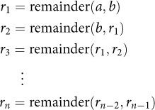
Note how the second argument to the remainder function on iteration k shifts over to become the first argument on iteration k + 1.
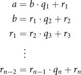
Since the remainder of a and b is what’s left over from a after dividing a by b, we can write the sequence like this:
![]()
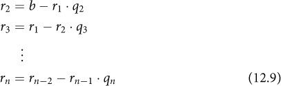
where the q terms are the corresponding quotients. We can solve each equation for the first term on the right—the first argument of the remainder function:
In Section 4.7, we showed how the last nonzero remainder rn in the sequence is equal to the GCD of the original arguments. For Bézout’s identity, we’d like to show that rn = gcd(a,b) = xa + yb. If each of the equations in the preceding series could be written as linear combinations of a and b, the next one could as well. The first three are easy:
![]()
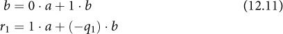
The last equation comes from our original definition of r1 in the first remainder sequence (Equation 12.8). The next one requires substituting the expansion of r1 and rearranging terms:
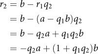
Next, we have an iterative recurrence. Assume that we already figured out how to represent two successive remainders as linear combinations:
ri = xia + yib
ri+1 = xi+1a + yi+1b
Then we can use our previous observation about how to define an arbitrary remainder in the sequence using the two previous ones (Equation 12.9), substituting those previous values and again distributing and rearranging to group all the coefficients with a and all the coefficients with b:
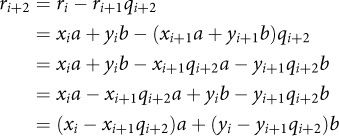
We have seen how we can express every entry in the sequence as a linear combination of a and b, and our procedure gives us the coefficients x and y at every step. Furthermore, we observe that the coefficients on a are defined in terms of the previous coefficients on a (i.e., the only variables are xs), and the coefficients on b are defined in terms of the previous coefficients on b (i.e., the only variables are ys). In particular, the coefficients on iteration i + 2 are
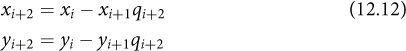
When we reach the end, we have coefficients x and y such that xa + yb = gcd(a,b), which was what we wanted all along.
We’ve seen that that the ys do not depend on the xs and the xs do not depend on the ys. Since we know xa + yb = gcd(a,b), then as long as b ≠ 0, we can rearrange these terms to define y as
![]()
This means we don’t need to go through the trouble of computing all the intermediate values of y.
Exercise 12.6. What are x and y if b = 0?
* * *
Now that we know how to compute the coefficient x from Bézout’s identity, we can enhance our GCD algorithm to return this value as well. The new algorithm is called extended GCD (also known as the extended Euclid algorithm). It will still compute the usual series of remainders for GCD, but it will also compute the series of x coefficients from our earlier equations.
As we have seen, we don’t need to keep every value in the recurrence; we just need the two previous ones, which we’ll call x0 and x1. Of course, we need to know the first two values to get the series started, but fortunately we have them—they are the coefficients of a in the first two linear combinations (Equations 12.10 and 12.11), namely 1 and 0. Then we can use the xi+2 formula we have just derived (Equation 12.12) to compute the new value each time. Each new x computation requires a quotient, so we’ll need a function for that. Meanwhile we’re still computing the GCD, so we still need the remainder. Since we need both quotient and remainder, we’ll use the generic version of the quotient_remainder function we introduced in Section 4.6, which returns a pair whose first element is the quotient and whose second element is the remainder. Here is our extended GCD code:
Click here to view code image
template <EuclideanDomain E>
std::pair<E, E> extended_gcd(E a, E b) {
E x0(1);
E x1(0);
while (b != E(0)) {
// compute new r and x
std::pair<E, E> qr = quotient_remainder(a, b);
E x2 = x0 - qr.first * x1;
// shift r and x
x0 = x1;
x1 = x2;
a = b;
b = qr.second;
}
return {x0, a};
}
At the end, when b is zero, the function returns a pair consisting of the value of x that we wanted for Bézout’s identity, and the GCD of a and b.
Exercise 12.7. Develop a version of the extended GCD algorithm based on Stein’s algorithm.
12.5 Applications of GCD
To wrap up our discussion of GCD, we consider some important uses of the algorithm.
Cryptography. As we shall see in the next chapter, modern cryptographic algorithms rely on being able to find the multiplicative inverse modulo n for large numbers, and the extended GCD algorithm allows us to do this.
We know from Bézout’s identity that
xa + yb = gcd(a,b)
so
xa = gcd(a,b) – yb
If gcd(a,b) = 1, then
xa = 1 – yb
Thus multiplying x and a gives 1 plus some multiple of b, or to put it another way,
xa = 1 mod b
As we learned in Chapter 5, two numbers whose product is 1 are multiplicative inverses. Since the extended_gcd algorithm returns x and gcd (a,b), if the GCD is 1, then x is the multiplicative inverse of a mod b; we don’t even need y.
Rational Arithmetic. Rational arithmetic is very useful in many areas, and it can’t be done without reducing fractions to their canonical form, which requires the GCD algorithm.
Symbolic Integration. One of the primary components of symbolic integration is decomposing a rational fraction into primitive fractions, which uses the GCD of polynomials over real numbers.
Rotation Algorithms. We saw in Chapter 11 how the GCD plays a role in rotation algorithm. In fact, the std::rotate function in C++ relies on this relationship.
12.6 Thoughts on the Chapter
In this chapter, we saw two examples of how continued exploration of an old algorithm can lead to new insights. Stein’s observations about patterns of odd and even numbers when computing the GCD allowed him to come up with a more efficient algorithm, one that exposed some important mathematical relationships. Bachet’s proof of a theorem about the GCD gave us the extended GCD algorithm, which has many practical uses.
In particular, the discovery of the Stein algorithm illustrates a few important programming principles:
1. Every useful algorithm is based on some fundamental mathematical truth. When Stein noticed some useful patterns in computing the GCD of odd and even numbers, he wasn’t thinking about smallest primes. Indeed, it’s very common that the discoverer of an algorithm might not see its most general mathematical basis. There is often a long time between the first discovery of the algorithm and its full understanding. Nevertheless, its underlying mathematical truth is there. For this reason, every useful program is a worthy object of study, and behind every optimization there is solid mathematics.
2. Even a classical problem studied by great mathematicians may have a new solution. When someone tells you, for example, that sorting can’t be done faster than n log n, don’t believe them. That statement might not be true for your particular problem.
3. Performance constraints are good for creativity. The limitations that Stein faced using the WEIZAC computer in 1961 are what drove him to look for alternatives to the traditional approach. The same is true in many situations; necessity really is the mother of invention.